Spatial Relationships between Urban Structures and Air Pollution in Korea


1
Department of Urban Design and Planning, University of Washington, 3950 University Way NE, Seattle, WA 98105, USA
2
Department of Statistics, The Pennsylvania State University, 422 Thomas Building, University Park, PA 16802, USA
3
Construction and Economy Research Institute of Korea, 711 Eonju-ro, Seoul 06050, Korea
*
Author to whom correspondence should be addressed.
Sustainability 2019, 11(2), 476; https://doi.org/10.3390/su11020476
Submission received: 15 December 2018
/
Revised: 12 January 2019
/
Accepted: 14 January 2019
/
Published: 17 January 2019
(This article belongs to the Special Issue Dust Events in the Environment)
Abstract
:Urban structures facilitate human activities and interactions but are also a main source of air pollutants; hence, investigating the relationship between urban structures and air pollution is crucial. The lack of an acceptable general model poses significant challenges to investigations on the underlying mechanisms, and this gap fuels our motivation to analyze the relationships between urban structures and the emissions of four air pollutants, including nitrogen oxides, sulfur oxides, and two types of particulate matter, in Korea. We first conduct exploratory data analysis to detect the global and local spatial dependencies of air pollutants and apply Bayesian spatial regression models to examine the spatial relationship between each air pollutant and urban structure covariates. In particular, we use population, commercial area, industrial area, park area, road length, total land surface, and gross regional domestic product per person as spatial covariates of interest. Except for park area and road length, most covariates have significant positive relationships with air pollutants ranging from 0 to 1, which indicates that urbanization does not result in a one-to-one negative influence on air pollution. Findings suggest that the government should consider the degree of urban structures and air pollutants by region to achieve sustainable development.
1. Introduction
Urban structures have become increasingly complicated due to economic factors, such as agglomeration economies and externalities [1,2,3,4]. The composition and configuration of land-use types and transportation networks are planned to achieve the best economic growth of regions. For example, Pan et al. [5] found that the distribution of residential and commercial land uses is planned along with network systems in the Chicago Metropolitan Statistical Area. Although each city has a different urban structure based on regional socioeconomic status [6], achieving economic development is a common goal. Given this trend, population concentrations have resulted in 54% of the world’s population living in urban areas [7]. Although large populations and high employment rates indicate that a region has a high level of economic sustainability, many urban regions have begun to experience environmental problems, in particular serious air pollution [8].
Most air pollutants are generated from human activities, including production and consumption, and interactions between the human social system and environment [9,10]. Given that urban structures facilitate human activities and their interactions [11], investigating the relationship between the characteristics of these structures and air pollution is of broad interest to many. In this manuscript, we study this relationship in the context of Korean cities by considering multiple urban structure covariates and air pollutant emissions simultaneously. We also provide a general theoretical framework for countries entering the terminal stage of urbanization based on this empirical analysis.
The sustainable development paradigm is crucial in terms of the competitiveness of a region [12]; hence, modern governments require different policy formulations and implementations, as opposed to past governments, which were able to implement strong economic growth-oriented policies. For example, Korea achieved rapid economic growth by intensively developing specific areas and focusing on heavy industries. However, this government-led plan was criticized because it neglected all other value except economic growth. Therefore, recent governments have attempted to incorporate environmental value into policy making to attain sustainable development by introducing the smart city concept. Low air quality considerably influences current policy making because residents tend to respond sensitively to changes in air quality [11,13]. Air pollutants can affect public health in direct and indirect ways [14,15,16,17,18,19]; thus, the need for research on air pollution is strong.
Several studies have been conducted to observe the air quality of various regions [20,21,22,23,24]. Jang [20] found that the atmosphere in Seoul does not satisfy air quality standards due to particle pollution. Fine dust problems, which have become a major social issue in China, affect Korea’s air situation because of the latter’s geographical location. Many urban areas in China show levels of PM2.5 higher than those in other countries [25], and the proportion of particulate matter is higher than the standard suggested by the World Health Organization [26,27]. However, previous studies are limited by the fact that they only observe air pollution in specific regions and do not investigate the relationship between urban characteristics and air quality. Given that the atmosphere over urban areas has become overburdened with various pollutants, analyzing the relationship between urban structures and air pollution is necessary.
Complex urban spaces can be divided into fixed-use areas, such as residential, commercial, and industrial areas, and link-based transportation networks connecting these areas [11]. Since the distributions of complex urban spaces affect air quality [8], attempts to establish the relationship between urban structures and air quality through theoretical models have been made. For example, Borrego et al. [8] conducted simulation studies under different urban planning scenarios to investigate these relationships. Marquez and Smith [11] developed an integrated land use-transport-air quality model to evaluate the effect of urban structure on air quality.
Given the increasing availability of relevant data, a number of empirical studies have analyzed the influence of urban structures on air quality [28,29,30,31,32,33,34,35,36,37,38,39]. Empirical studies can be classified into two categories: (1) those that conceptualize the types of land use as urban structures [28,29,30,31,32] and, (2) those that regard the degree of sprawl or compactness as the urban structures [33,34,35,36,37,38,39]. In this work, we will refer to the first category as the land-use approach and the second category as the sprawl-and-compact development approach. With regard to land-use approaches, Hussein et al. [28] investigated the association between traffic-related variables and sizes of ambient particulate matter. Sánchez-Rodas et al. [30] analyzed the distributions of PM10 in rapidly industrializing regions. Furthermore, levels of air pollutants in green areas have been examined with an increasing preference for easily accessible green spaces in modern cities [31,32]. On the other hand, the emergence of decentralized sprawl and its corresponding concept of compact development have led to attempts to find a relationship with air quality. Cho and Choi [33] conducted panel analyses to evaluate the influence of compact development on air quality in Seoul. The proportion of green areas and number of people within the built-up area variables were used to conceptualize urban compactness. The results revealed no apparent impact of compact development on air pollution levels. The same approach was applied to metropolitan areas or urban regions rather than to an individual city. Using macroscopic structure variables such as centeredness, connectivity, land-use mix, and sprawl index, the researchers found that the amounts of air pollutants increase as the degree of sprawl increases in most metropolitan areas [34,35,36,37].
Although previous studies indicate a significant relationship between urban structures and air pollution, both categories of empirical studies have limitations. In the land-use approach, studies examining comprehensive relationships using multiple urban structure variables are scarce. In addition, direct application of the sprawl-and-compact development approach to Korean cities is challenging because previous theories are based on North American cities. These gaps between the existing hypotheses and empirical analyses fuel our motivation to investigate the administrative area in Korea by using multiple urban land-use covariates and air pollutant variables simultaneously.
Air quality can be measured by estimating the amounts of emissions from pollutant sources or measuring the concentrations of pollutants by monitoring stations [40]. Among the various pollutants, we focus on emissions of nitrogen oxides (NOX), sulfur oxides (SOX), and two types of particulate matter (PM10 and PM2.5), all of which are meaningful criteria for air pollution. NOX are mainly produced in combustion processes, such as in automobile and power plants, while SOX primary sources include fossil fuel combustion and natural emissions [41]. PM10 is mainly obtained from the mechanical crushing and abrasion of surfaces while PM2.5 is produced in combustion processes, similar to NOX [42]. The phenomenon of high particulate matter concentration repeats every spring and winter has recently been observed in Korea, and studies on the adverse effects of particulate matter have been conducted. In response to findings, the government implemented new policies, such as the “Clean Air Conservation Act” and the “Special Act on the Reduction and Management of Dust,” as regulation measures. Today, NOX and SOX, which react with other substances in the air, are considered criteria for air pollution in Korea.
Among Organization for Economic Co-operation and Development (OECD) countries, Korea has the highest population density with more than 500 people per km2, which means the country may be particularly vulnerable to air pollution. According to the 2018 Environmental Performance Index, Korea ranked 119th out of 180 countries in air quality; in particular, Korea’s PM2.5-related indicators were at the bottom. However, regional differences in air pollution have been determined due to differences in industrial structures and population densities by region. Therefore, we use spatial regression models to describe the general trend over the entirety of Korea and account for regional characteristics. We first analyze the spatial distributions of air pollutants, namely, NOX, SOX, PM10, and PM2.5, from pollutant sources in 225 administrative areas in Korea to determine the existence of spatial dependencies of air pollutants. On the basis of these results, we fit the spatial regression models to investigate the relationship between the structural components of cities and air pollutant emissions. In this analysis, four air pollutants and several urban structure variables are used as response variables and covariates, respectively. To the best of our knowledge, no existing approach provides a general spatial model framework for quantifying the relationships between different types of air pollutants and urban structure covariates in Korea. Finally, we suggest policies to achieve sustainable urban areas based on our empirical analyses.
The rest of this paper is organized as follows. In Section 2, we introduce the study area and provide the research background. We also describe the variables and visualize the distributions of four air pollutants. We describe the methodologies applied to perform exploratory spatial data analysis and build the Bayesian spatial linear model in Section 3. In Section 4, we present the main findings of our empirical analysis. We conclude with a discussion and conclusions in Section 5.
2. Data
2.1. Study Area
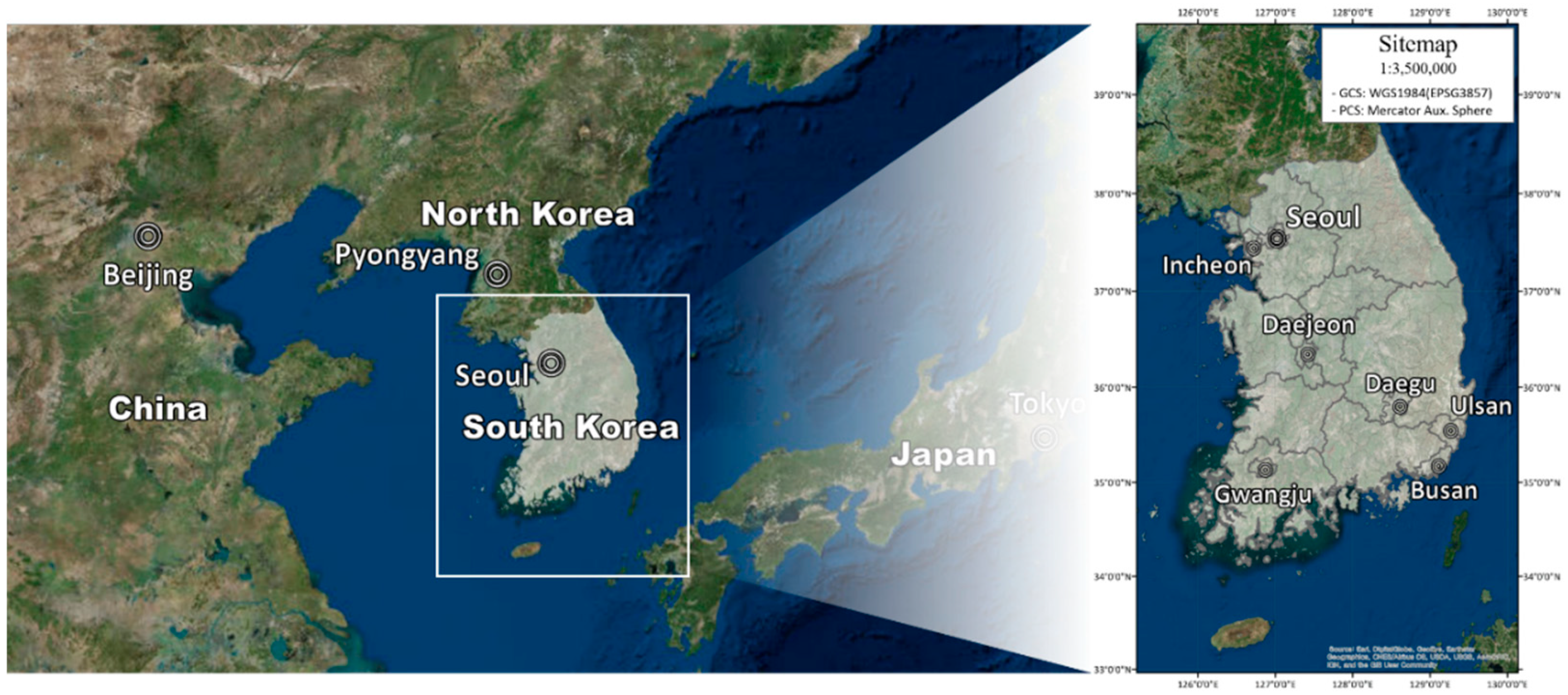
The spatial extent of this study is Korea (Figure 1). Korea underwent rapid urbanization along with great economic growth over the last 50 years, and, as a result, five major metropolitan areas were formed. To account for spatial uncertainties across the entire region, we set the extent of this study to include the Korean mainland, rather than focusing on a specific region, such as the Seoul metropolitan area.
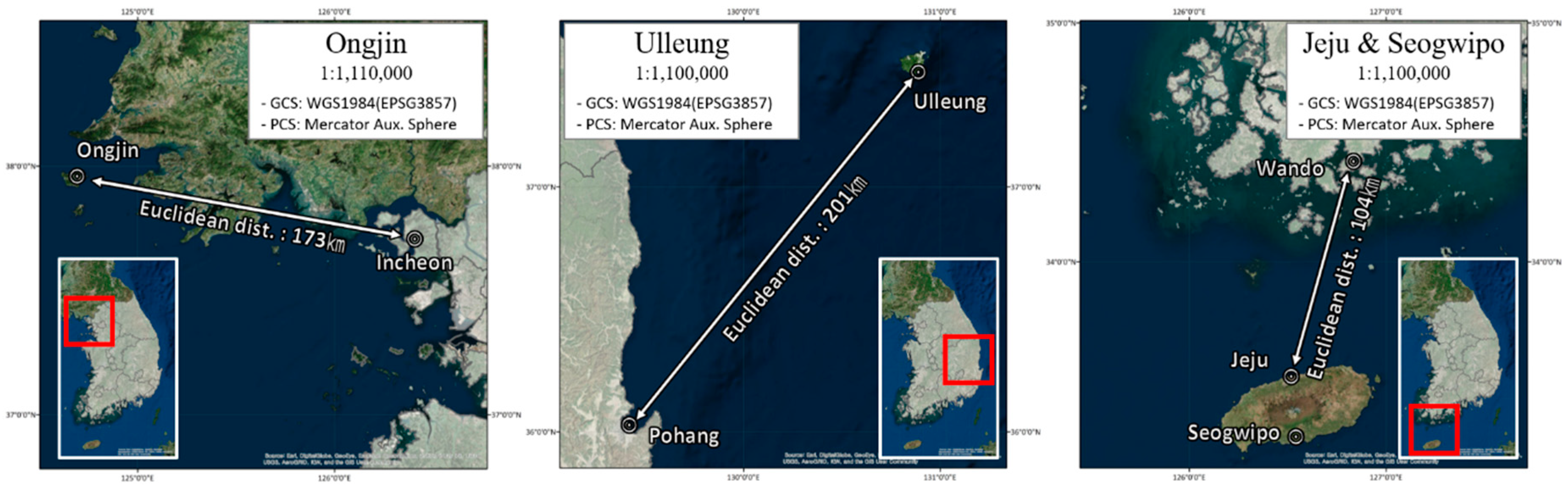
Korea has a four-level hierarchical administrative structure; in this study, the second-level administrative area, namely, Si (city)-Gun (county)-Gu (district) (SGG), is set as the spatial unit. An SGG corresponds to an administrative county in the United States. However, SGG presents fewer restrictions on the modifiable areal unit problem because the average area of SGGs (438 km2) is smaller than that of US counties (2,584 km2). In this study, the SGG is used as the unit of analysis. Korea consists of 229 SGGs, but four of them (Ongjin, Ulleung, Jeju, and Seogwipo) are excluded from this analysis because they are composed of islands located far from the mainland (Appendix Figure A1). In addition, these SGGs consistently emit marginal amounts of air pollutants. Therefore, 225 SGGs are used for our analysis.
2.2. Data and Variable
We consider four air pollutants, namely, NOX, SOX, PM10, and PM2.5, as response variables and use population size, area of commercial land use, area of industrial land use, area of park, road length, total land surface, and gross regional domestic product (GRDP) per person as covariates in this study. The number of observations for each variable is 225, and 2015 is set as the base year for all variables. In this section, we provide a detailed description of each variable.
Data on the four air pollutants by SGG are obtained from the National Air Pollutants Emission Service of the National Institute of Environmental Research. This annual dataset includes estimated amounts of air pollutants from 13 major pollutant sources by region (Appendix Table A1). Except for those on PM2.5, which were collected beginning 2011, data on the three other pollutants were collected from 1999 to 2015. However, analyzing the panel data is challenging because of discontinuities in emission estimates due to annual enhancement of emission factors and addition of new sources or removal of existing sources. Therefore, only the latest dataset (2015) is used for the analysis.
Another dataset on air pollutants is estimated not on the basis of pollutant sources but, rather, on the measurement instruments. Such data are not used in this study due to limitations associated with the control of external factors, including weather conditions. Several studies have found a strong relationship between the concentrations of air pollution and climatic variables, such as wind direction and speed [20,43,44,45,46,47]. In particular, Korea is heavily affected by pollutants from Northeast Asian regions due to its geographical characteristics and westerlies. Therefore, air pollutant data based on measurement instruments can contain air pollutants from both domestic and foreign sources, which can distort the true relationship between the country’s urban structures and air pollutant emissions. To avoid this problem, we use 1-year cross-sectional estimated emission data from domestic pollutant sources.
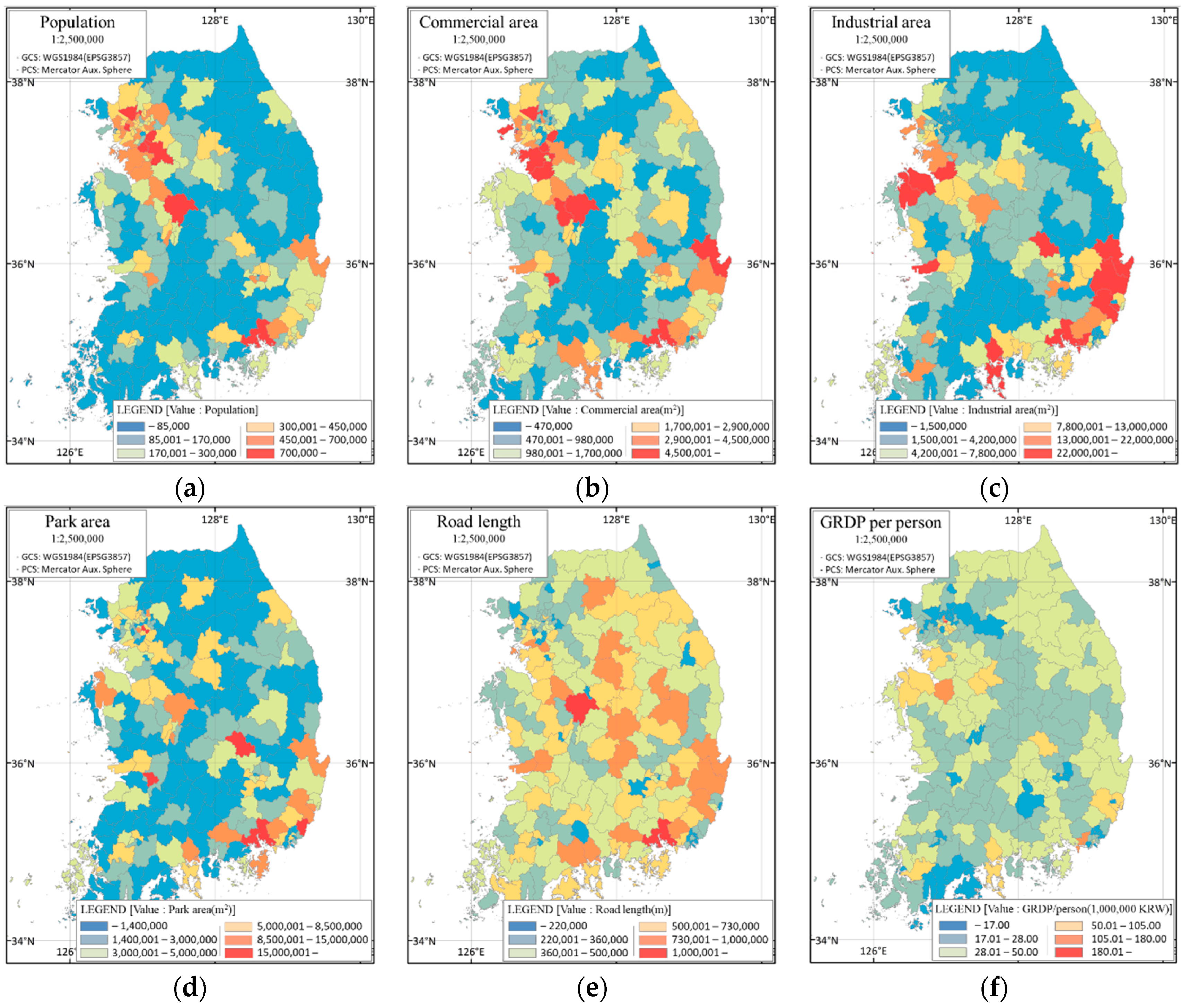
In this manuscript, we consider multiple covariates to account for complex urban structures. First, we include the population size of SGGs in the models. Population size has been used for scaling analysis to reveal diverse urban indicators [48,49,50,51]. The population can be used to determine the intensity of various socioeconomic activities causing complex urban structures. Second, we choose areas of commercial and industrial land use as covariates. Although the population can represent the area of residential land use, it cannot adequately cover commercial or industrial areas. For example, if SGGs near major metropolitan areas are bedroom towns, they must have a high proportion of residential area with a low proportion of commercial and industrial areas. By contrast, if SGGs are central business districts (CBDs), they must have a high proportion of commercial space and a low proportion of residential area due to the CBD hollowing-out phenomenon. Therefore, we use areas of commercial and industrial land use to account for the different regional characteristics of urban structures in each SGG. Third, we include the area of green spaces in SGGs in the models. In the context of environmental sustainability, the importance of green spaces to residents has been increasingly emphasized [31,32]. A potential variable for this approach is the area of a green zone defined by the National Land Planning and Utilization Act. However, this method is unsuitable because it includes areas of agricultural lands, such as farmland and production forest land, which are planted with crops focused on economic, rather than environmental, considerations. Hence, we use the area of parks defined as urban parks as a variable. Fourth, the length of all roads in SGGs regardless of pavement type is included in the models. The inclusion of road length in the analysis is reasonable because a considerable volume of air pollutants is directly emitted by the transportation sector [28]. Fifth, to control potential bias due to the different surfaces of each SGG, we include the total land area of each SGG in our models as in [37,38,39]. Finally, we include per capita real GRDP by SGG for 2015, the base year of which is 2010, to control the economic level on the relationship between urban structure and air pollutants. All urban structure variables are obtained from the Korean Statistical Information Service of Statistics Korea. The descriptive statistics and distributions of the original variables are summarized in Table 1 and Figure 2, respectively. Four air pollutants and seven covariates are transformed into a natural logarithm before descriptive and empirical analyses to improve normality [52,53,54].
The Korea Geographic Information Service (GIS) map used to present air pollutant emissions and local spatial autocorrelations is downloaded from the Statistical Geographic Information Service of Statistics Korea. All explanatory spatial data analyses are performed using ArcGIS 10.3 by ESRI.
2.3. Distributions of Air Pollutants
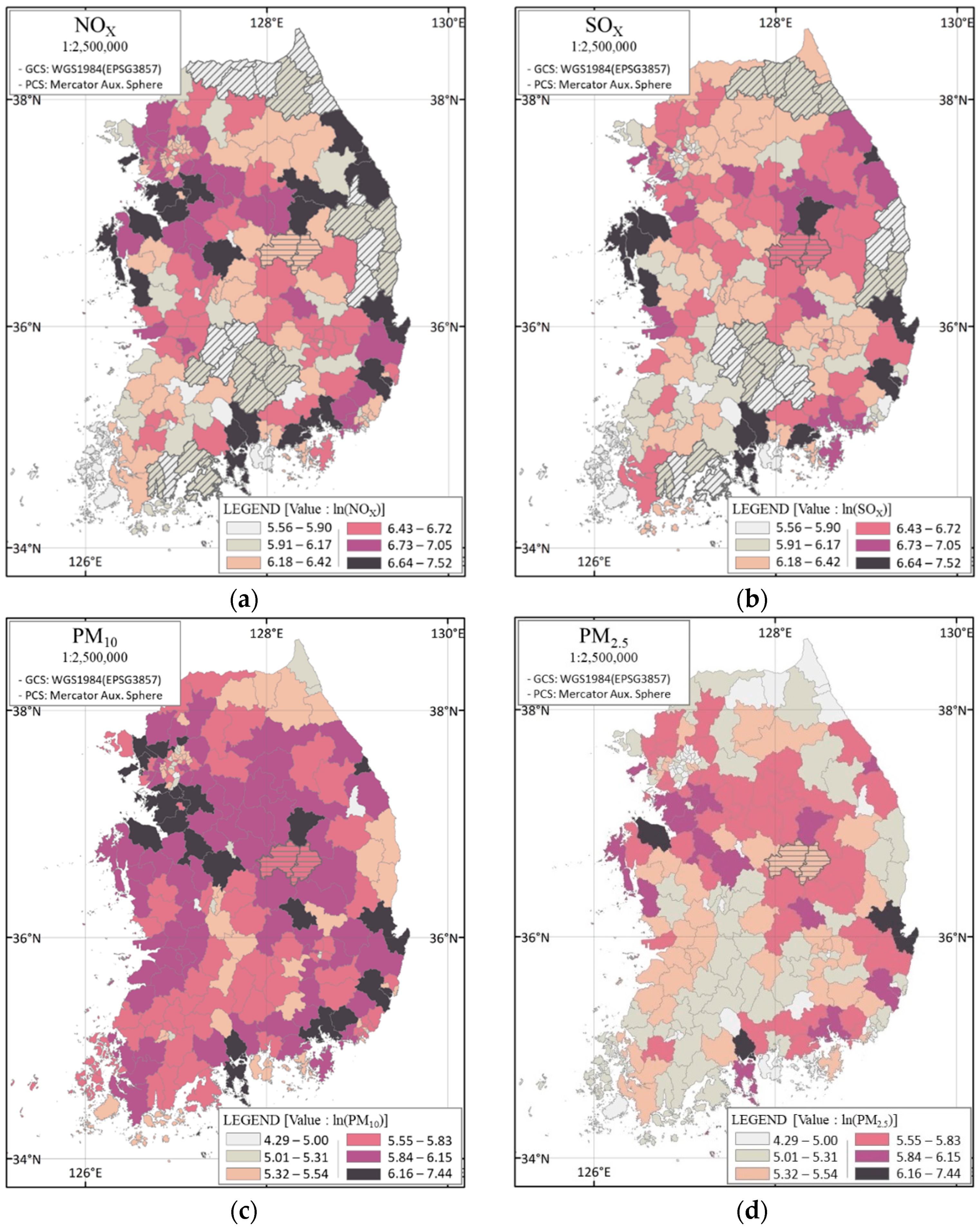
The distributions of the four air pollutants are illustrated in Figure 3. In terms of NOX and SOX, SGGs show a similar pattern of emission distribution. For example, areas marked by diagonal lines included in the lowest and second-lowest categories (e.g., southern coastal SGGs, southern inland SGGs, eastern coastal SGGs, and northeastern SGGs) emit relatively low amounts of pollutants (Figure 3a,b). By contrast, eastern coastal SGGs (37°–38° north latitude), which are positioned above the diagonal-line regions, southeastern SGGs, and midwest coastal SGGs emit high amounts of NOX and SOX. These SGGs possess manufacturing-oriented industrial complexes, thermoelectric power plants, and coal-fired power plants that are over 30 years old. PM10 emissions are generally higher than PM2.5 emissions, but some SGGs are included in the largest category of both types of particulate matter. Although overall patterns are similar among the four air pollutants, this finding does not mean that all individual SGGs have similar levels of emission of each pollutant. In other words, the amounts of pollutants emitted by each SGG may vary. For example, two SGGs (Mungyeong and Yecheon), which feature horizontal stripes in all pollutants, have relatively high emissions of SOX and PM10 (included in the top 50% categories) and low emissions of NOX and PM2.5 (included in the bottom 50% categories); by contrast, other SGGs show the opposite case. These results confirm the necessity of considering regional characteristics when analyzing air pollution.
In summary, we present three findings. (1) Although the four air pollutants are produced by different sources and mechanisms, the overall emissions of SGGs present similar patterns. (2) Some SGGs present different amounts of pollutant emissions due to regional differences in energy consumption and industrial structure. (3) Some adjacent SGGs that produce similar degrees of emissions form spatial clusters. On the basis of these findings, exploratory spatial data analyses are conducted, and spatial linear models are fitted for further analysis.
3. Methodology
3.1. Exploratory Spatial Data Analysis
Statistical inference in the presence of spatial autocorrelation is challenging because dependencies among nearby SGGs can lead to unreliable parameter estimates. For example, Dong and Liang [55] noted the presence of global and local spatial dependencies in emissions of various pollutants in China, and Réquia et al. [56] discovered the existence of clusters in various types of pollutant emissions. In this study, spatial autocorrelations of emissions can arise in urban structures, such as in industrial complexes or power plants where emission sources are usually agglomerated due to economic reasons. To determine if spatial autocorrelation issues exist in our study, we use Global Moran’s I, a popular nonparametric statistics of spatial autocorrelation [57]. Moran’s I can detect spatial dependence by calculating the correlation among nearby regions. If Moran’s I is statistically significant, spatial linear regression models should be fitted to account for such dependence among the data.
We calculate Global Moran’s I to check whether or not global spatial autocorrelations occur. Although Global Moran’s I can be a proxy for global spatial autocorrelation, it does not represent local clusters. Local deviations from a global pattern of spatial autocorrelation can occur even if the entire study area has a significant spatial autocorrelation. Thus, we also apply Local Moran’s I, which decomposes Global Moran’s I, to identify local clusters of each pollutant [58]. A positive value of Local Moran’s I means that the emission values for an SGG are similar to those of adjacent SGGs. Then, this SGG becomes part of a high-high or low-low cluster. By contrast, a negative value of Local Moran’s I represents dissimilar emission values among nearby regions. Then, this SGG is part of a high-low or low-high outlier. The details for the spatial weight matrix for Moran’s I are provided in Section 3.2.
3.2. Spatial Linear Regression Model
In the presence of spatial autocorrelations, adding a set of spatially correlated random effects to the linear predictor is the most common approach to account for such dependencies. These random effects are typically modeled with a conditional autoregressive (CAR) prior [59], which can incorporate spatial dependence among neighboring areal units. Lee [60] compared several variants of CAR models and identified the model proposed by Leroux et al. [61] as the most general and practical approach; therefore, we use this model in our analysis. The hierarchical structure of spatial linear models renders the Bayesian approach convenient to use. For example, Bayesian spatial regression models have been widely used to analyze the relationship between air pollution and health in Scotland [62] and estimate the effects of air pollution on respiratory hospital admissions in London [63]. Liu et al. [64] predicted air quality in Xiamen, China, by using a Bayesian hierarchical model.
In this context, Bayesian spatial linear regression models are fitted to examine the relationship between the covariates and response variables, namely, NOX, SOX, PM10, and PM2.5 models. We have n = 225 number of observations across the spatial domain and p = 7 number of predictors. We let Y be a 225 × 1 response variable vector and X be a 225 × 7 matrix of values of covariates. We note that Y is log-transformed air pollutants and X is log-transformed urban structure and control variables. Our models can be written as follows:
where β is a regression coefficient and is a spatial random effect. is modeled by a CAR [59,61] prior distribution to incorporate spatial dependence among observations as follows:
where is a spatial autocorrelation parameter and is a variance parameter. The covariance structure of is determined by selecting spatial weight matrix W that summarizes the spatial associations among observations. The priors for our parameters of interest are:
We infer the model parameters via a Bayesian approach by using a Markov chain Monte Carlo (MCMC) algorithm. The code for statistical analysis is implemented by using the CARBayes [65] package in R [66].
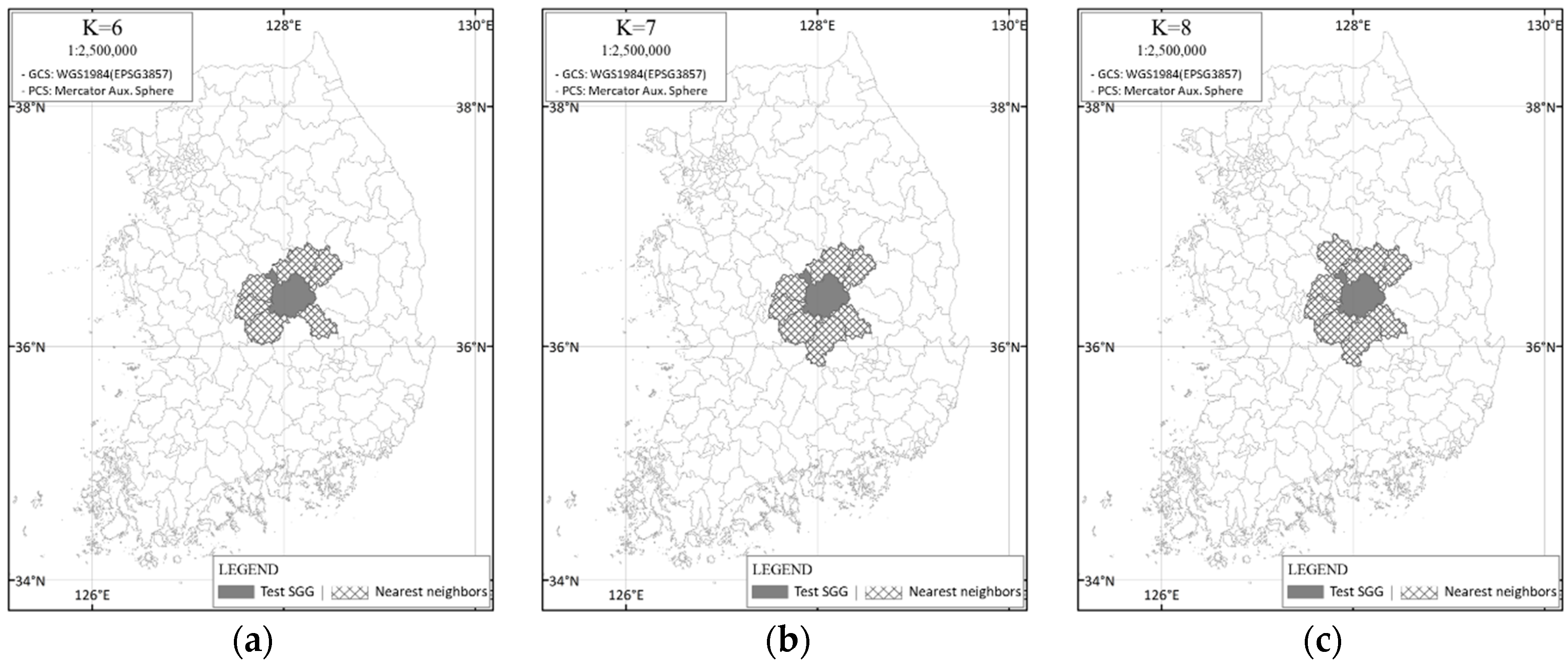
For spatial weight matrix W, we use k-nearest neighbor weights based on the Euclidean distance of the centroid of areal units. An SGG is unlikely to have more than eight neighbors; therefore, we set the range of k from 3 to 8. We use the Bayesian information criterion (BIC) to select k for each model. The implementation proceeds as follows. (1) We fit spatial regression models for each of the response variables (NOX, SOX, PM10, and PM2.5) with different k values. (2) BIC values are calculated, and a small BIC indicates a good model. We then select models with the smallest BIC for each of the response variables. (3) To validate our analysis, we calculate the Global Moran’s I for each model’s residuals. When the Global Moran’s I value is significantly small, the models successfully account for spatial autocorrelation.
4. Results
The Global Moran’s I values for air pollutants are summarized in Table 2. All values are significantly positive, which means that pollutants are clustered together. In particular, the Global Moran’s I value for PM2.5 is higher than that for other pollutants. Hence, PM2.5 is more clustered than the other pollutants are. Our result reveals the existence of spatial autocorrelation in emissions and thus provides theoretical justifications for using spatial linear regression models.
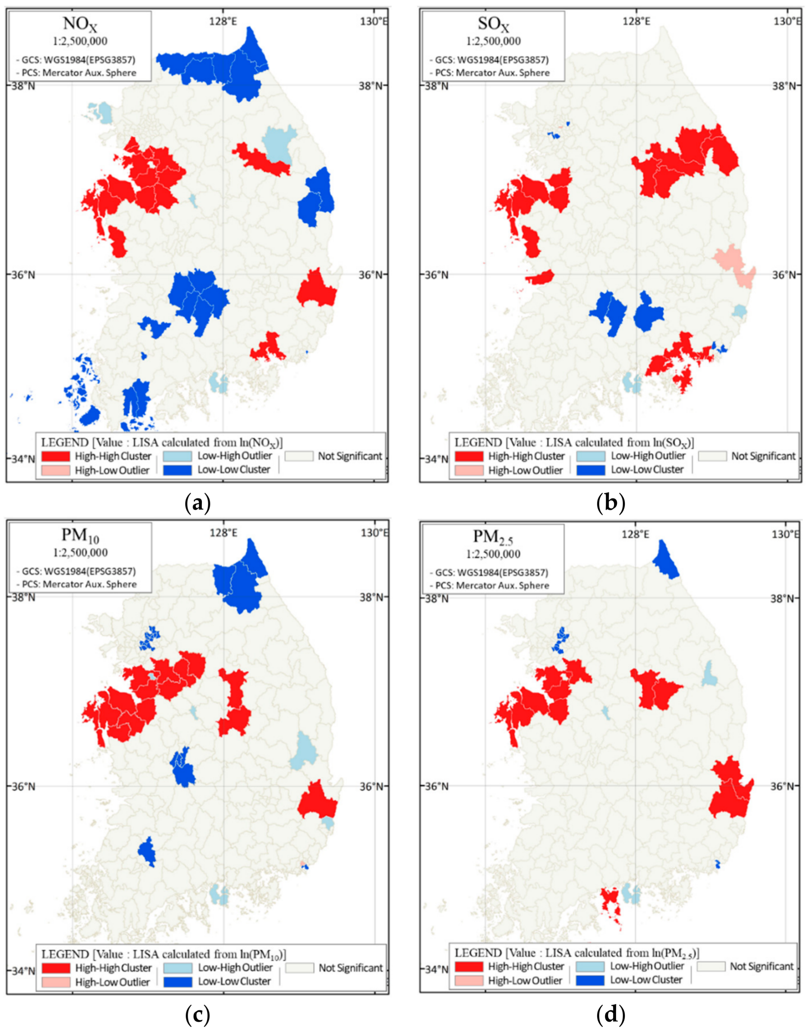
We also examine the local clusters and outliers of each pollutant (Figure 4). Each air pollutant has a different local spatial pattern. For example, most of the high-high clusters of NOX are located in western coastal areas, and many of the high-high clusters of SOX are at 37° north latitude, especially in either eastern or western coastal regions. With regard to two types of particulate matter, most of the high-high clusters of PM10 and PM2.5 are at 37° north latitude or in eastern coastal areas at 36° north latitude. In terms of low-low clusters, NOX have more clusters than other pollutants do, and the clusters are distributed all over the study area. Meanwhile, SOX and PM2.5 have distinctly few low-low clusters indicating that an SGG with low emission of either SOX or PM2.5 does not cluster together.
Several implications for further analysis are deduced on the basis of the spatial pattern of clusters. (1) The distributions of statistically calculated clusters are in discord with those of descriptive clusters in Figure 3 to some degree. For example, not all diagonal-line areas of NOX and SOX indicate low emissions form low-low clusters. (2) Several SGGs are included in the high-high clusters of four pollutants, indicating that common urban characteristics can occur among these SGGs. In other words, several urban structure factors can influence the emissions regardless of air pollutant type. For example, several western coastal SGGs where national industrial complexes are located are included in each high-high cluster of four pollutants. (3) By contrast, the different distribution of clusters indicates that the relationship might differ by air pollutants. The degree of influence may vary by pollutant even if urban structure variables affect emissions. The results of Global and Local Moran’s I suggest potential spatial dependencies of air pollutants. Therefore, we use a spatial regression model as a rigorous approach to investigate the relationship between urban structures and each air pollutant.
We select k for each spatial regression model based on the BIC values summarized in Table 3. On the basis of the results in Table 3, we choose k = 8 for the NOX model, k = 7 for the SOX model, and k = 6 for the PM10 and PM2.5 models. Figure 5 shows the extent of spatial dependencies among SGGs for different k values.
The estimated regression coefficients for each model are summarized in Table 4. When the response variables are NOX, PM10, and PM2.5, coefficients for population, industrial area, total land surface, and GRDP per person are positively significant. When the response variable is SOX, commercial area, industrial area, and GRDP per person are significant, and the coefficients are positively estimated. The coefficients for industrial area and GRDP per person are positively significant across all models.
In general, significant covariates show positive values, and the magnitude of the values is smaller than that of the one-to-one correspondence in the relationships. In other words, a 1% increase in urban structure variables results in increments in emissions of air pollutants by less than 1%. These results show that the negative effects of urbanization can be mitigated in the concept of efficiency.
First, when the population increases by 1%, the emissions of NOX, PM10, and PM2.5 increase by 0.565%, 0.456%, and 0.379%, respectively. These positive effects are reasonable because population size determines the size of the residential area and the degree of socioeconomic activities in the regions. Meanwhile, an increase in the area of commercial land use is significant only on SOX (0.529%). Given that the commercial area considered here includes traditional and distribution commercial districts, the positive influence of commercial area on the emission of SOX is sensible. Increments in the area of industrial land use commonly show increments in emissions. An industrial area primarily is filled with secondary industries that are one of the primary sources of air pollutants, especially SOX. However, a park area, which is assumed to have negative impacts on emissions, is not significant in all models. This is because although the park area exists in the region, we cannot determine the amounts, kinds, and spatial patterns of plants within the park that are directly related to the reduction of air pollutants. The road length variable is not statistically significant to the emissions of all air pollutants, which may seem counterintuitive, because a potential confounding issue exists in this variable. For example, a two-lane back road and an eight-lane main road can have the same length. However, the emissions from the two roads are completely different because of the difference in traffic volumes, road widths, and average vehicle speeds. Considering this additional information for each road is challenging in practice. The total land surface is positively significant to the emissions of air pollutants, except for SOX. In particular, the emissions of the two types of particulate matter increase more than the emission of NOX. This result indicates that large areas usually have many particulate matter pollutant sources. Moreover, increases in GRDP per person have positively significant effects on pollutant emissions, but their degrees are relatively small. We conclude that the impact of regional economic level on air pollution is lower than that of the urban structure in Korea.
Table 5 shows the Global Moran’s I values for each model’s residuals. The absolute values of all pollutants, except for the SOX model, are insignificant. Thus, the Bayesian models (NOX, PM10, and PM2.5) effectively account for the spatial dependencies. Although the SOX model’s Global Moran’s I value is significant, the value decreases from 0.191 to 0.103, which means the model accounts for spatial autocorrelation.
5. Discussion and Conclusions
Korea has pushed ahead with urbanization through government-initiated planning. Hence, its urban structures have become complicated. At the same time, air pollution as a serious environmental issue has recently elicited attention in Korea. Spatial models for underlying mechanisms are critical for estimating emissions of air pollutants from urban structures and for accounting for regional characteristics. Against this background, we study the spatial relationship between urban structures and emissions of air pollutants via exploratory data analyses and Bayesian spatial regression models. Our approach provides a general framework for analyzing spatial relationships between different air pollutants and urban structure covariates. The results show a smaller increase than the direct proportion in the emissions of air pollutants with increasing urban structure variables. This finding is crucial because it suggests that urbanization progress does not result in a one-to-one negative influence on air pollution. Previous studies have focused on investigating the relationship between few urban structure variables and the emission of a particular air pollutant. By contrast, we use multiple regression models to address the uncertainty in the underlying mechanisms. Population size is significant, except in the SOX model, and it conforms to the results of other studies [33,37]. Furthermore, population coefficients are estimated to be less than one, which indicates that the innovation effect occurs in urban areas in the context of scaling analysis [48,49,50,51]. The positively significant regression coefficients for commercial and industrial areas in the SOX model are similar to the results of Cárdenas Rodríguez et al. [38].
The insignificant park area in all the models supports the study of McCarty and Kaza [37]. However, the spatial pattern of the forest variable considered in their research has a positive influence on the atmospheric environment. The traffic-related variable, which was assumed to be the major cause of low air quality in the study of Hussein at al. [28], is not significant in our study. This result can be due to the confounding of the road length variable as we pointed out in Section 4. Furthermore, a variable related to local economic levels can be used to identify unique relationships between air pollution and economic growth in Korea. On the basis of the positive coefficients for GRDP per person, we find that economic growth negatively affects air conditions in Korea. This finding is in contrast with the results of McCarty [37] and Cárdenas Rodríguez et al. [38], who found that economic level covariates show negative relations with air pollutant variables in the United States and Europe, respectively. Our findings align with the results of Kim and Oh [67], who found positive relationships between economic growth and air pollution in Korea. This fact demonstrates the importance of implementing Korea-specific air-related policies.
Policies for urban development should be planned according to the degree of urban structure and the pollutant level by region. In this process, scenario planning can be introduced to achieve sustainable development by considering ecosystem functions [68,69]. One of the applicable scenarios is that most SGGs are in the urbanization terminal stage. This scenario indicates that many regions have a complex urban structure with a large population that is difficult to change. In this situation, rapidly changing existing areas that are closely related to the emission of air pollutants to other uses is difficult because of numerous economic and social limitations. Hence, the government should recommend a means of maintaining current uses and reducing emissions without manipulating the existing ecosystem. The approach is linked to a smart city, which is a concept for the future in Korea. The smart city plan aims to respond to urban environmental problems, including air pollution, and ultimately block pollution in advance by introducing new technologies in the existing urban structure [70,71]. Thus, the government can reduce air pollution without radical urban transformations.
Furthermore, regional policies should be applied differently depending on the pollutant level because emissions by pollutants vary from region to region. Cárdenas Rodríguez et al. [34] found that positively significant correlations occur between nitrogen dioxide and PM10 and between sulfur dioxide and PM10. Thus, a region with a high level of a specific pollutant may also have a high level of other air pollutants. However, regional differences remain in air pollution. The local government should examine and understand the condition of regional air pollution and apply air pollution reduction policies in consideration of its urban structure characteristics. An air pollution policy, the “Clean Air Conservation Act,” suggests local government action toward regional pollution, but the policy still targets high administrative units. Furthermore, if a region and its neighboring areas have a similar level of a specific air pollutant, then a macro approach that considers these areas’ structures together is required.
In this study, we use multiple urban structure covariates by considering composition factors, such as size and area, in investigating the underlying mechanisms. We note that the configuration of the urban structures, which can affect the emission of air pollutants as well, must be considered. For example, the widely distributed industrial complex and agglomerated industrial complex may have a different influence on emissions even if both complexes have the same area. The remote-sensing method might provide raster data for configuration information. However, in the interest of clear model interpretation and the limited availability of configuration data on urban structures, our urban structure covariates appear to be a good choice. The other open question is how to conceptualize the green area and transportation factors in the urban area. We use park area and road length as practical proxies, but they have potential confounding issues as we pointed out in the previous sections. However, finding appropriate proxies poses significant challenges in practice.
In summary, we investigate the relationship between urban structures and emissions of air pollutants in Korea. The descriptive distribution of emissions of four air pollutants presents the degree of local emission by pollutants. SGGs with agglomerated industry complexes or large populations usually emit large amounts of air pollutants. We use Bayesian spatial linear regression models to account for existing spatial dependencies and to study the underlying mechanisms. We utilize population size, commercial area, industrial area, park area, road length, total land surface, and GRDP per person as spatial covariates. The results provide a theoretical implication for countries that are at the end of the acceleration stage or at the beginning of the terminal stage of urbanization. The models indicate that urbanization does not result in a one-to-one negative influence on air pollution. However, the government should consider sustainable development because a positive relationship exists between urbanization and air pollutant emissions. In this context, the smart city concept and scenario planning can be considered in the policy making process to achieve a sustainable environment.
Author Contributions
M.C.J. conceived the design of this study, performed an explanatory data analysis, and wrote the manuscript. J.P. conducted the statistical analysis and wrote the method section. S.K. conceived the design of this study and performed the visualization of GIS maps. M.C.J., J.P., and S.K. participated in revising the manuscript.
Funding
This research received no external funding.
Acknowledgments
The authors are grateful to the anonymous reviewers and Karen Dyson for providing constructive feedback on the manuscript. This research is based on the result of “Seoul Research Competition 2017”, which is the outstanding paper award.
Conflicts of Interest
The authors declare no conflict of interest.
Appendix A
Figure A1.
Locations of four excluded SGGs.


Table A1.
Classification of pollutant sources.
| Pollutant Source | |
|---|---|
| 1 | Combustion in energy and transformation industry |
| 2 | Non-industrial combustion plants |
| 3 | Combustion in manufacturing industry |
| 4 | Production processes |
| 5 | Extraction and distribution of fossil fuels |
| 6 | Solvent and other product use |
| 7 | Road transport |
| 8 | Other mobile sources and machinery |
| 9 | Waste treatment and disposal |
| 10 | Agriculture |
| 11 | Other sources and skins |
| 12 | Fugitive dust |
| 13 | Biomass combustion |
References
- Anas, A.; Arnott, R.; Small, K.A. Urban Spatial Structure. J. Econ. Lit. 1998, 36, 1426–1464. [Google Scholar]
- Fujita, M.; Ogawa, H. Multiple equilibria and structural transition of non-monocentric urban configurations. Reg. Sci. Urban Econ. 1982, 12, 161–196. [Google Scholar] [CrossRef]
- Garcia-López, M.-À.; Muñiz, I. Urban spatial structure, agglomeration economies, and economic growth in Barcelona: An intra-metropolitan perspective. Pap. Reg. Sci. 2013, 92, 515–534. [Google Scholar] [CrossRef]
- Rosenthal, S.S.; Strange, W.C. Chapter 49—Evidence on the Nature and Sources of Agglomeration Economies. In Handbook of Regional and Urban Economics; Henderson, J.V., Thisse, J.-F., Eds.; Cities and Geography; Elsevier: Amsterdam, The Netherlands, 2004; Volume 4, pp. 2119–2171. [Google Scholar]
- Pan, H.; Deal, B.; Chen, Y.; Hewings, G. A Reassessment of urban structure and land-use patterns: Distance to CBD or network-based—Evidence from Chicago. Reg. Sci. Urban Econ. 2018, 70, 215–228. [Google Scholar] [CrossRef]
- Marrocu, E.; Paci, R.; Usai, S. Productivity Growth in the Old and New Europe: The Role of Agglomeration Externalities. J. Reg. Sci. 2013, 53, 418–442. [Google Scholar] [CrossRef]
- Habitat, U.N. Urbanization and Development Emerging Futures. Available online: https://www.unhabitat.org/wp-content/uploads/2014/03/WCR-%20Full-Report-2016.pdf (accessed on 17 January 2019).
- Borrego, C.; Martins, H.; Tchepel, O.; Salmim, L.; Monteiro, A.; Miranda, A.I. How urban structure can affect city sustainability from an air quality perspective. Environ. Model. Softw. 2006, 21, 461–467. [Google Scholar] [CrossRef]
- Chan, C.K.; Yao, X. Air pollution in mega cities in China. Atmos. Environ. 2008, 42, 1–42. [Google Scholar] [CrossRef]
- Krishna, I.V.M.; Manickam, V.; Shah, A.; Davergave, N. Environmental Management: Science and Engineering for Industry; Butterworth-Heinemann: Oxford, UK, 2017; ISBN 978-0-12-811990-7. [Google Scholar]
- Marquez, L.O.; Smith, N.C. A framework for linking urban form and air quality. Environ. Model. Softw. 1999, 14, 541–548. [Google Scholar] [CrossRef]
- Balkytė, A.; Tvaronavičienė, M. Perception of Competitiveness in the Context of Sustainable Development: Facets of “Sustainable Competitiveness”. J. Bus. Econ. Manag. 2010, 11, 341–365. [Google Scholar] [CrossRef]
- Briggs, D.; Abellan, J.J.; Fecht, D. Environmental inequity in England: Small area associations between socio-economic status and environmental pollution. Soc. Sci. Med. 2008, 67, 1612–1629. [Google Scholar] [CrossRef]
- Guarnieri, M.; Balmes, J.R. Outdoor air pollution and asthma. Lancet 2014, 383, 1581–1592. [Google Scholar] [CrossRef] [Green Version]
- Janssen, N.A.H.; Hoek, G.; Fischer, P.H.; Wijga, A.H.; Koppelman, G.; de Jongste, J.J.; Brunekreef, B.; Gehring, U. Joint Association of Long-term Exposure to Both O3 and NO2 with Children’s Respiratory Health. Epidemiology 2017, 28, e7–e9. [Google Scholar] [CrossRef]
- Lelieveld, J.; Evans, J.S.; Fnais, M.; Giannadaki, D.; Pozzer, A. The contribution of outdoor air pollution sources to premature mortality on a global scale. Nature 2015, 525, 367–371. [Google Scholar] [CrossRef] [PubMed]
- Medina, S.; Plasencia, A.; Ballester, F.; Mücke, H.G.; Schwartz, J. Apheis: Public health impact of PM10 in 19 European cities. J. Epidemiol. Community Health 2004, 58, 831–836. [Google Scholar] [CrossRef] [PubMed]
- Pope, C.A., III; Dockery, D.W. Health Effects of Fine Particulate Air Pollution: Lines that Connect. J. Air Waste Manag. Assoc. 2006, 56, 709–742. [Google Scholar] [Green Version]
- Seo, S.; Kim, D.; Min, S.; Paul, C.; Yoo, Y.; Choung, J.T. GIS-based Association Between PM10 and Allergic Diseases in Seoul: Implications for Health and Environmental Policy. Allergy Asthma Immunol. Res. 2016, 8, 32–40. [Google Scholar] [CrossRef]
- Jang, Y.-K. Current Status and Problems of Particulate Matter Pollution. J. Environ. Stud. 2016, 58, 4–13. [Google Scholar]
- Lee, J.H.; Kim, Y.M.; Kim, Y. Spatial panel analysis for PM2.5 concentrations in Korea. J. Korean Data Inf. Sci. Soc. 2017, 28, 473–481. [Google Scholar]
- Schneider, P.; Lahoz, W.A.; van der A, R. Recent satellite-based trends of tropospheric nitrogen dioxide over large urban agglomerations worldwide. Atmos. Chem. Phys. 2015, 15, 1205–1220. [Google Scholar] [CrossRef] [Green Version]
- van der Wal, J.T.; Janssen, L.H.J.M. Analysis of spatial and temporal variations of PM 10 concentrations in the Netherlands using Kalman filtering. Atmos. Environ. 2000, 34, 3675–3687. [Google Scholar] [CrossRef]
- Wang, Y.; Zhang, Q.Q.; He, K.; Zhang, Q.; Chai, L. Sulfate-nitrate-ammonium aerosols over China: Response to 2000–2015 emission changes of sulfur dioxide, nitrogen oxides, and ammonia. Atmos. Chem. Phys. 2013, 13, 2635–2652. [Google Scholar] [CrossRef]
- van Donkelaar, A.; Martin, R.V.; Brauer, M.; Kahn, R.; Levy, R.; Verduzco, C.; Villeneuve, P.J. Global Estimates of Ambient Fine Particulate Matter Concentrations from Satellite-Based Aerosol Optical Depth: Development and Application. Environ. Health Perspect. 2010, 118, 847–855. [Google Scholar] [CrossRef] [PubMed] [Green Version]
- Chai, F.; Gao, J.; Chen, Z.; Wang, S.; Zhang, Y.; Zhang, J.; Zhang, H.; Yun, Y.; Ren, C. Spatial and temporal variation of particulate matter and gaseous pollutants in 26 cities in China. J. Environ. Sci. 2014, 26, 75–82. [Google Scholar] [CrossRef]
- Xu, L.; Batterman, S.; Chen, F.; Li, J.; Zhong, X.; Feng, Y.; Rao, Q.; Chen, F. Spatiotemporal characteristics of PM2.5 and PM10 at urban and corresponding background sites in 23 cities in China. Sci. Total Environ. 2017, 599–600, 2074–2084. [Google Scholar] [CrossRef] [PubMed]
- Hussein, T.; Hämeri, K.; Aalto, P.P.; Paatero, P.; Kulmala, M. Modal structure and spatial–temporal variations of urban and suburban aerosols in Helsinki—Finland. Atmos. Environ. 2005, 39, 1655–1668. [Google Scholar] [CrossRef]
- Oh, K.-S.; Chung, H.-B. The Influence of Urban Development Density on Air Pollution. J. Korea Plan. Assoc. 2007, 42, 197–210. [Google Scholar]
- Sánchez-Rodas, D.; Sánchez de la Campa, A.M.; de la Rosa, J.D.; Oliveira, V.; Gómez-Ariza, J.L.; Querol, X.; Alastuey, A. Arsenic speciation of atmospheric particulate matter (PM10) in an industrialised urban site in southwestern Spain. Chemosphere 2007, 66, 1485–1493. [Google Scholar] [CrossRef]
- Freiman, M.T.; Hirshel, N.; Broday, D.M. Urban-scale variability of ambient particulate matter attributes. Atmos. Environ. 2006, 40, 5670–5684. [Google Scholar] [CrossRef]
- Fantozzi, F.; Monaci, F.; Blanusa, T.; Bargagli, R. Spatio-temporal variations of ozone and nitrogen dioxide concentrations under urban trees and in a nearby open area. Urban Clim. 2015, 12, 119–127. [Google Scholar] [CrossRef]
- Cho, H.-S.; Choi, M.J. Effects of Compact Urban Development on Air Pollution: Empirical Evidence from Korea. Sustainability 2014, 6, 5968–5982. [Google Scholar] [CrossRef] [Green Version]
- Stone, B. Urban sprawl and air quality in large US cities. J. Environ. Manag. 2008, 86, 688–698. [Google Scholar] [CrossRef] [PubMed]
- Bereitschaft, B.; Debbage, K. Urban Form, Air Pollution, and CO2 Emissions in Large U.S. Metropolitan Areas. Prof. Geogr. 2013, 65, 612–635. [Google Scholar] [CrossRef]
- Schweitzer, L.; Zhou, J. Neighborhood Air Quality, Respiratory Health, and Vulnerable Populations in Compact and Sprawled Regions. J. Am. Plann. Assoc. 2010, 76, 363–371. [Google Scholar] [CrossRef]
- McCarty, J.; Kaza, N. Urban form and air quality in the United States. Landsc. Urban Plan. 2015, 139, 168–179. [Google Scholar] [CrossRef]
- Cárdenas Rodríguez, M.; Dupont-Courtade, L.; Oueslati, W. Air pollution and urban structure linkages: Evidence from European cities. Renew. Sustain. Energy Rev. 2016, 53, 1–9. [Google Scholar] [CrossRef]
- Clark, L.P.; Millet, D.B.; Marshall, J.D. Air Quality and Urban Form in U.S. Urban Areas: Evidence from Regulatory Monitors. Environ. Sci. Technol. 2011, 45, 7028–7035. [Google Scholar] [CrossRef] [PubMed]
- Gutenberg, S. Demystifying the Air Quality Health Index. Can. Pharm. J. Rev. Pharm. Can. 2014, 147, 332–334. [Google Scholar] [CrossRef] [PubMed] [Green Version]
- Gschwandtner, G.; Gschwandtner, K.; Eldridge, K.; Mann, C.; Mobley, D. Historic Emissions of Sulfur and Nitrogen Oxides in the United States from 1900 to 1980. J. Air Pollut. Control Assoc. 1986, 36, 139–149. [Google Scholar] [CrossRef] [Green Version]
- Suh, H.H.; Bahadori, T.; Vallarino, J.; Spengler, J.D. Criteria air pollutants and toxic air pollutants. Environ. Health Perspect. 2000, 108, 625–633. [Google Scholar]
- Harrison, R.M.; Deacon, A.R.; Jones, M.R.; Appleby, R.S. Sources and processes affecting concentrations of PM10 and PM2.5 particulate matter in Birmingham (U.K.). Atmos. Environ. 1997, 31, 4103–4117. [Google Scholar] [CrossRef]
- Liu, Z.; Hu, B.; Wang, L.; Wu, F.; Gao, W.; Wang, Y. Seasonal and diurnal variation in particulate matter (PM10 and PM2.5) at an urban site of Beijing: Analyses from a 9-year study. Environ. Sci. Pollut. Res. 2015, 22, 627–642. [Google Scholar] [CrossRef] [PubMed]
- Noble, C.A.; Mukerjee, S.; Gonzales, M.; Rodes, C.E.; Lawless, P.A.; Natarajan, S.; Myers, E.A.; Norris, G.A.; Smith, L.; Özkaynak, H.; et al. Continuous measurement of fine and ultrafine particulate matter, criteria pollutants and meteorological conditions in urban El Paso, Texas. Atmos. Environ. 2003, 37, 827–840. [Google Scholar] [CrossRef]
- Park, S.; Shin, H. Analysis of the Factors Influencing PM2.5 in Korea: Focusing on Seasonal Factors. J. Environ. Policy Adm. 2017, 25, 227–248. [Google Scholar] [CrossRef]
- Slini, T.; Kaprara, A.; Karatzas, K.; Moussiopoulos, N. PM10 forecasting for Thessaloniki, Greece. Environ. Model. Softw. 2006, 21, 559–565. [Google Scholar] [CrossRef]
- Bettencourt, L.M.A.; Lobo, J.; Helbing, D.; Kühnert, C.; West, G.B. Growth, innovation, scaling, and the pace of life in cities. Proc. Natl. Acad. Sci. USA 2007, 104, 7301–7306. [Google Scholar] [CrossRef] [Green Version]
- Bettencourt, L.M.A.; Lobo, J.; Strumsky, D.; West, G.B. Urban Scaling and Its Deviations: Revealing the Structure of Wealth, Innovation and Crime across Cities. PLoS ONE 2010, 5, e13541. [Google Scholar] [CrossRef] [PubMed]
- Bettencourt, L.M.A. The Origins of Scaling in Cities. Science 2013, 340, 1438–1441. [Google Scholar] [CrossRef]
- Fragkias, M.; Lobo, J.; Strumsky, D.; Seto, K.C. Does Size Matter? Scaling of CO2 Emissions and U.S. Urban Areas. PLoS ONE 2013, 8, e64727. [Google Scholar] [CrossRef]
- Gilbert, N.L.; Goldberg, M.S.; Beckerman, B.; Brook, J.R.; Jerrett, M. Assessing spatial variability of ambient nitrogen dioxide in Montreal, Canada, with a land-use regression model. J. Air Waste Manag. Assoc. 2005, 55, 1059–1063. [Google Scholar] [CrossRef]
- Henderson, S.B.; Beckerman, B.; Jerrett, M.; Brauer, M. Application of land use regression to estimate long-term concentrations of traffic-related nitrogen oxides and fine particulate matter. Environ. Sci. Technol. 2007, 41, 2422–2428. [Google Scholar] [CrossRef]
- Ross, Z.; Jerrett, M.; Ito, K.; Tempalski, B.; Thurston, G.D. A land use regression for predicting fine particulate matter concentrations in the New York City region. Atmos. Environ. 2007, 41, 2255–2269. [Google Scholar] [CrossRef]
- Dong, L.; Liang, H. Spatial analysis on China’s regional air pollutants and CO2 emissions: Emission pattern and regional disparity. Atmos. Environ. 2014, 92, 280–291. [Google Scholar] [CrossRef]
- Réquia, W.J.; Koutrakis, P.; Roig, H.L. Spatial distribution of vehicle emission inventories in the Federal District, Brazil. Atmos. Environ. 2015, 112, 32–39. [Google Scholar] [CrossRef]
- Moran, P.A.P. Notes on Continuous Stochastic Phenomena. Biometrika 1950, 37, 17–23. [Google Scholar] [CrossRef] [PubMed]
- Anselin, L. Local Indicators of Spatial Association—LISA. Geogr. Anal. 1995, 27, 93–115. [Google Scholar] [CrossRef]
- Besag, J.; York, J.; Mollié, A. A Bayesian image restoration with two applications in spatial statistics. Ann. Inst. Stat. Math. 1991, 43, 1–59. [Google Scholar] [CrossRef]
- Lee, D. A comparison of conditional autoregressive models used in Bayesian disease mapping. Spat. Spatio-Temporal Epidemiol. 2011, 2, 79–89. [Google Scholar] [CrossRef]
- Leroux, B.G.; Lei, X.; Breslow, N. Estimation of disease rates in small areas: A new mixed model for spatial dependence. In Statistical Models in Epidemiology, the Environment, and Clinical Trials; Springer: New York, NY, USA, 2000; pp. 179–191. [Google Scholar]
- Lee, D.; Ferguson, C.; Mitchell, R. Air pollution and health in Scotland: A multicity study. Biostatistics 2009, 10, 409–423. [Google Scholar] [CrossRef]
- Rushworth, A.; Lee, D.; Mitchell, R. A spatio-temporal model for estimating the long-term effects of air pollution on respiratory hospital admissions in Greater London. Spat. Spatio-Temporal Epidemiol. 2014, 10, 29–38. [Google Scholar] [CrossRef] [Green Version]
- Liu, Y.; Guo, H.; Mao, G.; Yang, P. A Bayesian hierarchical model for urban air quality prediction under uncertainty. Atmos. Environ. 2008, 42, 8464–8469. [Google Scholar] [CrossRef]
- Lee, D. CARBayes: An R package for Bayesian spatial modeling with conditional autoregressive priors. J. Stat. Softw. 2013, 55, 1–24. [Google Scholar] [CrossRef]
- Ihaka, R.; Gentleman, R. R: A Language for Data Analysis and Graphics. J. Comput. Graph. Stat. 1996, 5, 299–314. [Google Scholar]
- Kim, J.I.; Oh, K.H. A Study on Environmental Kuznets Curve in Korea. J. Korean Off. Stat. 2005, 10, 119–144. [Google Scholar]
- Gómez-Baggethun, E.; Barton, D.N. Classifying and valuing ecosystem services for urban planning. Ecol. Econ. 2013, 86, 235–245. [Google Scholar] [CrossRef]
- Deal, B.; Pan, H.; Timm, S.; Pallathucheril, V. The role of multidirectional temporal analysis in scenario planning exercises and Planning Support Systems. Comput. Environ. Urban Syst. 2017, 64, 91–102. [Google Scholar] [CrossRef]
- Jin, J.; Gubbi, J.; Marusic, S.; Palaniswami, M. An Information Framework for Creating a Smart City through Internet of Things. IEEE Internet Things J. 2014, 1, 112–121. [Google Scholar] [CrossRef]
- Neirotti, P.; De Marco, A.; Cagliano, A.C.; Mangano, G.; Scorrano, F. Current trends in Smart City initiatives: Some stylised facts. Cities 2014, 38, 25–36. [Google Scholar] [CrossRef] [Green Version]
Figure 1.
Study area.

Figure 2.
Regional choropleth maps of (a) Population, (b) Commercial area, (c) Industrial area, (d) Park area, (e) Road length, and (f) GRDP per person.
Figure 2.
Regional choropleth maps of (a) Population, (b) Commercial area, (c) Industrial area, (d) Park area, (e) Road length, and (f) GRDP per person.

Figure 3.
Emissions of (a) NOX, (b) SOX, (c) PM10, and (d) PM2.5. Regions with diagonal lines have low emissions of NOX and SOX. Horizontal stripes in administrative areas (SGGs) show high emissions of SOX and PM10 and low emissions of NOX and PM2.5.
Figure 3.
Emissions of (a) NOX, (b) SOX, (c) PM10, and (d) PM2.5. Regions with diagonal lines have low emissions of NOX and SOX. Horizontal stripes in administrative areas (SGGs) show high emissions of SOX and PM10 and low emissions of NOX and PM2.5.

Figure 4.
Spatial clusters and outliers of (a) NOX, (b) SOX, (c) PM10, and (d) PM2.5.

Figure 5.
K-nearest neighbor maps of (a) k = 6, (b) k = 7, and (c) k = 8.

Table 1.
Descriptive statistics of the variables.
| No. of Observations: 225 | Mean | Standard Deviation | Min | Max |
|---|---|---|---|---|
| Response variables | ||||
| NOX (kg/year) | 4,696,321 | 6,633,836 | 364,356 | 46,956,502 |
| SOX (kg/year) | 1,487,659 | 4,943,004 | 2,526.99 | 32,832,287 |
| PM10 (kg/year) | 1,004,696 | 2,520,089 | 49,270.75 | 27,237,038 |
| PM2.5 (kg/year) | 420,354.4 | 1,350,711 | 19,340.97 | 14,346,234 |
| Covariates | ||||
| Population (person) | 226,105.9 | 218,859.7 | 17,898 | 1,184,624 |
| Commercial area (m2) | 1,433,670 | 1,466,489 | 111,167 | 10,650,332 |
| Industrial area (m2) | 5,109,502 | 8,598,202 | 0 | 57,804,833 |
| Park area (m2) | 3,318,364 | 3,801,371 | 32,000 | 24,602,000 |
| Road length (m) | 426,654.3 | 229,819.3 | 51,497 | 1,734,727 |
| Total land surface (m2) | 436,449,590 | 381,005,832 | 2,826,064 | 1,819,829,902 |
| Gross regional domestic product (GRDP) per person (1,000,000 (KRW)) | 30,559 | 31.82 | 6.194 | 395.476 |
Table 2.
Global Moran’s I (p-values) for air pollutants.
| NOX | SOX | PM10 | PM2.5 | |
|---|---|---|---|---|
| Global Moran’s I | 0.177 * (<0.001) | 0.191 * (<0.001) | 0.192 * (<0.001) | 0.236 * (<0.001) |
* indicate statistically significant estimates.
Table 3.
Bayesian information criterion (BIC) for each model.
| NOX Model | SOX Model | PM10 Model | PM2.5 Model | |
|---|---|---|---|---|
| K = 3 | −407.249 | −323.998 | 330.579 | 390.741 |
| K = 4 | −505.341 | −513.312 | 330.661 | 337.124 |
| K = 5 | −524.871 | −411.576 | 307.652 | −461.686 |
| K = 6 | −456.650 | −456.619 | −214.554 | −484.580 |
| K = 7 | −537.169 | −555.418 | 327.363 | −455.380 |
| K = 8 | −561.229 | 828.030 | 318.267 | 387.368 |
1 Bold indicates the smallest BIC for each model.
Table 4.
Estimated coefficients (p-value) for independent variables.
| NOX Model | SOX Model | PM10 Model | PM2.5 Model | |
|---|---|---|---|---|
| Population | 0.565 * (<0.001) | 0.014 (0.9431) | 0.456 * (<0.001) | 0.379 * (<0.001) |
| Commercial area | 0.109 (0.091) | 0.529 * (<0.001) | 0.077 (0.180) | 0.102 (0.112) |
| Industrial area | 0.057 * (<0.001) | 0.145 * (<0.001) | 0.039 * (<0.001) | 0.052 * (<0.001) |
| Park area | −0.029 (0.546) | 0.158 (0.174) | −0.066 (0.096) | −0.062 (0.157) |
| Road length | 0.103 (0.461) | 0.117 (0.721) | 0.139 (0.219) | 0.173 (0.176) |
| Total land surface | 0.177 * (0.009) | 0.083 (0.572) | 0.340 * (<0.001) | 0.334 * (<0.001) |
| GRDP per person | 0.006 * (<0.001) | 0.014 * (<0.001) | 0.006 * (<0.001) | 0.006 * (<0.001) |
* indicate statistically significant estimates.
Table 5.
Global Moran’s I (p-values) for residuals.
| NOX Model | SOX Model | PM10 Model | PM2.5 Model | |
|---|---|---|---|---|
| Global Moran’s I | −0.004 (0.999) | 0.103 * (<0.001) | −0.059 (0.071) | −0.042 (0.223) |
* indicate statistically significant estimates.
© 2019 by the authors. Licensee MDPI, Basel, Switzerland. This article is an open access article distributed under the terms and conditions of the Creative Commons Attribution (CC BY) license (http://creativecommons.org/licenses/by/4.0/).
Share and Cite
MDPI and ACS Style
Jung, M.C.; Park, J.; Kim, S. Spatial Relationships between Urban Structures and Air Pollution in Korea. Sustainability 2019, 11, 476. https://doi.org/10.3390/su11020476
AMA Style
Jung MC, Park J, Kim S. Spatial Relationships between Urban Structures and Air Pollution in Korea. Sustainability. 2019; 11(2):476. https://doi.org/10.3390/su11020476
Chicago/Turabian StyleJung, Meen Chel, Jaewoo Park, and Sunghwan Kim. 2019. "Spatial Relationships between Urban Structures and Air Pollution in Korea" Sustainability 11, no. 2: 476. https://doi.org/10.3390/su11020476
Note that from the first issue of 2016, this journal uses article numbers instead of page numbers. See further details here.