Comparative Analysis of the Energy and CO₂ Emissions Performance and Technology Gaps in the Agglomerated Cities of China and South Korea

Abstract

This paper presents a comparative analysis of the technology gap, energy efficiency, and CO₂ emission performance of the agglomerated cities in Eastern and Central China and South Korea under economic heterogeneity. The potential reductions of energy and CO₂ emission are estimated from agglomerated city perspectives. The global meta-frontier non-radial direction distance function is used to conduct an empirical analysis of agglomerated cities among Eastern, Central China and South Korea. The results show the potential reduction of 7.58 billion tons of CO₂ emissions in Korea and another potential reduction of 1930.62 toe energy for the research period in China, if Korea and China proactively collaborate with each other. The empirical results conclude several unique findings and their implications. First, there are significant differences between the Chinese and Korean cities, in energy efficiency, CO₂ emission performance, and meta-technology gaps. Korean cities play a leading role at benchmarking efficiency level with meta-frontier technology. Second, there is no significant difference between total-factor and single-factor performance indexes in the Korean cities, because South Korea requires large capital stocks to replace energy in the production process. However, the opposite is true for Eastern and Central China cities. Finally, there is huge potential for the Chinese cities to reduce energy and CO₂ emissions by “catching up” internally as well as by the collaborative efforts with Korean cities.

1. Introduction

Since 2010, China is the world’s largest energy consumer. According to BP (2018) [1], China’s primary energy consumption reached 3132.2 million toe in 2017, accounting for 23.2% of the world’s total. Wasteful use of energy resources not only caused energy scarcity, but also led to severe air pollution in China as well as in South Korea. With the increasing concern about climate change mainly arising from CO₂ emissions, the Chinese government has strived to manage its energy consumption and greenhouse gas emissions. Energy efficiency is widely regarded as the most cost-effective way of dealing with energy challenges and environmental deterioration [2]. The Chinese government has taken measures to improve energy efficiency by controlling or slowing down the growth of its energy consumption. In its 11th Five-Year Plan, the Chinese government set out the target for reducing its energy intensity by 20% and decreasing its CO₂ emissions per unit GDP by 60% to 65% of 2005 levels by 2030 [3].

As a neighboring country, South Korea (hereinafter, Korea), with 0.68% of the world’s population, consumes 2.8% of the world’s oil fuels (ranked 8th), 2.3% of coal (ranked 6th), and 1.3% of natural gas (ranked 18th) in 2017. Korea was ranked the 7th largest CO₂ emitter in the world in 2017. Hence, the Korean government set its ambitious target to reduce its business as usual (BAU) levels to 37% by 2030 under the 2015 Paris Agreement. The Korean government began to gradually implement a nationwide regulatory system from 2010, starting with the target management system (TMS) to achieve the goal of reducing its BAU levels. TMS is a cap-based regulation mechanism for greenhouse gas emissions. TMS was imposed on 470 Korean companies and institutions in early 2010. TMS includes command-and-control policies that directly regulate greenhouse gas emissions and energy efficiency. TMS-bound entities are divided into seven sectors in the national economic system [4]. Under TMS, each company should maintain its assigned emissions. Every year, each company has to report to the central government whether it met its emissions targets. If the companies fail, they are penalized severely. As shown in

Table 1. Comparison of National Targets and policies.

	China	Korea
Policy Paradigm	Green and low-carbon development	Low carbon, green growth
National target	60% to 65% per unit GDP in carbon intensity by 2030 from 2005 levels	37% reduction below the 2010 BAU levels by 2030
Detailed emissions target	Provincial emissions reduction targets	Emissions target system for large firms
Carbon ETS	Pilot start in seven provinces and cities in 2013, nationwide system launched in 2017, phased approach till 2020	Start pilot regions in 2013, unified nationwide system by 2015

Notes: Cities have high population densities and economic development levels and are seen as focal centers for implementing climate change adaptation and carbon reduction policies [5,6,7,8,9].

, the Korean government has taken a phased approach starting with the TMS in 2012 to the emissions trading scheme (ETS) in 2015.

The 12th TFP report (The Annual Meeting Report of Chinese Parliament and Communist Party of China (http://www.gov.cn/2011lh, accessed on 12 December 2018) proposes a regionally differentiated development strategy to be implemented to build the pattern of coordinated urban development in small and medium-sized cities, and in small towns with urban agglomerations. As the “main form” of national planning and the new-type of agglomerations, the urbanization of these cities has become the most pressing issue in China from 2014, especially from the environmental perspective. These cities also need to allocate corresponding responsibilities to achieve China’s national emissions reduction targets. The “central rising plan” adopted in 2004 provides a good opportunity for the sustainable development of environmentally harmonized cities. Moreover, for an effective transformation of industrial structure, the central region in China has the daunting task to catch up with the eastern region. The regional characteristics of China’s energy consumption show different patterns due to the imbalances in economic development and resource allocation levels and so the cities in the central region need to create more complex, yet feasible, solutions for overcoming these challenges [10]. It would be a great opportunity for these cities to learn more not only from the experiences of the eastern regions, but also from the Korean cases. So far, there has not been any comparative analysis in the field of sustainable city development, especially involving China and Korea because of a lack of regional cooperation between Korea and China.

On 30 April 2015, the Promotion Conference on Green and Low-Carbon Cooperation Program was initiated by Chinese and Korean non-governmental organizations for a cooperation mechanism for greenhouse gas emission reduction and green conversations in daily life, but there have been no detailed follow-up activities to draw the attention of either government. This research compares the city-level environmental efficiency to fill the missing link on regional cooperation in the field of sustainable development in the two countries. Here, we would argue that China may be too large a country to analyze its national policy effectiveness, especially compared to Korea, and so, we will concentrate our empirical analysis on the northeast Asian regions that includes Central and Eastern China and Korea. This is also more suitable for our research, because of the similar sizes of three subsets of both countries in northeast Asia. The CO₂ emissions data for the city level is not yet available to the public in Korea. To the best of our knowledge, no literature has used city-level data to compare energy efficiency, CO₂ emissions performance, and technology gaps in agglomerated cities in Eastern and Central China and Korea.

There are two lines of research closely related to this. The first line is in the field of emphasizing issues on energy and CO₂ emissions, particularly in China and Korea. Such research can provide valuable information to policymakers when designing effective climate policy tools [11]. Lin and Du (2013) [12] had evaluated the energy efficiency of 30 provinces in China. They argued that China’s energy efficiency tends to be underestimated when the technological gaps between groups are ignored. Bian et al. (2013) [13] had used non-radial data envelopment analysis (DEA) model to evaluate energy efficiency of regions in China. Wang and Wei (2014) [14] believe that it is very important to assess energy efficiency and carbon emissions performance at the regional level, given the significant regional differences in China. Wang et al. (2014) [15] have discussed China’s energy efficiency from both a static and dynamic perspective, using provincial panel data from 2001 to 2010. Yao et al. (2015) [16] used the meta-frontier non-radial directional distance function to analyze regional energy efficiency, carbon emissions performance, and technology gaps in China, using province-equivalent data for 2011. Lee and Choi (2018) [17] have used panel data from 2009 to 2013 to examine the greenhouse gas (GHG) performance of Korea from the local governments perspective.

The other line of research involves measurement-oriented issues such as DEA based on a non-parametric approach. It is used to calculate input-output relative efficiency of the decision-making unit (DMU) using Farrell’s (1957) [18] linear programming analysis. In 1978, Charnes, Cooper, and Rhodes [19] proposed a DEA model with constant scale of returns (CCR). Since then, it has been improved, and a variety of models, such as the BCC [20] and SBM (slacks-based measure) [21] have been developed. The DEA model has a lot of advantages; for example, it does not need to assume a production functional form, is not affected by index dimension, and does not need to estimate parameters. The DEA can consider multiple inputs and outputs at the same time, achieve objective empowerment, and consider undesirable environmental pollution output. Färe et al. (1994) [22] first introduced the concept of undesirable output and incorporated it in the DEA model. Chung (1996) [23] developed the directional distance function to solve for the undesirable output. Färe et al. (2007) [24] estimated the technical efficiency of coal-fired power plants by using the environmental directional distance function. This method was used to analyze the technical efficiency in other fields as well as demonstrated by Oggioni (2011) [25] and Riccardi et al. (2012) [26]. Fukuyama and Weber (2009) [27] proposed a technical inefficiency measurement method based on slacks-based directional distance function, which solves the technical restrictions problem. Barros et al. (2012) [28] proposed a Russell type of directional distance function (DDF), that included desirable and undesirable output. Lin and Du (2013) [12] introduced the parameter element frontier method based on the Shephard type of energy distance function. They argued that this method can consider group heterogeneity. Tian et al. (2011) [29] used a sequential reference method to measure a productivity growth index, such as the Malmquist–Luenberger index, but their method was deficient in some respects. For example, there might have been an infeasible solution because one observation was evaluated based on the environmental technology of another group (different years) [30]. The Malmquist–Luenberger index reflects the growth in total factor rate and not total factor productivity, while in our research we want to analyze the latter. The global benchmark technology [31] can solve the aforementioned problems because it incorporates all contemporary technologies during the study period. However, Pastor did not consider undesirable output. Based on these two distinct lines of content and methodology, this paper mainly contributes to the following two aspects of existing research.

First, we analyze the impact of the technology gap on agglomerated cities among Eastern and Central China and Korea taking energy efficiency and carbon emissions performance into consideration of heterogeneity across cities. The study will focus on the benchmark cities in both countries for future cooperation in the region. In this regard, so far, few studies have been conducted that take into consideration heterogeneity issues across the border. Moreover, there could be an infeasible solution when all the contemporary technologies during the study period are included [30]. Combined with regional heterogeneity, the study will conduct a global meta-frontier non-radial directional distance function (GMNDDF) on agglomerated cities among Eastern and Central China and Korea taking energy efficiency and carbon emissions performance from a regional perspective.

Second, we further identify the sources of energy conservation and CO₂ emissions reduction potential of these three groups. This group comparison provides new insights by focusing on the following issues: Are there significant differences in energy efficiency and CO₂ emissions performance across agglomerated cities and across Eastern and Central China and Korea? What is the potential for energy (CO₂ emissions) reductions when agglomerated cities with low energy (CO₂ emissions) performance “catch up” with high energy (CO₂ emissions) performance cities under the global (Meta) frontier? To answer these questions, this study adopts the GMNDDF model for empirical analysis.

The structure of this paper is as follows. Section 2 will explain the methodology. In Section 3, the results of the empirical study and implications will be discussed. Section 4 will provide the conclusions along with the policy implications.

2. Methodology

In this section, we introduce the GMNDDF model to measure the energy and CO₂ emission performance indices. Following Zhou et al. (2012) [32] and Choi et al. (2013) [33], the group-frontier reflects the actual technology level in the group, and the meta-frontier reflects the all the possible potential technology levels across the different decision-making units (DMUs) in the region. For example, when evaluating the efficiency of 16 cities in Korea from 2009 to 2013, relevant data would constitute the frontier surface A, and the efficiency of each DMU will be measured relative to the distance from benchmark A. When evaluating the efficiency of 23 cities from Eastern China from 2009 to 2013, the relevant data would constitute a new frontier surface B, and the efficiency of each DMU would be measured relative to the distance from benchmark B. It will be the same for 18 cities from Central China from 2009 to 2013. Generally, A, B, and C are not same in their production technology level, so the efficiency in each region will not be comparable. That is the basic motivation of group heterogeneity in a group-frontier model. Nonetheless, if intertemporal comparisons are to be made, the efficiency of the all groups must be based on the same meta-frontier. The GMNDDF in this paper refers to the data for all sample cities from 2009 to 2013 as different DMU, and the 285 sample data points are mixed together to form a common meta-frontier and then measure the efficiency. Later, we decompose it with meta-frontier energy and CO₂ emissions performance.

2.1. Environmental Production Technology

For estimation of the non-radial DDF, the term “environmental production technology” should be defined. Suppose, j = 1, 2, ……, N city units, and each city uses three input vectors $x\in {\Re }_{+}^M$, namely capital(K), labor(L), and energy consumption(E). These inputs generate the desirable outputs of GRDP(y) vector $y\in {\Re }_{+}^S$ and undesirable outputs CO₂ emissions vector $b\in {\Re }_{+}^J$. This production technology can be expressed as follows:

$$T=\left\{(x,y,b):xcanproduce(y,b)\right\},$$

(1)

Based on Färe and Grosskopf (2005) [34], the standard axioms of production theory applicable here are as follows: T is always assumed to be satisfied, “finite amounts of input can produce only finite amounts of outputs,” and “inactivity is always possible.” In addition, for a reasonable model of joint-production technologies, this study assumes weak disposability and null-jointness between desirable and undesirable outputs and strong or free disposability between production inputs and desirable outputs [35,32,33]. Technically, the production technologies can be expressed as follows:

$$\mathrm{i}.If(x,y,b)\in Tand0\le \theta \le 1,then(x,\theta y,\theta b)\in T,$$

$$\mathrm{ii}.If(x,y,b)\in Tandb=0,theny=0.$$

For the environmental production technologies, the weak-disposability assumption implies that reducing CO₂ emissions are costly in terms of proportional reductions in desirable product too. Following Färe et al. (2007), Zhou et al. (2012), and Choi et al. (2013) [35,32,33], we adopt nonparametric DEA piecewise linear production frontiers, where we can express environmental technology T for N DMU generators exhibiting constant returns to scale as:

$$\begin{array}{l}T=\left\{(x,y,b):{\displaystyle \sum _{n=1}^N{z}_n{x}_{mn}\le x_m,m=1,\dots ,M}\right\}\\ s.t.\{\begin{array}{c}{\displaystyle \sum _{n=1}^N{Z}_n{y}_{sn}\ge y_s,s=1,\dots ,S}\\ {\displaystyle \sum _{n=1}^N{Z}_n{b}_{jn}=b_j,j=1,\dots ,J}\end{array}\\ z_n\ge 0,n=1,\dots ,N\end{array}$$

(2)

where M denotes the number of inputs, S and J denote the number of desirable outputs and undesirable outputs, respectively.

We define the global environmental production technology as $T^G=T^1\cup T^2\cup \dots \cup T^T$ following Zhang (2017) [36], where T denotes time. This global frontier consists of a single technique of observations, including the entire period of observation. The global environmental technology can be expressed as follows:

$$\begin{array}{l}GT=\left\{(x,y,b):{\displaystyle \sum _{t=1}^T{\displaystyle \sum _{n=1}^N{z}_n{x}_{mn}^t\le x_m,m=1,\dots ,M}}\right\}\\ s.t.\{\begin{array}{c}{\displaystyle \sum _{t=1}^T{\displaystyle \sum _{n=1}^N{Z}_n{y}_{sn}^t\ge y_s,s=1,\dots ,S}}\\ {\displaystyle \sum _{t=1}^T{\displaystyle \sum _{n=1}^N{Z}_n{b}_{jn}^t=b_j,j=1,\dots ,J}}\end{array}\\ z_n\ge 0,n=1,\dots ,N,t=1,\dots T\end{array}$$

(3)

2.2. Non-Radial Directional Distance Functions

Zhou et al. (2012) [32] and Choi et al. (2013) [33] define a non-radial directional distance function (NDDF) as follows:

$$\overrightarrow{D}(x,y,b;g)=\sup \left\{W^T\beta :((x,y,b)+g\times diag(\beta ))\in T\right\},$$

(4)

where $W=(w_m^x{w}_s^y{w}_j^b{)}^T$ stands for a normalized weight vector relevant to production inputs and outputs. $g=(-g_{x,}{g}_{y,}-g_{b,})$ stands for an explicit directional vector. Additionally, $\beta =({\beta }_m^x{\beta }_s^y{\beta }_j^b{)}^T\ge 0$ stands for the vector of scaling factors. We can compute the value of $\overrightarrow{D}(x,y,b;g)$ as follows:

$$\begin{array}{l}{{\displaystyle \overrightarrow{D}}}^r(x,y,b;g)=\max w_m^x{\beta }_m^x+w_s^y{\beta }_s^y+w_j^b{\beta }_j^b\\ s.t.\{\begin{array}{c}{\displaystyle \sum _{t=1}^T{\displaystyle \sum _{n=1}^N{z}_n{x}_{mn}^t\le x_m-{\beta }_m^x{g}_{xm},m=1,\dots ,M}}\\ {\displaystyle \sum _{t=1}^T{\displaystyle \sum _{n=1}^N{z}_n{y}_{sn}^t\ge y_s+{\beta }_s^y{g}_{ys},s=1,\dots ,S}}\\ {\displaystyle \sum _{t=1}^T{\displaystyle \sum _{n=1}^N{z}_n{b}_{jn}^t=b_j-{\beta }_j^b{g}_{bj},j=1,\dots ,J}}\end{array}\\ z_n\ge 0,n=1,\dots ,N;t=1,2,\dots ,T.\\ {\beta }_m^x,{\beta }_s^y,{\beta }_j^b\ge 0\end{array}$$

(5)

2.3. Meta-Frontier and Group-Frontier Technologies

To investigate technology gaps among agglomerated cities in Central and Eastern China and Korea, we will combine the idea of an NDDF in Zhou et al. (2012) [32] with meta-frontier technologies in Chiu et al. (2012) [37] to develop several indices for meta-frontier CO₂ emissions and energy performance and to investigate the group heterogeneity among cities. We define two types of frontier technologies: Group-frontier that reflects the actual technology level and the meta-frontier that reflects the potential technology level.

Suppose there are H groups. Following Battese and Rao (2004) [38] and O’Donnell et al. (2008) [39], we define the non-radial directional distance function of group h as follows:

$$T_h=\left\{(x,y,b):xcanproduce(y,b)\right\},h=1,\dots ,H.$$

(6)

In contrast to the group-frontier, the meta-frontier technologies are constructed based on all observations among groups. Therefore, we can consider the NDDF of meta-frontier technology as:

$${{\displaystyle \overrightarrow{D}}}^m(x,y,b;g)=\sup \left\{W^T\beta :((x,y,b)+g\times diag(\beta ))\in T_h\right\},h=1,2,\dots ,H.$$

(7)

Following the method used in Chiu et al. (2012) [37], we can compute ${{\displaystyle \overrightarrow{D}}}^m(•)$ after solving the following global meta-frontier non-radial directional distance function:

$$\begin{array}{l}{{\displaystyle \overrightarrow{D}}}^m(x,y,b;g)=\max w_m^x{\beta }_m^x+w_s^y{\beta }_s^y+w_j^b{\beta }_j^b\\ s.t.\{\begin{array}{c}{\displaystyle \sum _{h=1}^H{\displaystyle \sum _{t=1}^T\sum _{n_h=1}^{N_h}{z}_n^h{x}_{mn}^t\le x_m^t-{\beta }_m^x{g}_{xm},m=1,\dots ,M}}\\ {\displaystyle \sum _{h=1}^H{\displaystyle \sum _{t=1}^T\sum _{n_h=1}^{N_h}{z}_n^h{y}_{sn}^t\ge y_s^t+{\beta }_s^y{g}_{ys},s=1,\dots ,S}}\\ {\displaystyle \sum _{h=1}^H{\displaystyle \sum _{t=1}^T\sum _{n_h=1}^{N_h}{z}_n^h{b}_{jn}^t=b_j^t-{\beta }_j^b{g}_{bj},j=1,\dots ,J}}\end{array}\\ z_n^h\ge 0,n_h=1,\dots ,N_h;h=1,\dots ,H;t=1,2,\dots ,T.\\ {\beta }_m^x,{\beta }_s^y,{\beta }_j^b\ge 0\end{array}$$

(8)

where $N_h$ represents the number of observations in a specific group, and $z_n^h$ represents the intensity variables of meta-frontier technology. As proposed by O’Donnell et al. (2008) [39], to make the meta-frontier smoother, we use the convexity constraint of Variable Returns to Scale (VRS). Therefore, $i.e.,{\displaystyle \sum _{h=1}^H{\displaystyle \sum _{n=1}^{N_h}{\lambda }_n^h}}=1$ should be imposed on Equation (8).

2.4. Energy and CO₂ Emissions Performance Indices

To derive energy and CO₂ emissions performance indices, we must define the input and output variables explicitly. In this study, the input vector x contains capital (K), labor (L), energy (E), desirable output y that refers to real GRDP (Y), adjusted to 2009 prices, and undesirable output b that is CO₂ emissions (C). The weighted vector for the three inputs and two outputs can be set as (1/9, 1/9, 1/9, 1/3, and 1/3). Moreover, to focus on the efficiency of energy input, we obtain single factor performance indices, the weighted vector can be set as (0, 0, 1/3, 1/3, 1/3).

As there are three inputs, one desirable and one undesirable output, the directional vector is specified as $g=(-x,y,-b)=(-K,-L,-E,Y,-C)$.

For our research, following Choi et al. (2013) [33] and Yao et al. (2015) [16], we have four types of indices measuring CO₂ emissions and energy efficiency performance, including energy potential reduction index (EPRI), total-factor energy efficiency performance index (TEPI), CO₂ emission potential reduction index, and total-factor carbon emission performance index (TCPI). The values of TEPI and TCPI indices range from 0 to 1. A higher value indicates better performance.

Suppose ${\beta }_E^{\ast }$ and ${\beta }_Y^{\ast }$ are the optimal solutions to Equation (8) corresponding to the energy input and the GRDP output in the above model. Here energy potential reduction index (EPRI) can be defined as follows:

$$EPRI={\beta }_E^{\ast }E$$

(9)

Following O’Donnell et al. (2008) [39] and Yao et al. (2015) [16], the total-factor energy efficiency performance index (TEPI) can be defined as:

$$TEPI=\frac{Y/E}{(Y+{\beta }_Y^{\ast }Y)/(E-{\beta }_E^{\ast }E)}=\frac{1-{\beta }_E^{\ast }}{1+{\beta }_Y^{\ast }}.$$

(10)

Similarly, we can further define a CO₂ emission potential reduction index (CPRI) as:

$$CPRI={\beta }_C^{\ast }C.$$

(11)

Next, the total-factor carbon emission performance index (TCPI) can be defined as follows:

$$TCPI=\frac{(C-{\beta }_C^{\ast }C)/(Y+{\beta }_Y^{\ast }Y)}{C/Y}=\frac{1-{\beta }_C^{\ast }}{1+{\beta }_Y^{\ast }}.$$

(12)

By solving the above equations, we can compute the energy efficiency and carbon emission performance indices under different frontier technologies, as shown in Appendix A nomenclature.

2.5. Decomposition of Meta-Frontier Energy and CO₂ Emission Performance

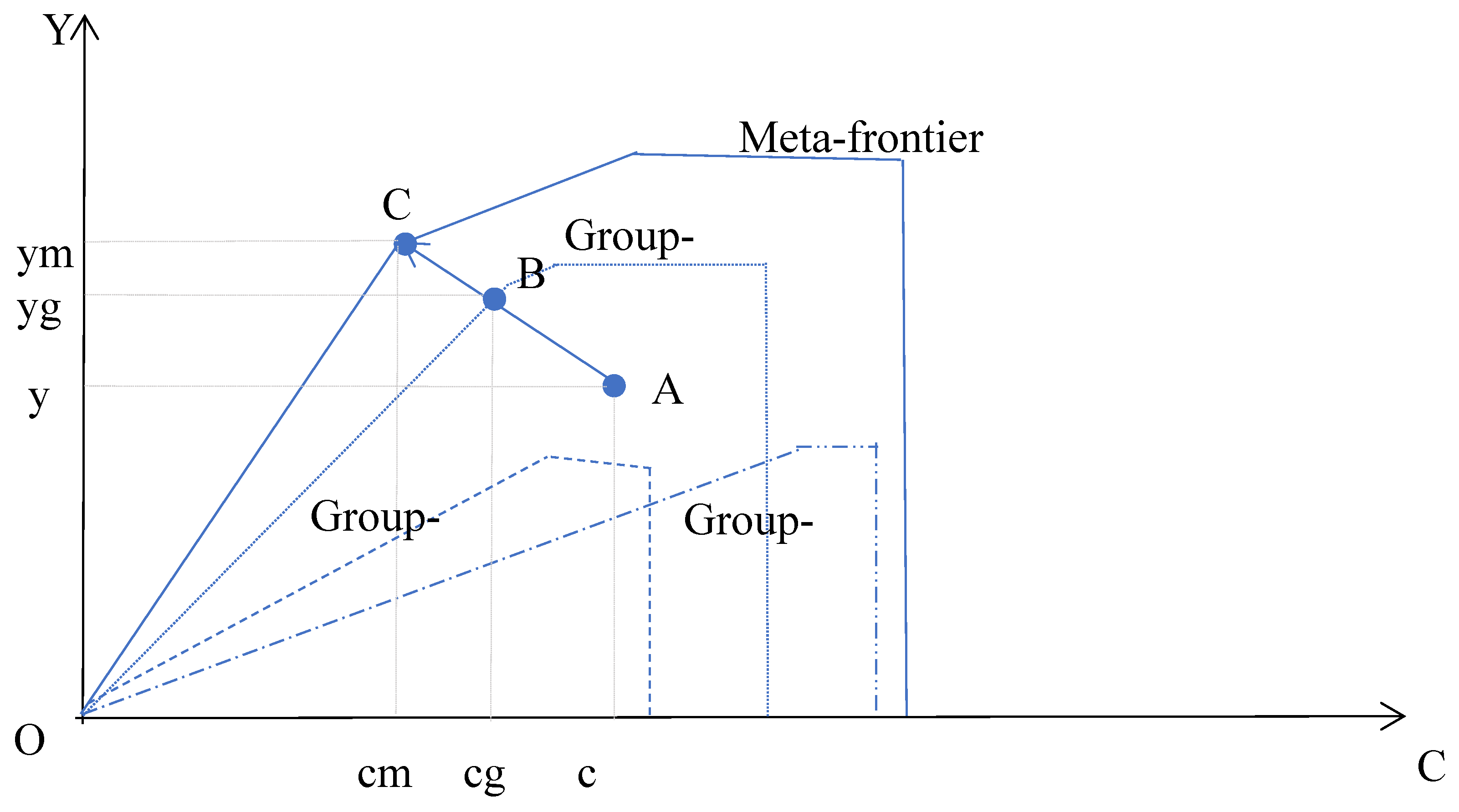
Based on the method of O’Donnell et al. (2008) [39], this study decomposes technical efficiency under meta-frontier technologies into within-group energy (or CO₂ emission) and meta-technology (also the technology gap ratio) performances. In this regard, the within-group energy (or CO₂ emission) performance reflects the frontier technologies in a specific set of relative efficiency of observed within-group technology. The meta-technology ratio shows relative gaps between group-frontier and meta-frontier. In Figure 1, we consider a simple example:

According to Figure 1, city A belongs to group-frontier 1 and its GRDP is Y with CO₂ emissions. Under the group frontier technologies, point B gives the target values for GRDP and CO₂ emissions as “yg” and “cg.” The Group-Frontier Total-Factor Carbon Emission Performance Index (GTCPI) is the ratio of potential CO₂ strength to actual CO₂ strength and thus, it can be measured the relative distance (ocg/oyg)/(oc/oy) in Figure 1. For the meta-frontier technologies, the Meta-Frontier Total-Factor Carbon Emission Performance Index (MTCPI) can be measured by the ratio (ocm/oym)/(oc/oy). In this way, we can get the technology gap between a specific meta-frontier and group-frontier technology in terms of CO₂ emission performance. The meta-technology of CO₂ performance MTCPI can be measured with the ratio (ocm/ocg)/(oyg/oym) and it can be written as follows:

$$MTCPI=\frac{ocm/oym}{oc/oy}=\left(\frac{ocg/oyg}{oc/oy}\right)\cdot \left(\frac{ocm}{ocg}\cdot \frac{oyg}{oym}\right)=GTCPI\times MTRCI.$$

(13)

Similarly, the decomposition can be expressed as follows:

$$MTEPI=GTEPI\times MTREI.$$

(14)

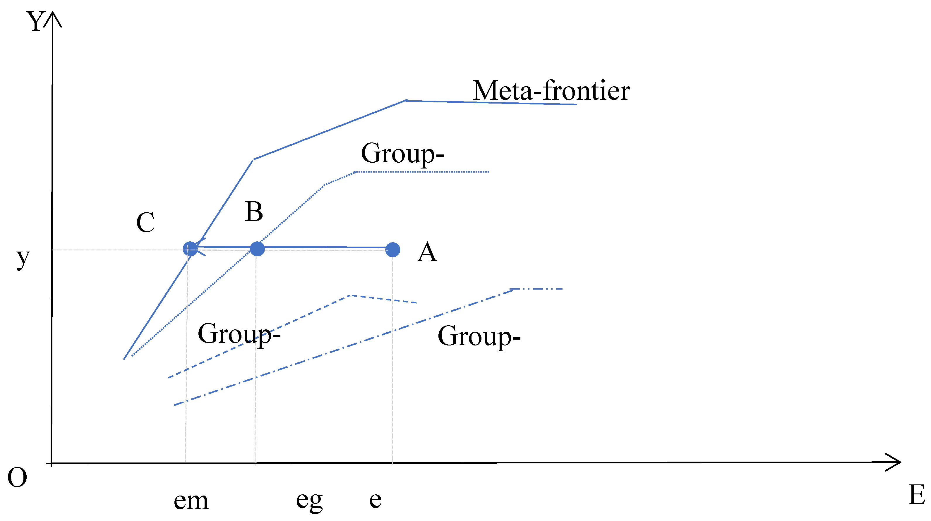
In the illustration in Figure 2, let us assume that there is a city in a specific group 1 that operates on point A. If a city is on point B, it means it is operating with group-frontier technology. Further, if the city can operate with meta-frontier technology, it will be on point C. The values of the Meta-Frontier Energy Potential Reduction Index (MEPRI) or Meta-Frontier Carbon Emission Potential Reduction Index (MCPRI) indicate the technology gap between group-frontier technology and meta-frontier technology. Higher values correspond to a smaller technology gap between group-frontier and meta-frontier technologies.

In this case, the potential gaps in energy reduction (PGERI) between group-frontier and meta-frontier can be defined as follows [16]:

$$PGERI=MEPRI-GEPRI.$$

(15)

Similarly, the potential gaps in carbon emission abatement (PGCRI) between group-frontier and meta-frontier can be defined as:

$$PGCRI=MCPRI-GCPRI.$$

(16)

3. Empirical Analysis

3.1. Data Collection

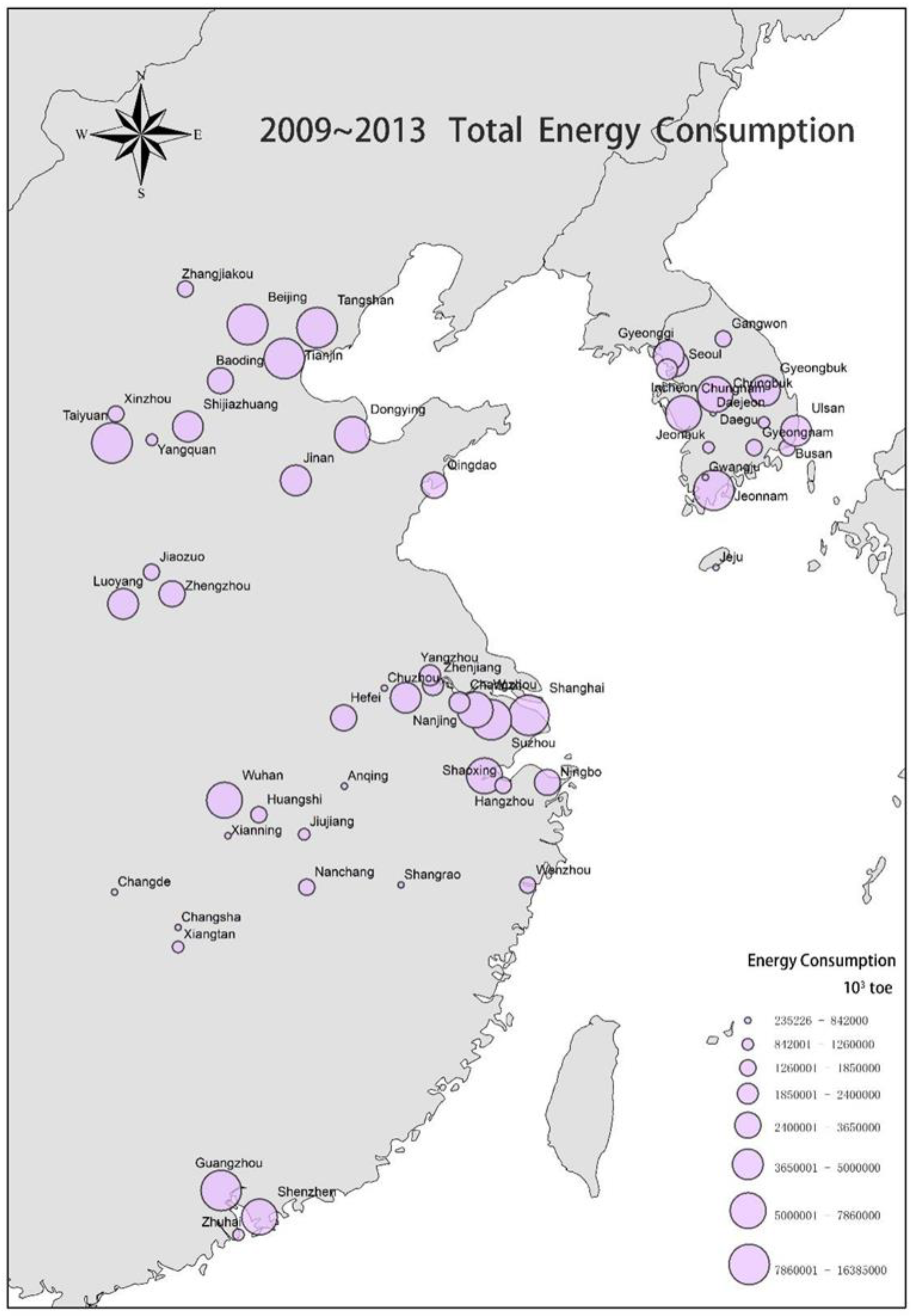
Based on the methodology described in Section 2 to examine energy and CO₂ performance, the data was collected from 16 cities in Korea, 23 cities from the eastern provinces of China, including Shandong, Jingjinji Metropolitan, Yangtze river delta, and Pearl river delta, and 18 cities from central China, including Taiyuan, Zhongyuan, Wanjiang, City Cluster surrounding Poyang Lake, Wuhan, and Greater Changsha Metropolitan cities. Figure 3 shows the location of China and Korea Cites and its energy use amount over five years.

The data was sourced from the annual data during 2009 to 2013 for the three groups: Korean Cities, Eastern Cities of China, and Central Cities of China. In Korea, the partly updated GHG emissions data for 2015 is available, but unfortunately, city-level data takes longer to be updated, so 2013 data is the most recent data we could get. In the DEA model, we selected two basic types of production inputs of capital and labor and another new input of energy consumption. Specifically, capital input is based on the perpetual inventory (stock) system used in Zhang et al. (2004) [40]. As capital stock cannot be directly obtained from any statistical yearbooks, following Young (2003) [41] and Zhang et al. (2017) [36], we calculated the capital stock as follows:

$$K_{n,t}=\frac{\Delta K_{n,t+1}}{({\delta }_n+g_n)},$$

(17)

where $K_{n,t}$ is the capital stock of city n at time t, $\Delta K_{n,t+1}$ denotes the investment in capital of city n at time t + 1, ${\delta }_n$ and $g_n$ is depreciation rate and GDP growth rate of city n respectively, the base year is 2009 so the price levels were adjusted to 2009 prices.

We calculated energy input based on energy consumption. For desirable output of GRDP, we take the GRDP of cities in China according to the data in Municipal Yearbook (CNKI (www.cnki.net)). The Korean data for labor, capital, energy, and GRDP was sourced from the Korea National Information Service (KOSIS) (KOSIS (http://kosis.kr/)). The nominal GRDP was adjusted using the 2009 GDP deflator. For undesirable output of CO₂ emissions, the pure CO₂ data for the Korean governments was unavailable. Hence, we followed the methodology used by Choi and Lee (2016) [17] for GHG emissions data for carbon dioxide (CO₂), which accounts for 78% of GHG emissions and other gases like nitrogen (N₂O), methane (CH₄), perfluorinated compounds (PFCs), sulfur hexafluoride (SF₆), and hydrofluorocarbons (HFCs) [42]. According to Xu et al. (2018) [43], the Chinese CO₂ data is cited from the database on http://www.ceads.net/. The basic descriptive statistics of inputs and outputs are shown in

Table 2. Descriptive statistics of production inputs and outputs.

Groups	Variable	Obs	Units	Mean	Std. Dev.	Min	Max
Korean cities (k)	Capital	80	106 US$	13,268.5	12,137.7	1547.4	61,079.7
	Labor	80	103 persons	1516.6	1523.6	283.0	5988.0
	Energy	80	103 toe	524,309.7	439,220.6	39,525.3	1,642,058.0
	Desirable outputs GRDP	80	106 US$	64,757.5	63,723.1	7959.7	248,914.0
	Undesirable output CO2	80	106 ton	31.5	27.9	2.8	118.3
Eastern cities of China (e)	Capital	115	106 US$	34,924.2	20,944.4	5356.4	117,953.8
	Labor	115	103 persons	5075.0	2616.8	1015.7	11,410.0
	Energy	115	103 toe	1,112,443	805,213.1	176,860.5	3,430,065.0
	Desirable outputs GRDP	115	106 US$	43,736.4	32,125.8	6634.7	131,308.6
	Undesirable output CO2	115	106 ton	94.4	62.8	11.1	310.3
Central cities of China (c)	Capital	90	106 US$	18,971.2	15,601.6	3163.6	69,947.6
	Labor	90	103 persons	2841.5	1481.2	582.8	5380.9
	Energy	90	103 toe	448,017.9	471,922.9	79,687.4	2,038,335.0
	Desirable outputs GRDP	90	106 US$	14,698.3	12,397.4	2890.7	53,272.8
	Undesirable output CO2	90	106 ton	51.0	47.0	9.5	209.8

Sources: Greenhouse Gas Inventory and Research Center of Korea (http://www.gir.go.kr), KOSIS (http://kosis.kr/), Municipal Yearbook (www.cnki.net), China Emission Accounts Datasets (http://www.ceads.net/).

.

As Table 2 shows, there are large variations across the three groups in all five variables. We can take Mean as an example. For inputs, the mean of the eastern city group of China (e) is the highest among the three groups. The Korean city group (k) has the lowest mean for capital and labor input, but its mean for energy consumption is more than that of the central city group of China (c). For desirable output of GRDP, the mean for the Korean city group has the highest value with the lowest CO₂ emissions mean.

3.2. Empirical Results

3.2.1. Carbon Emission Performance Indices

Our empirical test begins with the development of carbon emission and energy performance indices under group-frontier technologies to investigate whether there are significant differences in performance indices across groups and across cities.

Table 3. Energy and CO₂ emission performance under group-frontier technologies.

Variable	GTCPI				GTEPI
	Mean	Std. Dev.	Min	Max	Mean	Std. Dev.	Min	Max
k	0.931	0.071	0.724	1.000	0.913	0.078	0.645	1.000
e	0.927	0.100	0.577	1.000	0.917	0.110	0.539	1.000
c	0.912	0.092	0.578	1.000	0.824	0.204	0.287	1.000

presents the energy and CO₂ emission performance indices across groups under group-frontier. Figure 4, Figure 5 and Figure 6 illustrate the city-level energy and CO₂ emission performance indices for five years.

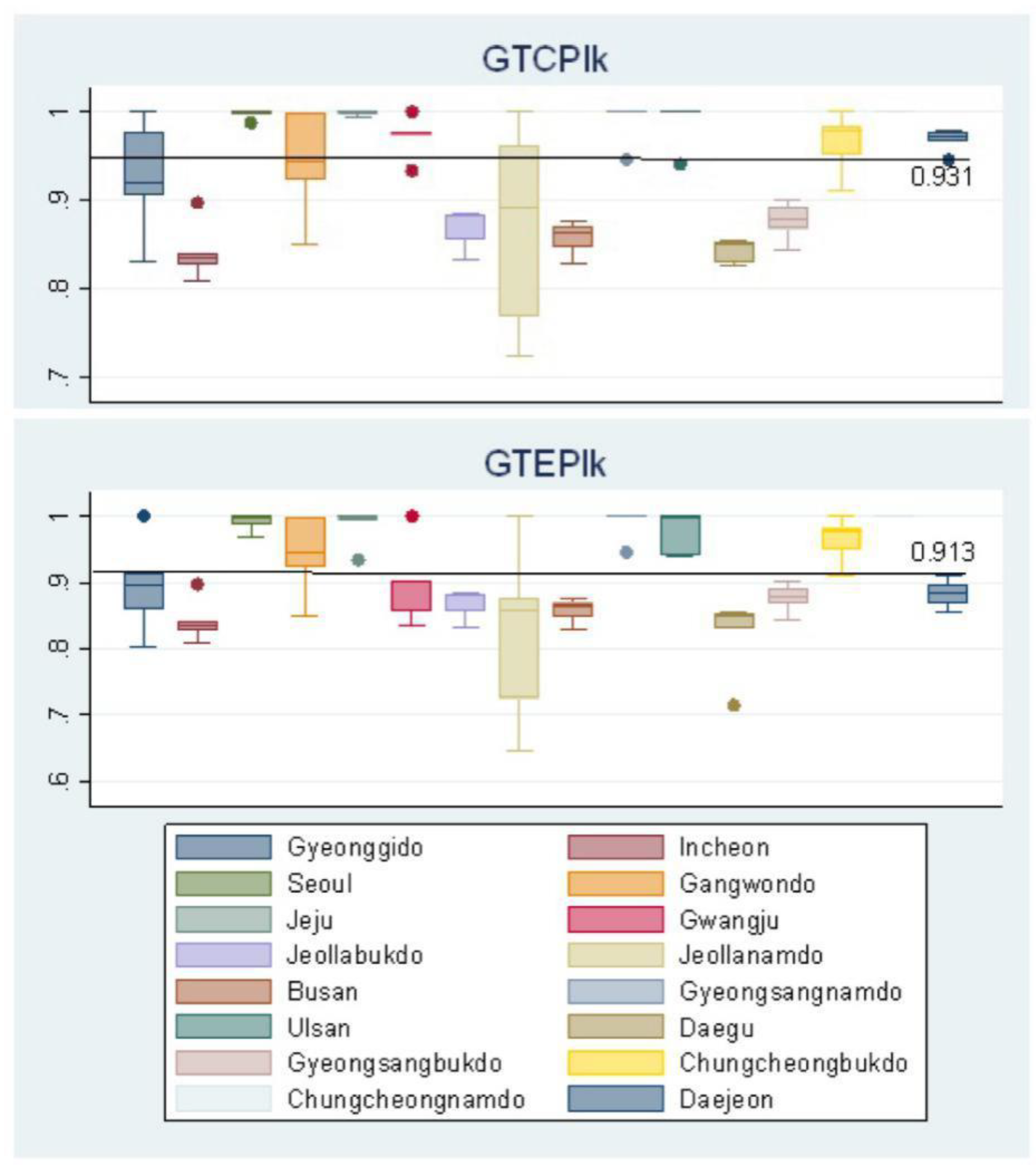
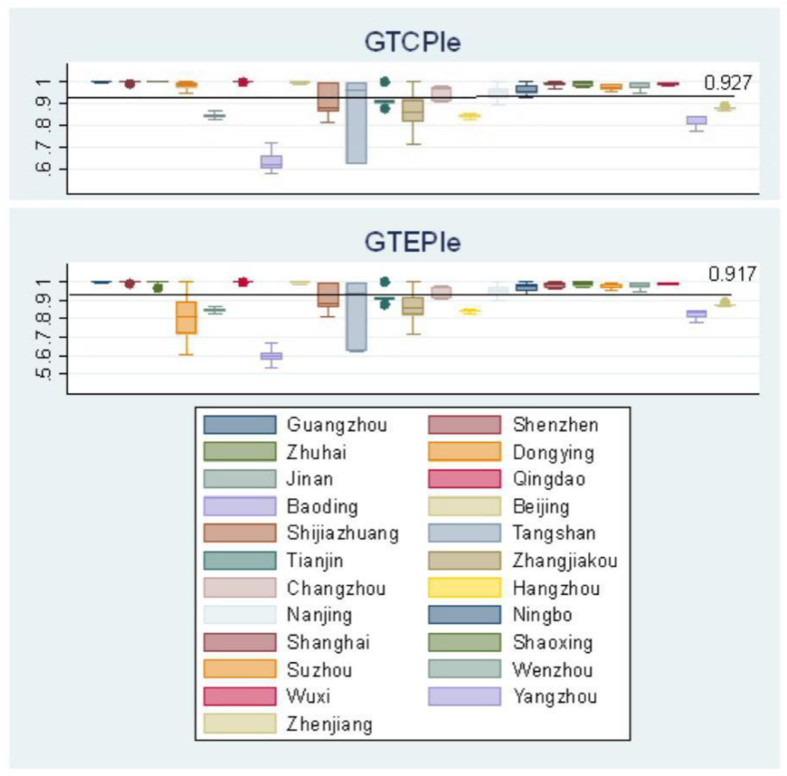
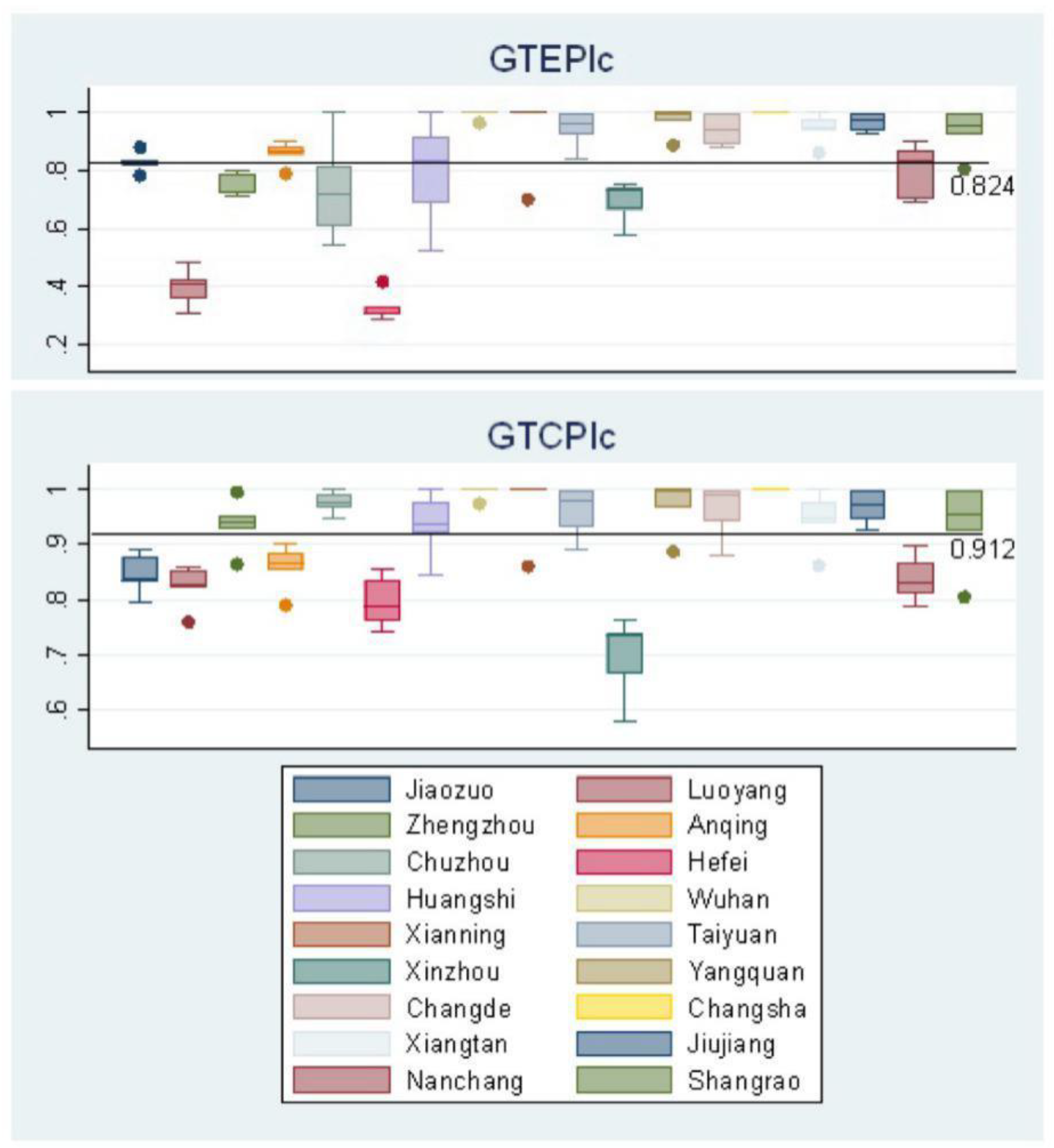
First, we consider the CO₂ emission performance under group-frontier technologies. Table 3 shows that the average GTCPI value for Korean cities (k) is 0.931 indicating that, on average, Korean cities can reduce their CO₂ intensity by 6.9% if all these cities are on the group frontier. The standard deviation for Korean cities is the lowest implying the smallest technical differences within-group. As for the eastern cities of China (e), the GTCPI value ranges from 0.577 to 1.000, with the average GTCPI value of 0.927. This suggests that the eastern cities of China can improve their CO₂ emission performance by 7.3%, if all within-group cities can operate with group-frontier technologies. In addition, the highest standard deviation of GTCPI for the eastern cities of China shows the greatest variance in within-group technology gaps. Therefore, the eastern cities of China have the greatest potential to improve their CO₂ emissions performance. The GTCPI value ranges from 0.578 to 1.000, with average GTCPI value of 0.912, which implies that the central cities of China can improve their CO₂ emissions performance by 8.8%, if all within-group cities can operate with group-frontier technologies.

Next, we consider GTCPI at city levels. For the agglomerated Korean cities, as Figure 4 shows, the value of GTCPIk for five years ranges from 0.724 to 1. Seoul, Jeju, Chungnam, and Ulsan show a higher performance than the other cities. Jeonnam shows the lowest value, implying that Jeonnam has the greatest potential for carbon emission performance improvement. For the eastern agglomerated cities of China, Guangzhou, Shenzhen, Zhuhai, Qingdao, Beijing, and Shanghai attain unity more than three times, indicating that they are at best practice CO₂ emission performance. Baoding has the lowest GTCPIe value, implying that it has the greatest potential for CO₂ emission performance improvements. For the central cities of China, as shown in Figure 6, only Wuhan, Xianning, Yangquan, and Changsha cities attain unity thrice in five years. Xinzhou shows the lowest GTCPI value, implying that it has the greatest potential for CO₂ emission performance improvements.

3.2.2. Energy Performance Indices

We analyzed the energy performance indices under group-frontier technologies. As shown in Table 3, the Group-Frontier Total-Factor Energy Performance Index (GTEPI) value for Korean cities (k) ranges from 0.654 to 1.000 with an average value of 0.913 indicating that, on average, Korean cities can improve their energy performance by approximately 8.7% if all within-group agglomerated cities perform on the best practice group-specific technologies. The standard deviation for Korean cities is the lowest, implying the smallest technology gap within-group. As for the eastern cities of China (e), the GTEPI value ranges from 0.539 to 1.000, with average GTEPI value of 0.917, which suggests that the eastern cities of China can improve energy performance by approximately 8.3%. The GTEPI value for the central cities of China ranges from 0.287 to 1.000, with average GTEPI value of 0.824. These results suggest that the central cities of China can improve energy performance by approximately 17.6%, if all within-group cities operate on group-frontier technologies. Among the three groups, the highest standard deviation of GTEPI is for the central cities of China, implying the greatest within-group technology gaps. Therefore, the central cities of China have the greatest potential to improve energy performance.

Next, we consider GTEPI at city level. As shown in Figure 4, Figure 5 and Figure 6, there are significant variations in energy performance indices at city level. For the Korean cities, as shown in Figure 4, the value of GTEPI for five years ranges from 0.645 to 1. Seoul, Jeju, Chungnam, and Ulsan show a higher performance than other cities. Jeonnam shows the lowest value, implying Jeonnam has the greatest potential for energy performance improvement. For the eastern cities of China, as shown in Figure 5, Guangzhou, Shenzhen, Zhuhai, Qingdao, Beijing, and Shanghai cities attain unity more than thrice, indicating that they are at best practice energy performance. Baoding shows the lowest GTCPIe value, implying that it has the greatest potential for energy performance improvements. For the central cities of China, as shown in Figure 6, only Wuhan, Xianning, Yangquan, and Changsha cities attain unity more than thrice in five years. Xinzhou shows the lowest GTCPI value implying that it has the greatest potential for energy performance improvements within this group.

Figure 4, Figure 5 and Figure 6 show that the average GTCPI value of 0.931 is higher than the average GTEPI value (0.913), indicating that the Korean cities show a better CO₂ emission performance than energy performance. In addition, we also found that cities with high CO₂ emission performance also have high energy performance. Further, we found similar results for the eastern and central cities of China. These results are not surprising since we assumed fixed CO₂ emission factors of energy in our research.

From the results, we also found that the average for GTCPI and GTEPI values shows an uptrend between 2009 and 2012, but it shows a mild downtrend in the year 2013, which is consistent with results obtained from other research, such as Lee and Choi (2018) [17]. Thus, we can say that since the target management system (TMS) was implemented in 2009, the strict environmental regulation has increased efficiency and encouraged innovation for a more environmentally-friendly production process. Unfortunately, the successor of President Park Geun-hye changed the paradigm from “green growth” to “creative economy” in 2013. As a result, environmental policies became passive and lax compared to the policies of the former president Lee Myung-bak’s government. We find that the average for GTCPI and GTEPI value shows a downtrend from 2009 to 2010, uptrend in 2011, and a downtrend again in 2012 to 2013, which is consistent with other research too [44].

According to the state council regulations, 2010 was the deadline for reporting the targets of the 11th five-year plan in China. If the local government fails to fulfill its task of energy conservation and emission reduction during the 11th five-year plan, relevant leaders are to be held accountable or even removed from their official position.

3.3. Total-Factor and Single-Factor Performance Indices

Next, we compared the total and single factor performance indices, as shown in

Table 4. Total-factor and single-factor performance indices.

Agglomerated Cities	Total-factor GTEPI	Single-factor GPEPI	Total-factor GTCPI	Single-factor GPCPI
Korean Cities (k)	0.913	0.882	0.931	0.885
Eastern Cities of China (e)	0.917	0.918	0.927	0.919
central Cities of China (c)	0.824	0.831	0.912	0.883

. We set the weight vector as (0,0,1/3,1/3, and 1/3) in Equation (8), to measure the single (or pure) factor energy and CO₂ emission performance by fixing the capital and labor inputs. There should be no possibility of substitution between energy and other productive inputs (capital and labor). The average of the GTEPIk (GTCPIk) value is higher than that of the GPEPIk (GPCPIk) value, suggesting that the alternatives between energy and other production inputs contribute to improved energy and carbon performance. However, for the eastern and central cities of China, the GTEPI average is slightly lower than the GPEPI average, suggesting that the substitution between energy and other production inputs reduces energy performance. The results are not surprising as there is a regional gap between the three groups. In general, it requires a large initial capital stock to replace energy in the production process. The capital stock in Korea is quite limited, thus inhibiting the substitution of factors between energy and other production inputs. As a result, substitutability between production inputs is very limited in Korea. The result for the eastern and central cities of China illustrates the Chinese government’s erroneous policy of energy saving and power rationing again. Power rationing reduces productivity. The blind pursuit of rapid GDP growth by local policy makers has delayed the elimination of enterprises using outdated production capacity, leading to a reassessment of energy-saving targets and the local government resorting to forced power cuts to meet the targets. First, the mandatory “power rationing” disrupts the normal production of enterprises, destroys the ability of enterprises to use peak and valley regulations and other measures to save electricity. The production process of an enterprise is continuous, and orders received must be delivered on time. Forced switch-offs and power rationing leads to a short-term backlog of production tasks of enterprises, after which enterprises are bound to work overtime, resulting in a growth of power consumption and artificial power supply tension. Secondly, under the forced pressure of power limit, many enterprises are forced to abandon the power supply from the “power grid” and adopt “self-provided diesel power generation” to solve the pressing need to ensure that their production and business activities are not greatly affected. This not only wastes energy, but also causes serious damage to the national energy strategy.

In Section 3.4 and Section 3.5, we test for group-heterogeneity across cities, and find whether there are significant differences in CO₂ emission and energy performance across cities.

Table 5. Meta-frontier energy and CO₂ emission performance and the meta-technology gap.

Variable	Mean	Std. Dev.	Variable	Mean	Std. Dev.	Variable	Mean	Std. Dev.
MTREIk	1.000	0.000	MTREIe	0.294	0.074	MTREIc	0.400	0.187
MTRCIk	1.000	0.000	MTRCIe	0.408	0.112	MTRCIc	0.492	0.201
MTEPIk	0.913	0.078	MTEPIe	0.270	0.079	MTEPIc	0.323	0.173
MTCPIk	0.931	0.071	MTCPIe	0.378	0.113	MTCPIc	0.455	0.211

compares the meta-frontier energy and CO₂ emission performance. In addition, it also presents the MTREI and MTRCI values across cities. Table 8 gives the result of Pearson and Spearman correlation coefficients and the p-values.

3.4. Meta-Frontier Energy and CO₂ Emission Performance and the Meta-Technology Gap

The Korean cities have the highest average MTEPIk of 0.913 and average MTCPIk (0.931) in the three groups, signifying that they are relatively efficient in terms of energy performance and CO₂ emissions. In this case, if all the agglomerated cities adopt meta-frontier technology, the energy efficiency of the Korean cities can be improved by 8.7% and the carbon emission performance can be improved by 6.9%. We also found that the average MTCPIk value is higher than the average MTEPIk value, indicating that the Korean cities are relatively more efficient in CO₂ emissions than energy performance. In addition, MTCPIk shows the lowest standard deviation, which means there is the smallest intra-agglomerated city technology gap in CO₂ emissions performance. Since average MTREIk and MTRCIk values are equal to 1, it makes no difference in energy and CO₂ performance indices between meta-frontier and group-frontier. Therefore, the Korean cities play an important role for benchmarking under meta-frontier.

In contrast, the average MTEPIe value of 0.270 and average MTCPI value (0.378) for the eastern cities of China are the lowest, signifying the eastern cities of China are the least efficient in terms of energy or CO₂ emissions performance. Among the three groups, the eastern cities of China have the greatest potential to improve energy efficiency and they can increase their energy efficiency by 73%, if they adopt meta-frontier technologies in all cities. In this context, the CO₂ emission performance of eastern cities of China can also be improved by 62.2%. In addition, MTEPIe and MTCPIe show relatively low standard deviations, signifying a small within-group technical gap in energy and CO₂ performance. In contrast to the Korean cities, there are significant differences between meta-frontier and group-frontier in the eastern cities of China. The average MTREIe value is 0.294 and MTRCIe value is 0.408, implying that the eastern cities of China can improve their energy performance by 70.6% and CO₂ emission performance by 59.2% with meta-frontier technologies. In comparison, the average MTREIe is lower than the average MTRCIe value, indicating that meta-technology gaps are relatively severe for energy efficiency.

Meanwhile, the central cities of China show a medium average MTEPIc value of 0.323 and average MTCPIc value (0.455), signifying the energy and CO₂ performance of the central cities of China are more effective than the eastern cities of China. Given that all cities use cutting-edge technology, the central cities of China could increase their energy performance by 67.7% and carbon performance by 54.5%. The largest within-group efficiency gap is similar for the central and the eastern cities of China. The average MTREIc value of 0.400 and average MTRCIc value of 0.492, indicates that the central cities of China can improve their energy performance by 60% and CO₂ emission performance by 50.8% with meta-frontier technologies.

Next, we compare the efficiency gap from the agglomerated city perspective. For the Korean cities, the average GTEPIk is equal to the average MTEPIk, and the average GTCPIk is equal to the average MTCPIk. These results show there is no technical gap in Korea between the group-frontier and the meta-frontier between GTEPI and MTCPI. For the eastern cities of China, the average value of GTEPI is much higher than of MTEPI, and the average value of GTCPI is significantly higher than of MTCPI. These results imply a considerable technological gap in eastern China between the group-frontier and the meta-frontier technologies. Similar results were found in central cities of China. However, it needs to be mentioned here that because we chose city-level data instead of province-level data as the object of our study, we found that under meta-frontier technology, the central cities of China show a medium average in energy and CO₂ emission performance which is better than the eastern cities of China. These results suggest that group heterogeneity could exist across cities. Without taking heterogeneity into consideration, the energy efficiency index in the central and eastern region might be overestimated. It can also be observed that Korean cities play a more important role in the baseline for efficiency of the meta-frontier technology.

Finally, we compare efficiency gaps at city level. Since it is not easy for cities to catch up with energy conservation and emissions reduction, the central government needs to support the local governments to learn more from the benchmark cities on the meta-frontier. We used the benchmark information for 2009. The cities can learn from the benchmarking cases of effective DMU—each inefficient DMU can learn by matching to an efficient DMU called a “reference set.” When similar input and output structures are present, the reference set is assigned to the inefficient DMU. For an inefficient DMU to improve its efficiency, its input target should reach the value derived from Equation (18). Cities for benchmark under the VRS condition can be derived as:

Reference set’s input * λ = inefficient DMU’s input target.

(18)

The intercept value can be defined as the degree of influence of DMU on each inefficient DMU. For example, the target value of DMU 1, Gyeonggi = DMU 10 Gyeongnam (2012) * 0.031+ DMU 12 Daegu (2012) * 0.719+ DMU 15 Chungnam (2012) * 0.201 + DMU 16 Daejeon (2010) *0.019 + DMU 16 Daejeon (2012) * 0.030. In the same way, DMU 3 Seoul’s target value can come from the input value of DMU 3 Seoul (2009) * 1.000. The result of the benchmark information is shown in Appendix B. In this result, we find DMU 12 Daegu (2009) is the best DMU as it showed up 31 times as a reference set. This is because, among the 57 sample cities for this research, DMU 12 Daegu’s (2009) input and output structure would be similar to other inefficient DMUs. Efficient DMUs that are not reported as a benchmark set as much as DMU 12 Daegu (2009), imply that their input and output structure is different from other inefficient DMUs. With the benchmark information the inefficient DMU should learn from the cases of their allocated reference set.

3.5. Test for Group-Heterogeneity Across Agglomerated Cities

Since the cities in the three groups have large differences in their economic environment as well as production technology level, we conducted tests for group-heterogeneity across the three groups. The tests aimed to find out whether there are significant differences between energy and carbon emission performance across groups.

Table 6. Results of the Wilcoxon-Mann-Whitney U-test.

Null Hypothesis (H0)	Mann-Whitney U Statistic	p-Value
Mean (MTEPIk) = Mean (MTEPIe)	12,440 ***	0.000
Mean (MTEPIk) = Mean (MTEPIc)	10,310 ***	0.000
Mean (MTEPIe) = Mean (MTEPIc)	11,022 *	0.051
Mean (MTREIk) = Mean (MTREIe)	12,440 ***	0.000
Mean (MTREIk) = Mean (MTREIc)	10,440 ***	0.000
Mean (MTREIe) = Mean (MTREIc)	9857 ***	0.000
Mean (MTCPIk) = Mean (MTCPIe)	12,423 ***	0.000
Mean (MTCPIk) = Mean (MTCPIc)	10,112 ***	0.000
Mean (MTCPIe) = Mean (MTCPIc)	11,054 *	0.061
Mean (MTRCIk) = Mean (MTRCIe)	12,440 ***	0.000
Mean (MTRCIk) = Mean (MTRCIc)	10,440 ***	0.000
Mean (MTRCIe) = Mean (MTRCIc)	10,722 **	0.008

*** significant at the level of 0.1%, ** significant at the level of 1%, * significant at the level of 5%.

reports the results of the Wilcoxon-Mann-Whitney U-test. From Table 6, all indexes of MTEPI, MTREI, MTCPI and MTRCI, and all invalid assumptions can be rejected at a significant level of 5% as far as the group heterogeneity is concerned. These results indicate that there is group heterogeneity among the three groups in terms of energy and CO₂ emission performance.

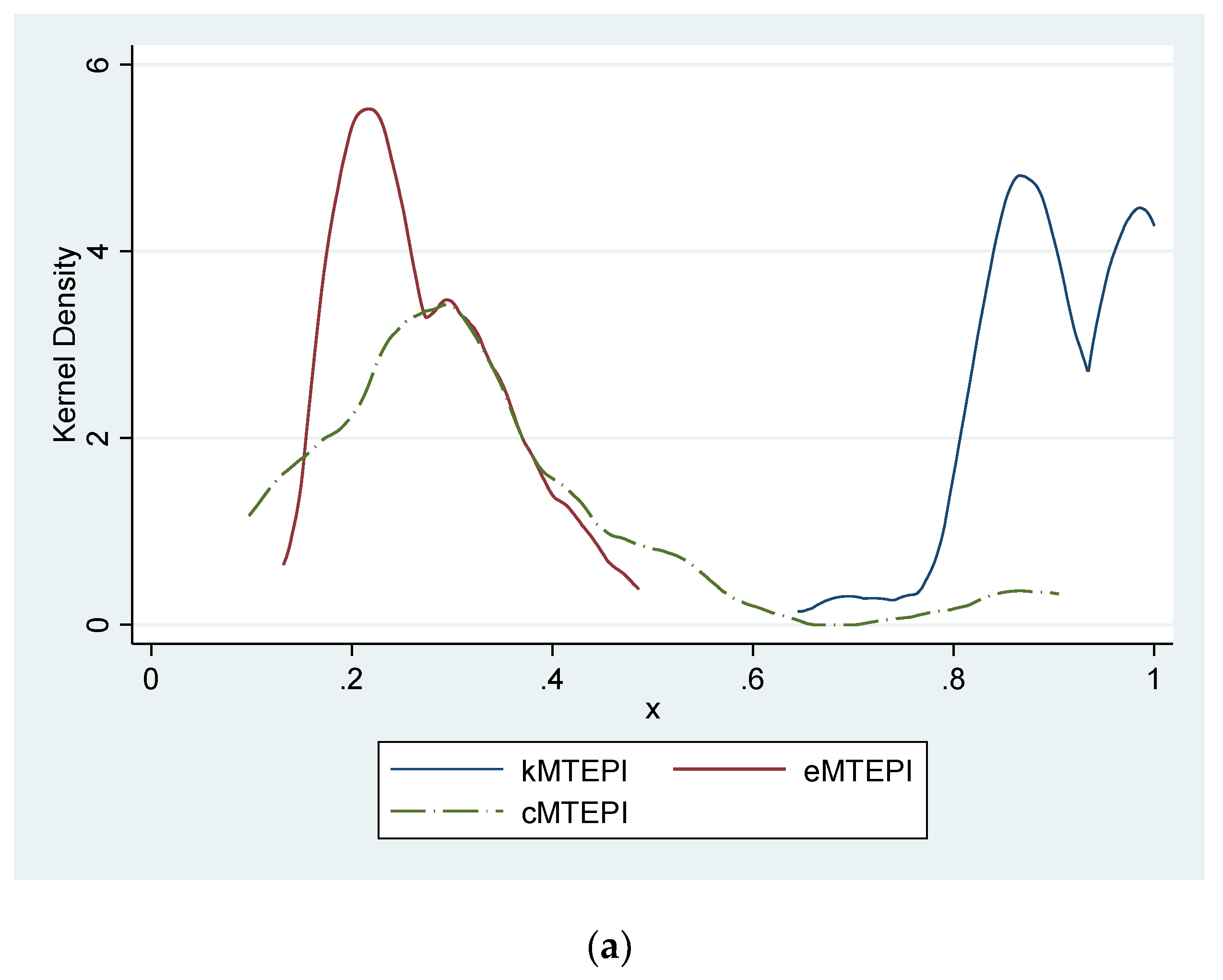
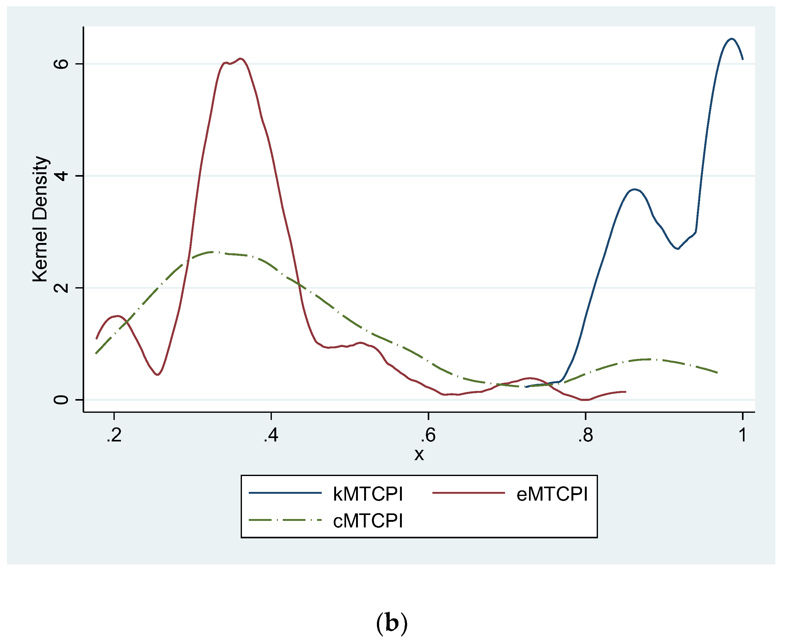
In addition, we used the Kolmogorov–Smirnov tests on MTEPI, MTREI, MTCPI, and MTRCI to determine any significant differences in Kernel density distribution.

Table 7. Results of the Kolmogorov–Smirnov test.

Indices	Null Hypothesis (H0)	K-S Statistic	p-Value
MTEPI	Distribution (Korean) = Distribution (East)	1.000 ***	0.000
	Distribution (Korean) = Distribution (Central)	0.944 ***	0.000
	Distribution (Central) = Distribution (East)	0.200 *	0.035
MTREI	Distribution (Korean) = Distribution (East)	1.000 ***	0.000
	Distribution (Korean) =Distribution (Central)	1.000 ***	0.000
	Distribution (Central) = Distribution (East)	0.314 ***	0.000
MTCPI	Distribution (Korean) = Distribution (East)	0.979 ***	0.000
	Distribution (Korean) = Distribution (Central)	0.844 ***	0.000
	Distribution (Central) = Distribution (East)	0.239 ***	0.006
MTRCI	Distribution (Korean) = Distribution (East)	1.000 ***	0.000
	Distribution (Korean) = Distribution (Central)	1.000 ***	0.000
	Distribution (Central)= Distribution (East)	0.264 ***	0.002

*** significant at the level of 0.1%, ** significant at the level of 1%, * significant at the level of 5%.

reports the results of the Kolmogorov–Smirnov test. In terms of the performance indexes of MTEPI, MTREI, MTCPI, and MTRCI, it was found that for the Kernel density distribution among three groups, all null hypotheses were rejected at a significant level of 5%. These results indicate that the Kernel density distribution proves the different density distribution for each other, supporting heterogeneity for all three groups (Figure 7).

Next, we tested the Spearman correlation coefficients. We found from

Table 8. Correlations between indices.

	GTCPI	GTEPI	MTCPI	MTEPI	MTRCI	MTREI
GTCPI	1.000
GTEPI	0.9216 ***	1.000
	(0.000)
MTCPI	0.3769 ***	0.3497 ***	1.000
	(0.000)	(0.000)
MTEPI	0.3126 ***	0.3350 ***	0.7805 ***	1.000
	(0.000)	(0.000)	(0.000)
MTRCI	0.1166 *	0.1213 *	0.9507 ***	0.7278 ***	1.000
	(0.049)	(0.041)	(0.000)	(0.000)
MTREI	0.033	0.007	0.7073 ***	0.9200 ***	0.7310 ***	1.000
	(0.585)	(0.905)	(0.000)	(0.000)	(0.000)

*** significance level is 0.1%, * significance level is 5%.

that most of the performance indicators have a positive correlation. As expected, MTEPI shows a high correlation with MTCPI, while MTREI shows a high correlation with MTRCI, since carbon emissions are calculated based on energy-type carbon emission factors. In contrast, the results do not support a positive correlation between GTEPI (GTCPI) and MTREI, suggesting that there is no significant correlation between the group-frontier performance index and the meta-frontier energy performance technology index, but there is a small one between the group-frontier performance index and the meta-frontier CO₂ emission performance technology index.

3.6. Abatement Potential for International Cooperation

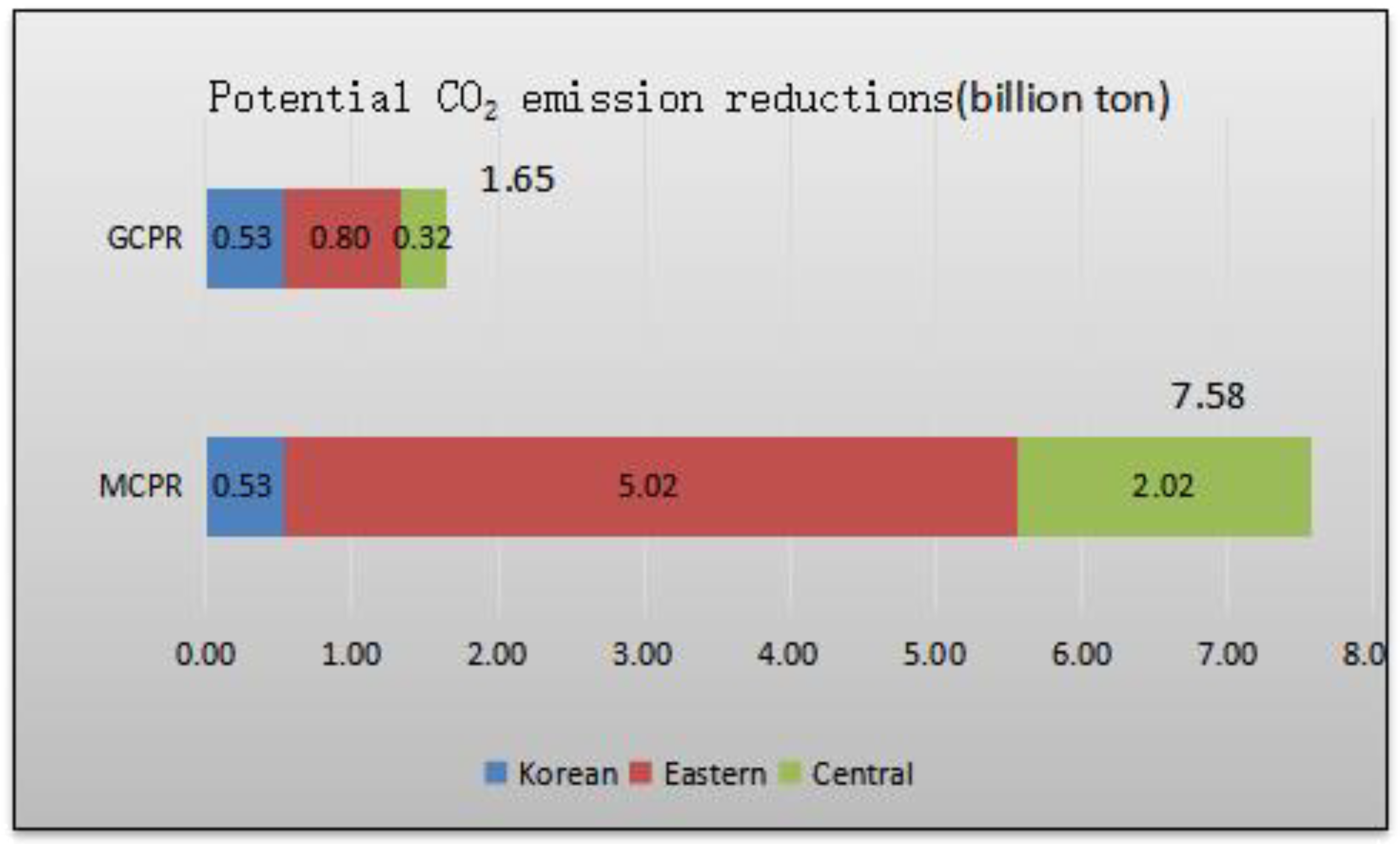
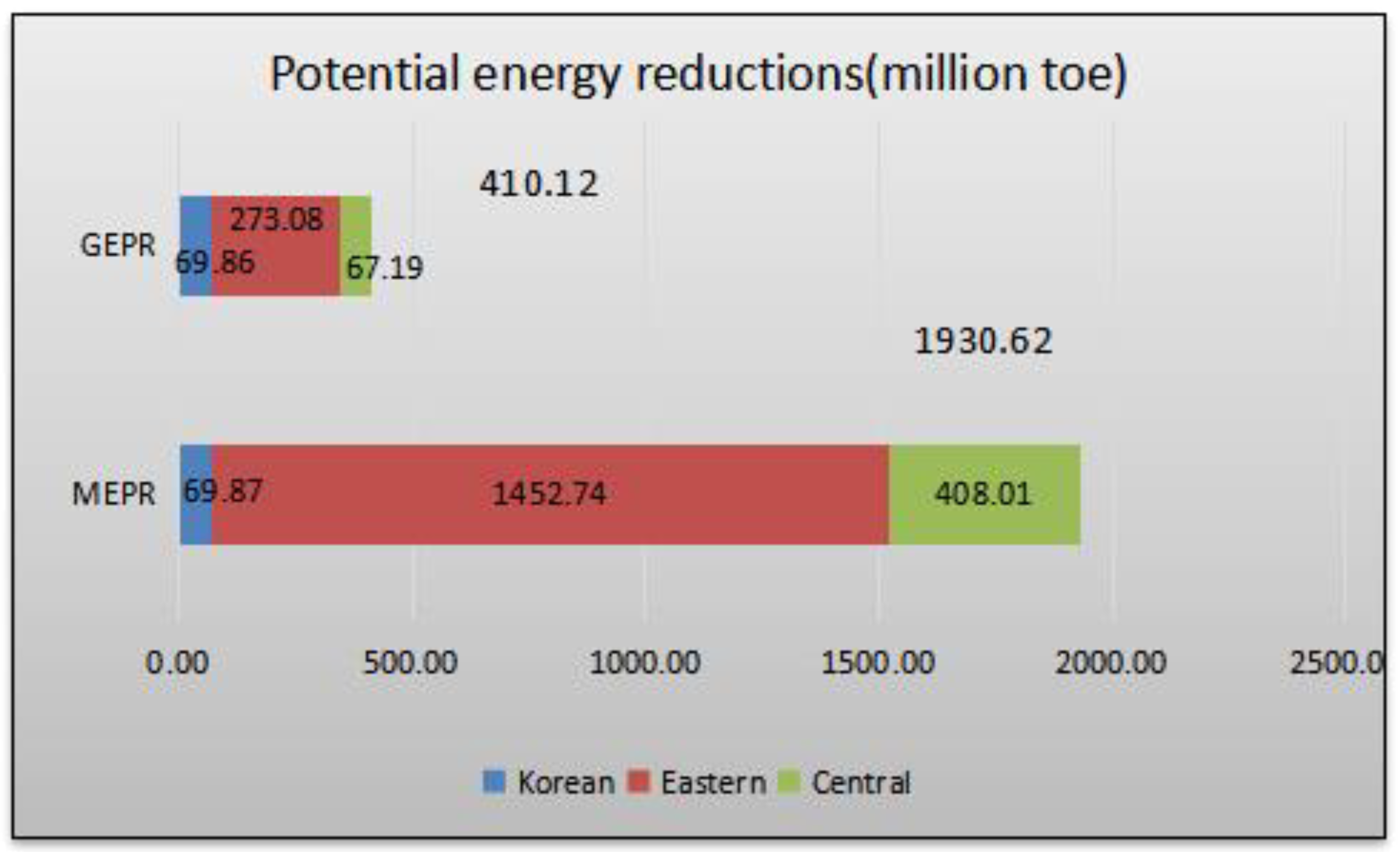
Finally, we analyzed the potential of energy and carbon emission abatement for international cooperation between China and Korea. Our purpose was to investigate whether cooperative policies can contribute significantly to energy consumption and carbon emission abatement. Figure 8 and Figure 9 demonstrate the potential of carbon emission abatement across the group-frontier and meta-frontier technologies. We find there will be huge potential CO₂ emission and energy reductions when all agglomerated cities can be on meta-frontier technologies. From 2009 to 2013, the Korean cities, and the eastern and northern Chinese could reduce CO₂ emissions by 0.53, 5.02 and 2.02 billion tons, respectively—a total reduction of 7.58 billion tons of CO₂ emissions for the five years if Korea and China proactively collaborate with each other. The Korean cities and the eastern and central Chinese cities can reduce their energy consumption by 69.86, 1452.74, and 408.01 million toe, respectively—a total reduction of 1930.62 toe energy for the five years.

4. Conclusions

China, the world’s largest energy consumer and carbon emitter, and Korea, another heavy emitter, have set ambitious emissions reduction targets of 60% to 65% per unit of GDP and 37% reduction below the business as usual (BAU) levels till 2030 based on 2005 levels, by China and Korea, respectively. The northeast Asian region is a dynamic region in both its economic activities as well as environmental policies. As the saying goes, “without the lips, the teeth feel the cold.” China and South Korea should be intimately interdependent on each other for the effects of environmental policies.

Therefore, as neighboring countries, it is imperative for both governments to develop cooperative policies to curb energy consumption and CO₂ emissions in the region. However, establishing effective policy tools requires more complicated and yet systematic information about energy efficiency, CO₂ emission performance, and energy (CO₂ emission) reduction potential. China is a transitional economy with huge regional disparities and so, the Chinese government needs to pay more attention to their agglomerated cities. In the same way, Seoul has almost 50% of the Korean population, resulting in complex environmental issues from the excessive urbanization. To solve these environmental issues in the metropolitan cities, this study utilizes a GMNDDF of energy efficiency, CO₂ emission performance, and technology gap from a regional perspective. Our main findings are as follows:

First, in terms of energy efficiency and CO₂ emission performance, significant group heterogeneity exists in the three groups. Empirical results show significant differences among groups in energy efficiency, CO₂ emission performance, and meta-technology gaps. Nonetheless, to answer the question whether there is potential for international cooperation, we employed regional heterogeneity in our model. The Korean cities can play a leading role with benchmark efficiency level of the meta-frontier technology, as there are no meta-technology gaps in Korea at least. However, as far as the eastern and central cities of China are concerned, there is a considerable meta-technical gap between the group-frontier and the meta-frontiers. GTCPI and GTEPI values show an uptrend between 2009 and 2012, but a mild downtrend in 2013 in Korea, because the new President Park Geun-hye changed the Korean paradigm from “green growth” to “creative economy” and hence, environmental policies became more lax under the current administration. For the eastern and central cities of China, the average values for GTCPI and GTEPI show a downtrend in 2009 to 2010, increase in 2011, and downtrend again in 2012 to 2013, implying that the power cuts that plague China is the wrong policy, and sudden power outages are not conducive to business operations as it results in reduced production efficiency.

Second, there is no significant difference between total-factor and single-factor performance indices in the Korean cities, since Korea requires extensive labor and land resources to replace energy in the production process, which are quite limited. This inhibits the substitution of factors between energy and other production inputs. As a result, substitutability between production inputs is very limited in Korea. The eastern and central cities of China need technology, while the Korean agglomerated cities need labor and land resources. This illustrates that the Chinese government needs to restructure the production scale in the cities by learning from benchmark cities, and the Korean government needs to increase its production scale. They can also encourage enterprises to set up factories in China.

Third, three groups can make a huge contribution to reduce energy and CO₂ emissions by “catching up.” It is important for the local governments to remove barriers and regulations that limit flow of production inputs and encourage investment in advanced meta-frontier technologies, especially in cities with low energy efficiency and low CO₂ performance. In this way, China can significantly reduce its carbon emissions.

Fourth, many cities in China could enhance their environmental performance by international cooperation. There are several benchmarking cases for the possible arrangement of the cooperative activities for CO₂ emissions abatement. For example, Daegu (2009) is the best DMU as it shows up 31 times as a reference set for Chinese cities to emulate. With the benchmark information, the inefficient DMUs should be developed to enhance the learning effect on the cases of their allocated reference sets.

We demonstrate even if the eastern cities of China are much better in their environmental performance as a group, they are still inferior to the central cities of China. Moreover, all central and eastern cities of China lag far behind in environmental performance compared to the Korean cities, implying that the regional cooperation between cities in Korea and China could enhance performance. Many Memoranda of Understanding (MOUs) between cities in China and Korea have been signed for cooperation. This study showed that verbal commitment alone is not helpful for sustainable performance. Instead we show that the comparative city level analysis that could enhance the benchmarking cities among the two countries.

References

- BP. BP Statistical Review of World Energy. 13 June 2018. Available online: http://www.bp.com/statisticalreview (accessed on 30 June 2018).
- Sorrell, S. Reducing energy demand: A review of issues, challenges and approaches. Renew. Sustain. Energy Rev. 2015, 47, 74–82. [Google Scholar] [CrossRef] [Green Version]
- Ning, Y.; Miao, L.; Ding, T.; Zhang, B. Carbon emission spillover and feedback effects in China based on a multiregional input-output model. Resour. Conserv. Recycl. 2019, 141, 211–218. [Google Scholar] [CrossRef]
- Park, H.; Hong, W. Korea’s emission trading scheme and policy design issues to achieve market-efficiency and abatement targets. Energy Policy 2014, 75, 73–83. [Google Scholar] [CrossRef]
- Chavez, A.; Ramaswami, A. Progress toward low carbon cities: Approaches for transboundary GHG emissions’ foot printing. Carbon Manag. 2014, 2, 471–482. [Google Scholar] [CrossRef]
- Hoornweg, D.; Sugar, L.; Gomez, C.L.T. Cities and greenhouse gas emissions: Moving forward. Environ. Urban. 2011, 23, 207–227. [Google Scholar] [CrossRef]
- Kennedy, C.; Steinberger, J.; Gasson, B.; Hansen, Y.; Hillman, T.; Havranek, M.; Pataki, D.; Phdungsilp, A.; Ramaswami, A.; Mendez, G.V. Methodology for inventorying greenhouse gas emissions from global cities. Energy Policy 2010, 38, 4828–4837. [Google Scholar] [CrossRef]
- Kennedy, C.; Demoullin, S.; Mohareb, E. Cities reducing their greenhouse gas emissions. Energy Policy 2012, 49, 774–777. [Google Scholar] [CrossRef]
- Wang, H.; Zhang, R.; Liu, M.; Bi, J. The carbon emissions of Chinese cities. Atmos. Chem. Phys. 2012, 12, 6197–6206. [Google Scholar] [CrossRef]
- Li, A.; Hu, M.; Wang, M.; Cao, Y. Energy consumption and CO2 emissions in Eastern and Central China: A temporal and a cross-regional decomposition analysis. Technol. Forecast. Soc. Chang. 2016, 103, 284–297. [Google Scholar] [CrossRef]
- Kim, K.; Kim, Y. International comparison of industrial CO2 emission trends and the energy efficiency paradox utilizing production-based decomposition. Energy Econ. 2012, 34, 1724–1741. [Google Scholar] [CrossRef]
- Lin, B.Q.; Du, K.R. Technology gap and China’s regional energy efficiency: A parametric meta-frontier approach. Energy Econ. 2013, 40, 529–536. [Google Scholar] [CrossRef]
- Bian, Y.W.; He, P.; Xu, H. Estimation of potential energy saving and carbon dioxide emission reduction in China based on an extended non-radial DEA approach. Energy Policy 2013, 63, 962–971. [Google Scholar] [CrossRef]
- Wang, K.; Wei, Y.M. China’s regional industrial energy efficiency and carbon emissions abatement costs. Appl. Energy 2014, 130, 617–631. [Google Scholar] [CrossRef]
- Wang, Z.H.; Feng, C.; Zhang, B. An empirical analysis of China’s energy efficiency from both static and dynamic perspectives. Energy 2014, 74, 322–330. [Google Scholar] [CrossRef]
- Yao, X.; Zhou, H.C.; Zhang, A.Z.; Li, A.J. Regional energy efficiency, carbon emission performance and technology gaps in China: A meta-frontier non-radial directional distance function analysis. Energy Policy 2015, 84, 142–154. [Google Scholar] [CrossRef]
- Lee, H.; Choi, Y. Greenhouse gas performance of Korean local governments based on non-radial DDF. Technol. Forecast. Soc. Chang. 2018, 135, 13–21. [Google Scholar] [CrossRef]
- Farrel, M.J. The measurement productive efficiency. J. R. Stat. Soc. Ser. A Gen. 1957, 120, 253–290. [Google Scholar] [CrossRef]
- Charnes, A.; Cooper, W.W.; Rhodes, E. Measuring the efficiency of decision making units. Eur. J. Oper. Res. 1978, 2, 429–444. [Google Scholar] [CrossRef]
- Banker, R.D.; Charnes, A.; Cooper, W.W. Some Models for Estimating Technical and Scale Inefficiencies in Data Envelopment Analysis. Manag. Sci. 1984, 30, 9. [Google Scholar] [CrossRef]
- Tone, K. A Slacks-based Measure of Efficiency in Data Envelopment Analysis. Eur. J. Oper. Res. 2001, 130. [Google Scholar] [CrossRef]
- Färe, R.; Grosskopf, S.; Norris, M.; Zhang, Z. Productivity growth, technical progress, and efficiency change in industrialized countries. Am. Econ. Rev. 1994, 84, 66–83. [Google Scholar]
- Chung, Y. Directional Distance Functions and Undesirable Outputs. Ph.D. Dissertation, Southern Illinois University at Carbondale, Carbondale, IL, USA, 1996. [Google Scholar]
- Färe, R.; Grosskopf, S.; Pasurka, C.A. Environmental production functions and environmental directional distance functions. Energy 2007, 32, 1055–1066. [Google Scholar] [CrossRef]
- Oggioni, G.; Riccardi, R.; Toninelli, R. Eco-efficiency of the world cement industry: A data envelopment analysis. Energy Policy 2011, 39, 2842–2854. [Google Scholar] [CrossRef] [Green Version]
- Riccardi, R.; Oggioni, G.; Toninelli, R. Efficiency analysis of world cement industry in presence of undesirable output: Application of data envelopment analysis and directional distance function. Energy Policy 2012, 44, 140–152. [Google Scholar] [CrossRef]
- Fukuyama, H.; Weber, W.L. A directional slacks-based measure of technical inefficiency. Socio-Econ. Plan. Sci. 2009, 43, 274–287. [Google Scholar] [CrossRef]
- Barros, C.P.; Managi, S.; Matousek, R. The technical efficiency of the Japanese banks: Non-radial directional performance measurement with undesirable outpu. Omega 2012, 40, 1–8. [Google Scholar] [CrossRef]
- Tian, Y.H.; He, S.B.; Hu, S.Q. Re-estimation of total factor productivity growth in a region under environmental constraints:1998-2008. China’s Ind. Econ. 2011, 1. [Google Scholar] [CrossRef]
- Wang, B.; Wu, Y.R.; Yan, P.F. China’s regional environmental efficiency and total factor productivity growth. Econ. Res. 2010, 5. Available online: http://en.cnki.com.cn/Article_en/CJFDTOTAL-JJYJ201005008.htm (accessed on 30 June 2018).
- Pastor, J.T.; Knox Lovell, C.A. A Global Malmquist Productivity index. Econ. Lett. 2005, 88, 2. [Google Scholar] [CrossRef]
- Zhou, P.; Ang, B.W.; Wang, H. Energy and CO2 emission performance in electricity generation: A non-radial directional distance function approach. Eur. J. Oper. Res. 2012, 221, 625–635. [Google Scholar] [CrossRef]
- Choi, Y.; Zhang, N.; Zhou, P. Efficiency and abatement costs of energy-related CO2 emissions in China: A slacks-based efficiency measure. Appl. Energy 2013, 98, 198–208. [Google Scholar] [CrossRef]
- Färe, R.; Grosskopf, S. New Directions: Efficiency and Productivity; Springer: New York, NY, USA, 2005. [Google Scholar]
- Färe, R.; Grosskopf, S.; Lovell, C.A.K.; Pasurka, C. Multilateral productivity comparisons when some outputs are undesirable: A nonparametric approach. Rev. Econ. Stat. 1989, 71, 90–98. [Google Scholar] [CrossRef]
- Zhang, N.; Chen, Z.F. Sustainability characteristics of China’s Poyang Lake Eco-Economics Zone in the big data environment. J. Clean. Prod. 2017, 142, 642–653. [Google Scholar] [CrossRef]
- Chiu, C.R.; Liou, J.L.; Wu, P.I.; Fang, C.L. Decomposition of the environmental inefficiency of the meta-frontier with undesirable output. Energy Econ. 2012, 34, 1392–1399. [Google Scholar] [CrossRef]
- Battese, G.E.; Rao, D.S.P.; O’Donnell, C.J. A meta-frontier production function for estimation of technical efficiencies and technology gaps for firms operating under different technologies. J. Prod. Anal. 2004, 21, 91–103. [Google Scholar] [CrossRef]
- O’Donnell, C.J.; Rao, D.S.P.; Battese, G.E. Meta-frontier frameworks for the study of firm-level efficiencies and technology ratios. Empir. Econ. 2008, 34, 231–255. [Google Scholar] [CrossRef]
- Zhang, J.; Wu, G.Y.; Zhang, J.P. The Estimation of China’s provincial capital stock: 1952–2000. Econ. Res. J. 2004, 10, 35–44. [Google Scholar] [CrossRef]
- Young, A. Gold into base metals: Productivity growth in the People’s Republic of China during the reform period. J. Polit. Econ. 2003, 111, 1220–1261. [Google Scholar] [CrossRef]
- Olivier, J.G.J.; Schure, K.M.; Peters, J.A.H.W. Trends in global CO2 and total greenhouse gas emissions. PBL Netherlands Environmental Assessment Agency, 2017; p. 5. Available online: https://www.pbl.nl/sites/default/files/cms/publicaties/pbl-2017-trends-in-global-co2-and-total-greenhouse-gas-emissons-2017-report_2674.pdf (accessed on 28 October 2018).
- Xu, X.; Huo, H.; Liu, J.; Shan, Y.; Li, Y.; Zheng, H.; Guan, D.; Ouyang, Z. Patterns of CO2 emissions in 18 central Chinese cities from 2000 to 2014. J. Clean. Prod. 2018, 172, 529–540. [Google Scholar] [CrossRef]
- Wang, B.; Lai, P.H.; Yang, Y.S.; Yu, L.J. Study on the potential of energy efficiency and energy conservation and emission reduction in China considering the differences of natural environment. Rev. Ind. 2016. (In Chinese). Available online: http://www.cnki.com.cn/Article/CJFDTotal-TQYG201601008.htm (accessed on 28 October 2018).
Figure 1.
Meta-frontier CO2 emission performance index and its decomposition.