Multi-Objective Robust Scheduling Optimization Model of Wind, Photovoltaic Power, and BESS Based on the Pareto Principle

 ,
,
Abstract
:1. Introduction
2. System Output Model
2.1. Wind and Photovoltaic Power Output Model
2.1.1. Wind Power Output Model
2.1.2. Photovoltaic Power Model
2.2. BESS Output Model
3. System Robust Scheduling Model
3.1. Objective Function
3.1.1. System Operation Cost
3.1.2. System Carbon Emissions
3.2. Constraint Conditions
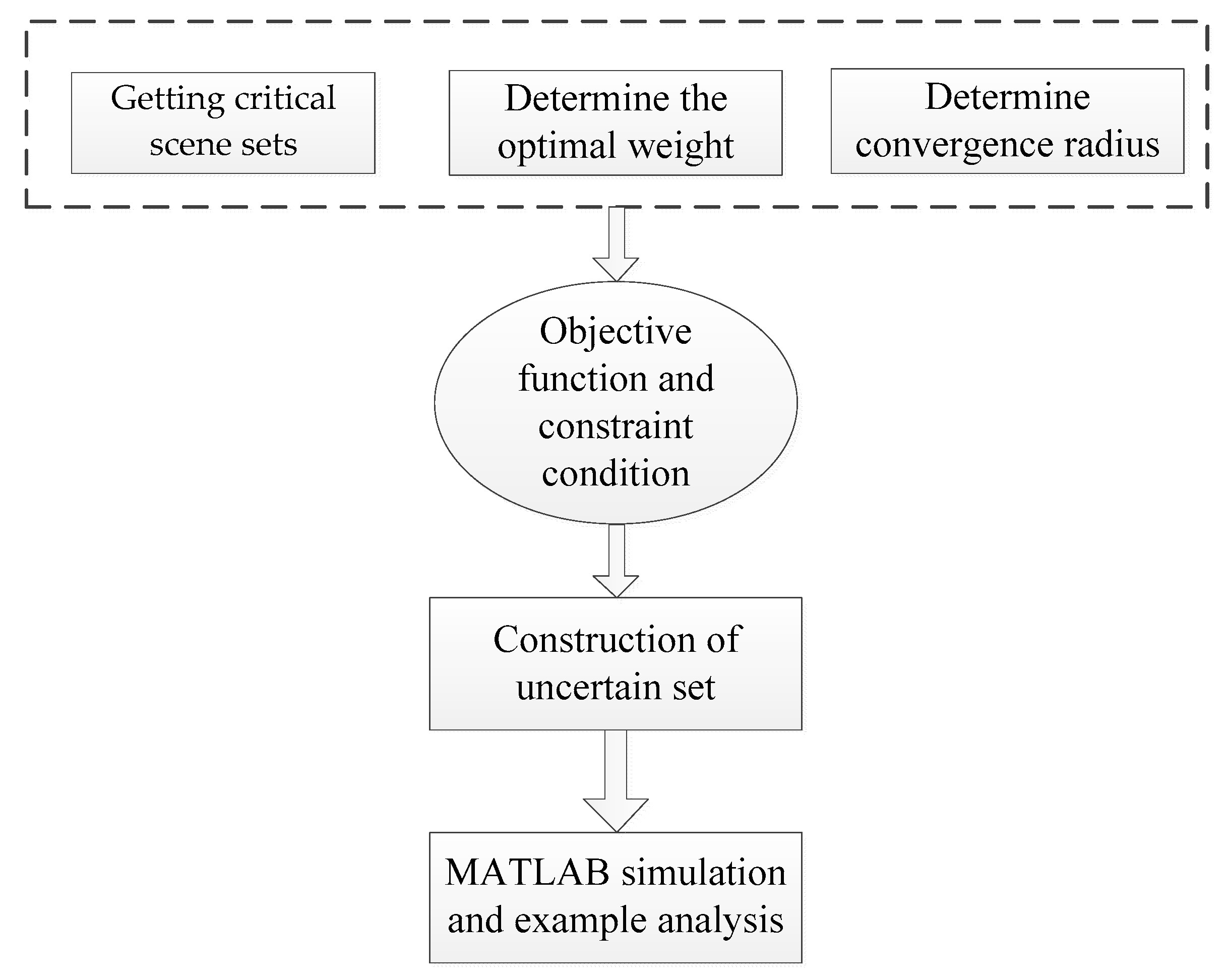
3.3. Uncertainty Set
3.4. Solving Algorithm
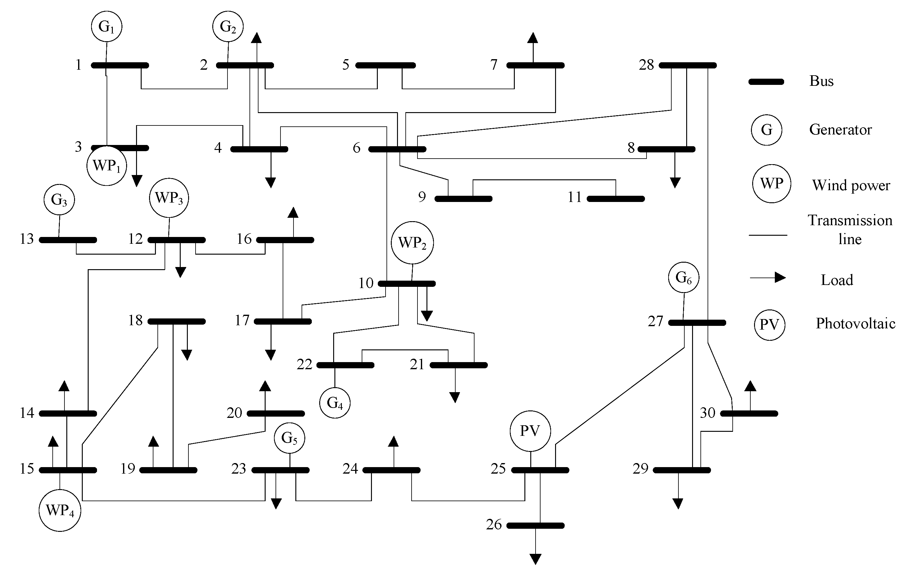
4. Simulation Studies
4.1. Simulation Scenario Setting
4.2. Basic Data
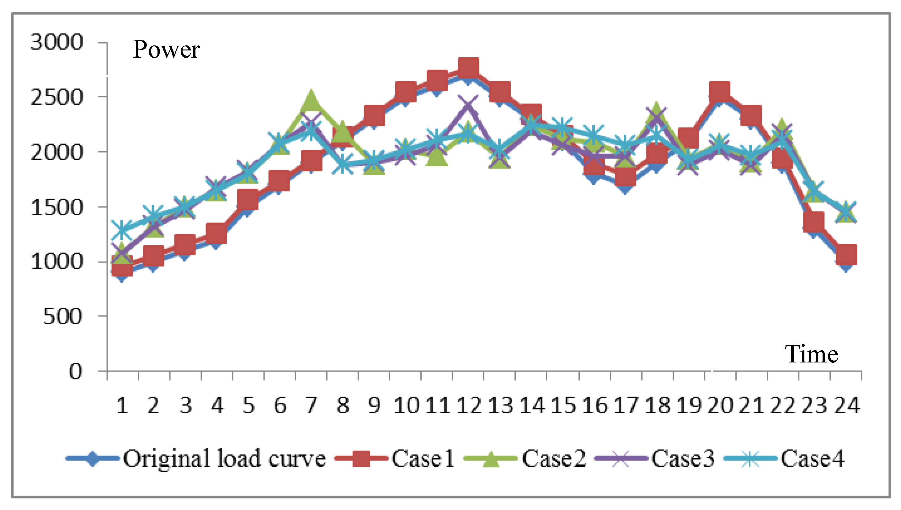
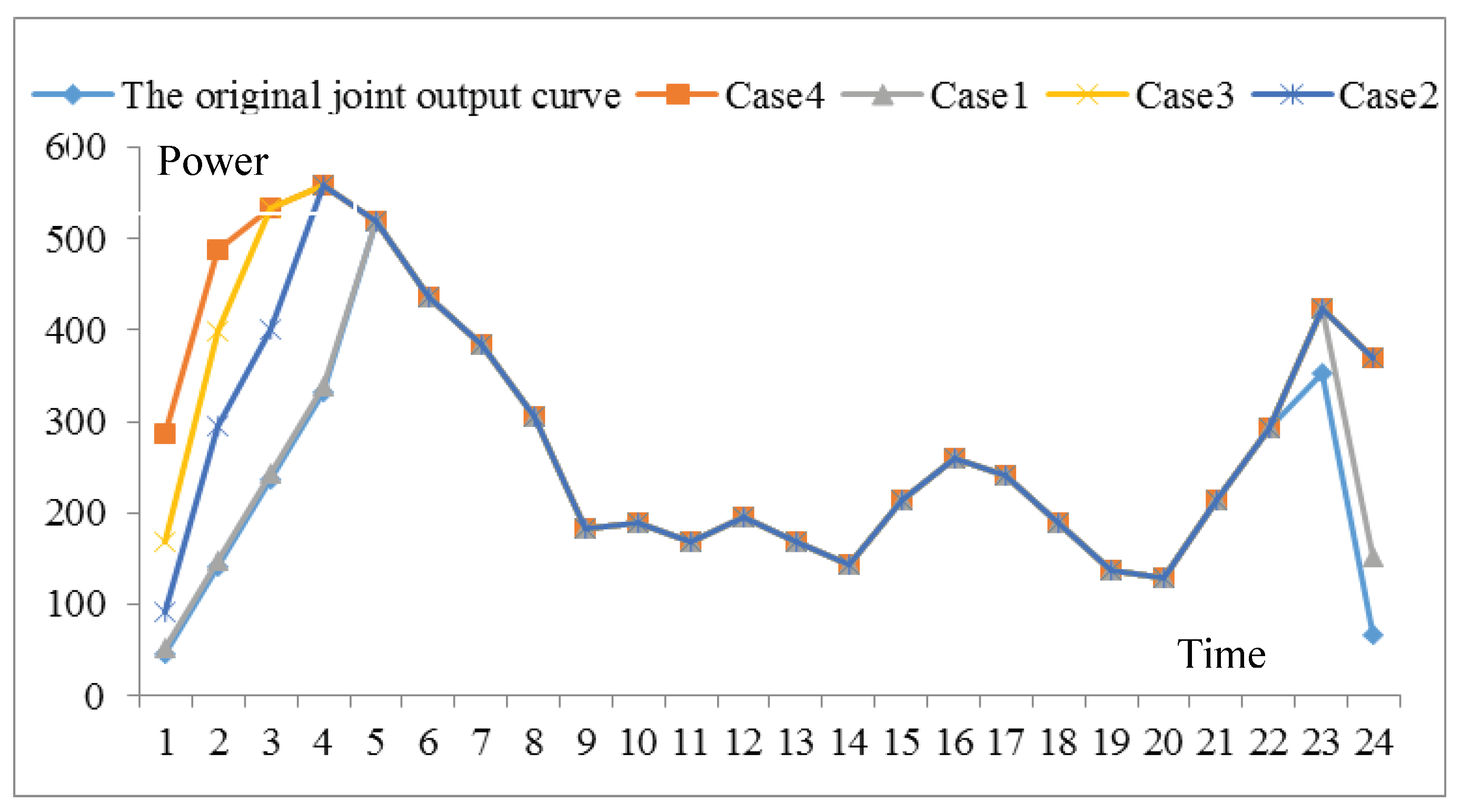
4.3. Case Analysis
4.4. Comparison of Four Scenarios
5. Conclusions
Author Contributions
Funding
Conflicts of Interest
References
- Bozchalui, M.C.; Hashmi, S.A.; Hassen, H.; Cañizares, C.A.; Bhattacharya, K. Optimal operation of residential energy hubs in smart grids. IEEE Trans. Smart Grid 2012, 3, 1755–1766. [Google Scholar] [CrossRef]
- Zhang, X.; Shahidehpour, M.; Alabdulwahab, A. Optimal Expansion Planning of Energy Hub with Multiple Energy infrastructures. IEEE Trans. Smart Grid 2015, 6, 2302–2311. [Google Scholar] [CrossRef]
- Lu, N.; Zhou, J.; He, Y. Particle swarm optimization-based neural network model for short-term load forecasting. Power Syst. Prot Control 2010, 38, 65–68. [Google Scholar]
- Sedghi, M.; Ahmadian, A.; Aliakbar-Golkar, M. Optimal Storage Planning in Active Distribution Network Considering Uncertainty of Wind Power Distributed Generation. IEEE Trans. Power Syst. 2015, 31, 304–316. [Google Scholar] [CrossRef]
- Abreu, L.V.L.; Khodayar, M.E.; Shahidehpour, M.; Wu, L. Risk-constrained coordination of cascaded hydro generators with variable wind power generation. IEEE Trans. Sustain. Energy 2012, 3, 359–368. [Google Scholar] [CrossRef]
- Xiang, X.; Song, Y.; Hu, Z.; Xu, Z. Research on optimal time of use price for electric vehicle participating V2G. Proc. CSEE 2013, 33, 15–26. [Google Scholar]
- Chen, H.; Xuan, P.; Wang, Y.; Tan, K.; Jin, X. Key technologies for integration of multi-type renewable energy sources: Research on multi-time frame robust scheduling dispatch. IEEE Trans. Smart Grid 2015, 7, 471–480. [Google Scholar] [CrossRef]
- Zou, Y.; Yang, L. Synergetic dispatch models of a wind/PV/hydro. Power Syst. Technol. 2015, 39, 1855–1860. [Google Scholar]
- Chen, J.; Wu, W.; Zhang, B. A robust interval wind power dispatch method considering the tradeoff between security and Economy. Proc. CSEE 2014, 34, 1033–1041. [Google Scholar]
- Coelho, V.N.; Coelho, I.M.; Coelho, B.N. Multi-objective BESS power dispatching using plug-in vehicles in a smart-micro grid. Renew. Energy 2016, 89, 730–742. [Google Scholar] [CrossRef]
- Wanc, L.; Sinch, C. Stochastic combined heat and power dispatch based on multi-objective particle swarm optimization. Int. J. Electr. Power Energy Syst. 2008, 30, 226–234. [Google Scholar] [CrossRef]
- Fan, S.; Ai, Q.; He, X. Risk analysis on dispatch of virtual power plant based on chance constrained programming. Proc. CSEE 2015, 39, 66–75. [Google Scholar]
- Liu, Z.; Wen, F.; Ledwich, G. Optimal siting and sizing of distributed generators in distribution systems considering uncertainties. IEEE Trans. Power Deliv. 2011, 26, 2541–2551. [Google Scholar] [CrossRef]
- Guandalini, G.; Campanari, S.; Romano, M.C. Power-to-gas plants and gas turbines for improved wind dispatchability: Energy and economic assessment. Appl. Energy 2015, 147, 117–130. [Google Scholar] [CrossRef]
- Dueñas, P.; Leung, T.; Gil, M.; Reneses, J. Gas-electricity coordination in competitive markets under: Renewable uncertainty. IEEE Trans. Power Syst. 2015, 30, 123–131. [Google Scholar] [CrossRef]
- Clegg, S.; Mancarella, P. Integrated modeling and assessment of the operational impact of power-to-gas(P2G) on electrical and gas transmission networks. IEEE Trans. Sustain. Energy 2016, 6, 1234–1244. [Google Scholar] [CrossRef]
- Correa-Posada, C.M.; Sanchez-Martin, P. Security-constrained optimal power and natural-gas flow. IEEE Trans. Power Syst. 2014, 29, 1780–1787. [Google Scholar] [CrossRef]
- Salimi, M.; Ghasemi, H.; Adelpour, M.; Vaez-ZAdeh, S. Optimal planning of energy hubs in interconnected energy systems: A case study for natural gas and electricity. IET Gener. Transm. Distrib. 2015, 9, 695–707. [Google Scholar] [CrossRef]
- Ntomaris, A.V.; Bakirtzis, A.G. Stochastic scheduling ofhybrid power stations in insular power systems with high wind penetration. IEEE Trans. Power Syst. 2016, 31, 3424–3436. [Google Scholar] [CrossRef]
- Hozouri, M.A.; Abbaspour, A.; Fotuhi-Firuzabad, M.; Moeini-Aghtaie, M. On the use of pumped storage for wind energy maximization in transmission-constrained power systems. IEEE Trans. Power Syst. 2015, 30, 1017–1025. [Google Scholar] [CrossRef]
- Wenlue, D.; Qun, W.; Li, Y. A coordinated dispatching model for a distribution utility and virtual power plants with wind/photovoltaic/hydro generators. Autom. Electr. Power Syst. 2015, 39, 75–81. [Google Scholar]
- Mohammadi, J.; Rahimi-kian, A. Aggregated wind power and flexible load offering strategy. IET Renew. Power Gener. 2007, 5, 439–447. [Google Scholar] [CrossRef]
- Pandzic, H.; Kuzle, I. Virtual power plant mid-term dispatch optimization. Appl. Energy 2013, 101, 134–141. [Google Scholar] [CrossRef]
- Sun, Y.; Wu, J.; Li, G.; He, J. Dynamic economic dispatch considering wind power penetration based on wind speed forecasting and stochastic programming. Proc. CSEE 2009, 29, 41–47. [Google Scholar]
- Wei, L.; Zhao, B.; Wu, H. Optimal allocation model of BESS system in virtual power plant environment with a high penetration of distributed photovoltaic generation. Autom. Electr. Power Syst. 2015, 39, 66–74. [Google Scholar]
- Carrion, M.; Arroyo, J.M. A computationally efficient mixed-integer linear formulation for the thermal unit commitment problem. IEEE Trans. Power Syst. 2006, 21, 1371–1378. [Google Scholar] [CrossRef]
- Zhang, W.; Wang, X.; Wu, X.; Yao, L. An analysis model of power system with large-scale wind power and transaction mode of direct power purchase by large consumers involved in system scheduling. Proc. CSEE 2015, 35, 2927–2995. [Google Scholar]


| Climbing Rate | ||||||||||||
|---|---|---|---|---|---|---|---|---|---|---|---|---|
| #1 | 100 | 18 | 0.04 | 6.4 | 0.4276 | 1 | 0.0032 | 100 | 600 | 3.02 × 10⁻⁵ | 0.822 | 22.8 |
| #2 | 200 | 10 | 0.05 | 8.6 | 0.03579 | 1 | 0.0034 | 100 | 650 | 2.95× 10⁻⁵ | 0.824 | 23.5 |
| #3 | 200 | 17 | 0.04 | 9.8 | 0.0248 | 1 | 0.0021 | 250 | 800 | 3.21× 10⁻⁵ | 0.830 | 24.1 |
| #4 | 100 | 15 | 0.1 | 4.2 | 0.01153 | 1 | 0.002 | 300 | 1000 | 4.65× 10⁻⁵ | 0.843 | 22.7 |
| #5 | 200 | 20 | 0.05 | 10.2 | 0.5276 | 1 | 0.0035 | 100 | 250 | 6.17× 10⁻⁵ | 0.861 | 19.3 |
| #6 | 220 | 22 | 0.05 | 10.8 | 0. 6276 | 1 | 0.0038 | 100 | 150 | 8.79× 10⁻⁵ | 0.833 | 15.3 |
| Period | Valley Period | Normal Period | Peak Period |
|---|---|---|---|
| Time | 0:00–5:00; 21:00–24:00 | 5:00–8:00; 14:00–19:00 | 8:00–14:00; 19:00–21:00 |
| Case | System Load Structure (%) | System Load | Wind and Photovoltaic Power | Thermal Power | ||||
|---|---|---|---|---|---|---|---|---|
| Valley Period | Normal Period | Peak Period | Maximum Load (MW) | Minimum Load (MW) | Grid Connected Power (MWh) | Grid Connected Power (MWh) | Coal Consumption (g/kW) | |
| Case1 | 25.3 | 33.2 | 41.5 | 2700 | 900 | 8432 | 36,468 | 328.6 |
| Case2 | 25.5 | 33.3 | 41.2 | 2620 | 950 | 8561 | 36,339 | 327.5 |
| Case3 | 27.3 | 33.9 | 38.8 | 2350 | 900 | 8666 | 30,894 | 325.4 |
| Case4 | 27.4 | 34 | 38.5 | 2220 | 980 | 8983 | 30,357 | 323.9 |
| Generator | Case 1 | Case 2 | Case 3 | Case 4 |
|---|---|---|---|---|
| 1# | 14,400 | 14,400 | 14,400 | 14,400 |
| 2# | 8571 | 8908 | 7526 | 7326 |
| 3# | 6449 | 6835 | 5217 | 5017 |
| 4# | 3312 | 3772 | 3032 | 2938 |
| 5# | 2800 | 2341 | 680 | 677 |
| 6# | 812 | 0 | 0 | 0 |
| Case | Valley Period | Normal Period | Peak Period | |||
|---|---|---|---|---|---|---|
| Charging | Discharging | Charging | Discharging | Charging | Discharging | |
| Case 2 | 160 | × | 124.2 | × | × | 270 |
| Case 4 | 198.6 | 18.3 | 157.2 | 40 | × | 261.2 |
© 2019 by the authors. Licensee MDPI, Basel, Switzerland. This article is an open access article distributed under the terms and conditions of the Creative Commons Attribution (CC BY) license (http://creativecommons.org/licenses/by/4.0/).
Share and Cite
Wang, G.; Tan, Z.; Tan, Q.; Yang, S.; Lin, H.; Ji, X.; Gejirifu, D.; Song, X. Multi-Objective Robust Scheduling Optimization Model of Wind, Photovoltaic Power, and BESS Based on the Pareto Principle. Sustainability 2019, 11, 305. https://doi.org/10.3390/su11020305
Wang G, Tan Z, Tan Q, Yang S, Lin H, Ji X, Gejirifu D, Song X. Multi-Objective Robust Scheduling Optimization Model of Wind, Photovoltaic Power, and BESS Based on the Pareto Principle. Sustainability. 2019; 11(2):305. https://doi.org/10.3390/su11020305
Chicago/Turabian StyleWang, Guan, Zhongfu Tan, Qingkun Tan, Shenbo Yang, Hongyu Lin, Xionghua Ji, De Gejirifu, and Xueying Song. 2019. "Multi-Objective Robust Scheduling Optimization Model of Wind, Photovoltaic Power, and BESS Based on the Pareto Principle" Sustainability 11, no. 2: 305. https://doi.org/10.3390/su11020305