Combinational Scheduling Model Considering Multiple Vehicle Sizes

Abstract

Urban public transport is an effective way to solve urban traffic problems and promote sustainable development of urban traffic. A scientific operation scheduling system has an important guiding significance for optimizing the configuration of urban public transport capacity resources, improving the level of operation organization and management, and providing for the sustainability of the transportation system. According to the inhomogeneous distribution of passenger flow along transit lines, this study develops a combinational scheduling model in which the enterprise supplies zonal service based on regular service. The objective function minimizes the sum of passenger travel cost and operation cost, and the simulated annealing algorithm is designed to solve the optimization model. This paper abstracts an ideal example by taking a real-world case of Bus Line 131 in Lanzhou, China. The numerical example is used to verify the validity of the model and algorithm. Results show that the combinational operation scheme can effectively satisfy passengers’ demand and reduce the total cost by 7.03% in comparison with the regular operation system. The optimal combinational system with the lowest total cost can increase the vehicle load factor and improve the utilization ratio.

1. Introduction

Recently, the scale of cities has continued to expand in China, and the living space of residents has become widely dispersed, resulting in increasing spatial imbalance in passenger travel. Conventional public transit plays an important role in urban public transportation. For passenger flow corridors with uneven distribution of passenger flow along the line, the traditional single dispatching mode results in higher load rate and overcrowded passengers in the maximal section of passenger flow. By contrast, the problem of lower load rate and wasted transport capacity occurs in the minimal section of passenger flow. Therefore, the combined scheduling mode of zonal vehicles must be studied to improve the match between passenger flow and transport capacity according to the spatial distribution characteristics of passenger flow along the line.

The major contributions of this paper can be summarized into the following ingredients:

*

On the basis of the practical project of Bus Network Operation Planning in Lanzhou (capital of Gansu Province, China), this study abstracts an ideal example by taking Bus Line 131 as the background, develops a optimal model of combined scheduling, and designs a simulated annealing algorithm to solve the problem. It provides a theoretical basis and method reference for optimizing the allocation of transportation resources and the organization of passenger transport for the department of bus operation and management.

*

The results of the study are consistent with the investigation and analytical report of our project group, thus validating the scientific nature and applicability of the model as well as the accuracy and effectiveness of the established parameters.

*

The results show that the combined operation scheduling scheme can better match the transport capacity and the demand of passenger flow. Under the same demand of passenger flow, the total cost of the combined scheduling scheme is lower than that of a single scheduling mode. An optimal combinational scheme minimizes the total cost of the system, increases the full load ratio, and improves the utilization rate of vehicles. It is of great practical significance to guide the operation planning of bus network.

2. Literature Review

Scholars have made great achievements in the optimization of combined scheduling mode for buses. Ceder studied the bus dispatch strategy of the main station express bus and interval bus. The timetables were constructed using two key concepts: assigning capacity and shifting departure times. The implementation of a mixed fleet of different vehicle sizes showed to be a promising way for achieving both an even headway and an even loading [1]. Site and Filippi constructed an interzonal bus scheduling model using an enterprise operation subsidy by taking public transport radiation as the research object. Its application to a case representative of radial corridor conditions showed the effects on service patterns and the trade-offs over operation periods between users’ and operator’s costs, stemming from different design criteria according to the weights attached to these two roles [2]. Ming et al. constructed a combined scheduling bus model under three modes of full-length bus, zonal bus, and main station express bus to optimize the total time cost of the system. In comparison with the traditional bus modulation, the multi-modal bus combination led to fewer departures and thus a lower time cost for the whole system [3]. Hu et al. constructed an optimization model for the combined scheduling of urban zonal buses and full-length buses, and realized the operation scheme of zonal buses with a minimum fleet size. The result showed that the number of vehicles running the inter-zone line was optimized after combinational scheduling between inter-zone vehicles and regular vehicles [4]. Wu et al. constructed a combined scheduling model of zonal buses based on the goal of optimal total social benefits given the limitation of transportation capacity in actual operation. Using the model, the relationship of the frequency, location of short-turning, and cost was analyzed. The result indicated that the mixed scheduling could reduce system costs and travel time when compared with the single scheduling in the case of unbalanced passenger flow distribution and capacity limitation [5]. Yang et al. constructed the multi-objective optimization scheduling model of Bus Rapid Transit (BRT) given factors: multiple vehicle types and bus capacity. The problem was divided into two sub-problems: with and without a bus queue; an analytical method was put forward to find this multi-objective model’s Pareto solution set. Lanzhou BRT line was chosen for the dispatching optimization model and the results illustrate the effectiveness of the optimization model and algorithm [6]. Yang et al. established a combined scheduling optimization model of zonal buses and full-length buses in consideration of the congestion perception cost of passengers on the bus. An application of the models to the case showed that the optimizing models are practical and effective for satisfying the demands of passengers and improving the operating efficiency of bus transit system [7]. Xu et al. optimized train planning of full-length and short-turn routing in consideration of the equilibrium of load factor, which has certain guiding significance for a combinational scheduling model. The numerical example results indicated that the formation plan, i.e., “the full-length train takes more carriages while the short-turn train takes fewer”, could improve the equilibrium of load factor between full-length and short-turn trains [8].

Palma and Lindsey analyzed optimal timetables for a given number of public transport vehicles on a single transit line when ridership varies with respect to the times at which riders prefer to travel and the schedule delay costs they incur from traveling earlier or later than desired. This solution was compared with the optimal schedule for the “circle” model in which preferred travel times were uniformly distributed over a 24-h day and trips could be rescheduled between days [9]. Vijayaraghavan and Anantharamaiah discussed fleet assignment strategies in urban transportation using express and partial service. Under consideration were the conditions in which the saving of a few buses in the fleet was possible by inserting express and partial services in the schedule with alternative fleet assignment strategies [10]. Tirachini et al. developed a short turning model using demand information from stations within both a single bus line and single period setting, aimed at increasing the service frequency on the more loaded sections to confront the spatial concentration of demand considering both operators and users. Applications on actual transit corridors exhibiting different demand profiles were conducted, calculating the optimal values for the design variables and the resulting benefits for each case. Results showed the typical demand configurations that were better served using a short turn strategy [11]. Shrivastava and O’Mahony developed a model in which feeder routes and frequencies leading to schedule coordination of feeder buses with main transit were developed simultaneously using genetic algorithms. The coordinated schedules of feeder buses were determined for the existing given schedules of main transit. Thus the developed feeder routes and schedules were complementary to each other. The results of the proposed model indicated improved load factors on developed routes; the overall load factor was also improved considerably in comparison with the earlier model [12]. Adamski et al. supplied the simulation decision support tool for which the dynamic optimal dispatching control purposes were developed, with the use of the SIMULINK package with Toolboxes. The following optimal dispatching control problems were solved: (1) punctuality control, regularity control, and synchronizing control with linear feedback as well as system state constraints; (2) stochastic control with real-time estimation of the model parameters; and (3) bus route zone control for synchronizing passenger transfers or the operation of different lines on common segments of the route [13]. Kim et al. developed a bus headway control model that could monitor and assess punctuality of an operation. This model was based on real-time event data, such as bus stop departures and arrivals for buses operating on a line-based timetable that had been constructed for each bus stop [14].

Parbo et al. explored timetable optimization from the perspective of minimizing the waiting time experienced by passengers when transferring either to or from a bus. A heuristic solution approach was developed using the idea of varying and optimizing the offset of the bus lines [15]. Cristián et al. developed a model that combined short turning and deadheading in an integrated strategy for a single transit line in which the optimization variables were both of a continuous and discrete nature, i.e., frequencies within and outside the high demand zone, vehicle capacities, and those stations where the strategy began and ended. They found that the integrated strategy could be justified in many cases with mixed load patterns, where unbalances within and between directions were observed. In general, the short turning strategy might yield large benefits in terms of total cost reductions, while low benefits were associated with deadheading due to the extra cost of running empty vehicles in some sections [16]. Ceder formulated the public transport vehicle scheduling using a multiple-vehicle type problem as a cost-flow network problem with an NP-hard complexity level by developing a heuristic algorithm based on the Deficit Function theory [17]. Hassold et al. proposed a methodology for the multiple-vehicle type vehicle scheduling problem. The methodology was based on a minimum cost network flow model utilizing sets of Pareto-optimized timetables for individual bus lines. It was demonstrated that a substitution of vehicles was beneficial and could lead to significant cost reductions [18]. Eberlein et al. formulated the real-time deadheading problem in transit operations control, optimally solved a simplified version of the general formulation, and demonstrated that the solutions of the simpler problem were good approximations to the solutions of the more general problem [19]. Jara-Díaz et al. described and analyzed the evolution of microeconomic models for the analysis of public transport services with parametric demand, leading to a more comprehensive model. An extension of Jansson’s model for a single period was developed analytically, which included the effect of vehicle size on operating costs and the influence of crowding on the value of time [20]. Jara-Díaz et al. constructed microeconomic public transport models with aggregate and disaggregate demand. The theoretical analysis and the numerical examples suggested that the spatially aggregated model underestimates optimal frequency and overestimates vehicle size [21]. Leiva et al. designed limited-stop services for an urban bus corridor with capacity constraints, formulated various optimization models that could accommodate the operating characteristics of a bus corridor, given an origin–destination trip matrix and a set of services [22]. Ibarra-Rojas et al. presented two integer linear programming models for the timetabling and vehicle scheduling problems, and combined them in a bi-objective integrated model. This allowed for the analysis of the trade-off between level of service and operating costs of transit networks in terms of Pareto fronts [23]. Kim et al. proposed probabilistic optimization models, which confronted the stochastic variability in travel times and wait times and were formulated for integrating and coordinating bus transit services for one terminal and multiple local regions. Solutions for decision variables, which included the selected service type for particular regions, the vehicle size, the number of zones, headways, fleet, and slack times, were determined via analytic optimization or numerical methods. The proposed models generate either common headway or integer-ratio headway solutions for timed transfer coordination based on the given demand [24]. Wu et al. proposed a novel stochastic bus schedule coordination with demand assignment and passenger rerouting in case of transfer failure; additionally, a bi-level programming model in which the schedule design and passenger route choice were determined simultaneously via two travel strategies: non-adaptive and adaptive routings. Results showed that when the rerouting behavior was considered, a more cost-effective schedule coordination scheme with less excess time could be achieved; ignoring such an effect would underestimate the efficacy of schedule coordination scheme [25].

Li et al. proposed a robust dynamic control mechanism for the bus transit system, taking into account variations in congestion delays and passenger demand as well as combined bus holding and operating speed control strategies. By using a prespecified uncertainty set, they proposed a state space model for bus motion with delay disturbances and passenger demand uncertainties. According to the Lyapunov function analysis method, they designed a robust dynamic control based on the state-feedback scheme as the bus control to achieve robust stability of the bus transit system, which effectively reduced the bus bunching phenomenon. The problem was solved in a polynomial time and satisfied the practical real-time requirement [26]. Huang et al. studied the shortest path problems in electric transit bus scheduling and electric truck routing with time windows and developed a label-correcting algorithm with state space relaxation to find optimal solutions. The computational experiments resulted show that the label-correcting algorithm performed very well [27]. Han et al. confronted the problem of an aggregator coordinating charging schedules of electric vehicles with the objective of minimizing the total charging cost, using the assumption that the maximum charging power could vary according to the current state of charge. They proposed two charging plans: non-preemptive and preemptive charging. The difference between the two plans was whether interruptions during the charging process were allowed or not; they then formulated the electric vehicle charging-scheduling problem for each plan and proposed a formulation that could prevent frequent interruptions. They showed that the proposed formulations could be applied in practice to solve scheduling problems with regard to charging [28]. Chen et al. proposed the underlying scheduling problem with the primary objective of optimizing the total costs for both passengers and operating agencies, as well as with the secondary objective of minimizing bus emissions. The results showed that the proposed scheduling strategy outperformed the other operating strategy with respect to operational costs and bus emissions. A sensitivity study investigated the impact of the fleet size in operations and passenger demand on the effectiveness of the proposed stop-skipping strategy in consideration of bus emissions [29]. Chen et al. established a bus route headway allocation model by considering the influence of three uncertainties on the bus route headway: passenger demand elasticity, the randomness of bus travel time between bus stops, and the abandoned passengers flow. An enumeration combining a recursive algorithm under Monte Carlo random simulation conditions was designed to solve the problem. The results showed that the model could reduce the wait time of passengers and attract more passengers to travel by bus [30]. Bányai describes a real-time scheduling optimization model focusing on the energy efficiency of the operation and introduces a mathematical model of last mile delivery problems including scheduling and assignment problems. The objective of the model was to determine the optimal assignment and scheduling for each order to minimize energy consumption, allowing for improved energy efficiency. A black-hole optimization-based heuristic is described, whose performance is validated with different benchmark functions. The scenario analysis validates the model and evaluates its performance to increase energy efficiency in last mile logistics [31].

The aforementioned studies are significant in investigating the optimization of bus combined scheduling. However, most studies consider only the single scheduling mode of multiple vehicle models or the combined scheduling mode of the same vehicle model, and the combined scheduling mode of multiple vehicle models are rarely considered.

3. Combined Scheduling Optimization Problem

3.1. Basic Notation and General Assumptions

Given a bus line, the notation used throughout this paper is given in

Table 1. Summary of Notations.

Notation	Definitions and Units
$N_s$	total stations of a bus line
$d$	the running direction of buses, d = 1 is up direction, while d = 2 is down direction
$S_u$	the departure station of zonal bus
$S_v$	the turn-back(terminal) station of zonal bus
$h$	bus line, h = 1 denotes the full-length service line, and h = 2 the zonal service line
$f_h$	frequency of line $h$, buses/h
$f_m$	maximum frequency of bus line, buses/h
$f_p$	Policy frequency of bus line, i.e., minimum frequency depend on service level, buses/h
$c_w$	waiting time value, CNY/h
$c_t$	in-vehicle time value, CNY/h
$t_{r,k}$	the bus’s running time on the $k^{th}$ section, min
$t_{s,k}$	dwell time at the $k^{th}$ station, second
$c_{\mathrm{o}}^h$	depreciation cost per bus-hour on line $h$, CNY/bus-h
$c_r^h$	running cost per bus-kilometers of line $h$, CNY/bus-km
$T_{c1}$	the buses’ cycling time of full-length service line, min
$T_{c2}$	the buses’ cycling time of zonal service line, min
$L_h$	length of line h, km
$T$	time horizon of vehicle scheduling, h
$C_h$	bus capacity of line $h$, pass/bus
$R_h$	section set of line $h$
$Q_{h,r}$	section flow shared by the $r^{th}$ section of bus line $h$
${\lambda }_{ij}^1$,${\lambda }_{ij}^2$	the passenger volume per hour from station $i$ to station $j$ in up direction and down direction, respectively, pass/h
$\vartheta$	layover time at turn-back station, min
${\delta }_h$	maximum load rate of bus belonging to line h
${\delta }_m$	maximum load rate of the bus

.

3.2. Problem Description

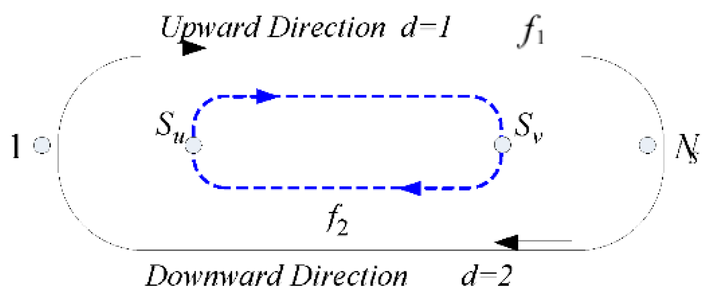
Figure 1 shows a bus line with a total of $N_s$ stations. The upward direction of bus operation is from station 1 to station $N_s$, which is denoted as d = 1. The reverse direction is the downward direction, which is denoted as d = 2. The conventional operation mode is the full-length service mode, that is, the bus departs from station 1 and runs until to reach station $N_s$, then turns back; we call this single-scheduling mode. In this operation, the bus can service all the passengers at any station. However, the zonal operation mode is that the bus departs from an intermediate station $S_u$, runs until to an intermediate station $S_v$ , and then returns. In the zonal operation mode, the buses can only service partial passengers boarding from the station $S_u$ to $S_v$. In real public transportation systems, we may often meet a situation in which passenger flow within the central city is much more than that in the suburbs; accordingly, the bus’s usage ratio is not equal between central city and suburb. According to this situation, the public transport enterprise will attempt to start the combinational scheduling mode, i.e., the conventional operation mode and zonal mode exist simultaneously in one line. Here, we denote the bus routing of conventional operation mode as full-length line, and that of zonal operation mode as zonal line, assuming the frequency of line h is $f_h$.

We develop a combinational scheduling model to minimum the total cost for a combinational scheduling mode, the decision variables of the minimization problem are $(S_u,S_v,f_1,f_2,C_1,C_2)$.

4. Combined Scheduling Model

The bus combined scheduling optimization model considers the travel time cost of passengers and the operation cost of enterprises. The travel time cost of passengers includes wait-time cost and on-board time cost. The operation cost of enterprises includes the vehicle loss cost and vehicle running cost.

4.1. Travel Cost of Passenger

The travel cost of the passengers includes wait-time cost and on-board time cost, in which wait time is related to departure interval. We assume that the bus arrives at the station in accordance with the Poisson distribution, and the passenger wait time is equal to the departure interval [9]. In the operations of zonal buses, the departure interval of the zonal bus coverage section ($S_u$ to $S_v$) is different from that of the peripheral section (1 to $S_u$ and $S_v$ to $N_s$) of zonal buses. The wait-time cost $C_1$ can be calculated as follows:

$$\begin{array}{l}{C}_1=\frac{c_w}{f_1}\left({\displaystyle \sum _{i=1}^{S_{\mathrm{u}}-1}{\displaystyle \sum _{j=i+1}^{N_s}{\lambda }_{ij}^1}}+{\displaystyle \sum _{i=S_v}^{N_s-1}{\displaystyle \sum _{j=i+1}^{N_s}{\lambda }_{ij}^1+{\displaystyle \sum _{i=S_u}^{S_v-1}{\displaystyle \sum _{j=S_v+1}^{N_s}{\lambda }_{ij}^1}}+{\displaystyle \sum _{i=S_v+1}^{N_s}{\displaystyle \sum _{j=1}^{i-1}{\lambda }_{ij}^2+{\displaystyle \sum _{i=2}^{S_u}{\displaystyle \sum _{j=1}^{i-1}{\lambda }_{ij}^2+{\displaystyle \sum _{i=S_u+1}^{S_v}{\displaystyle \sum _{j=1}^{S_u-1}{\lambda }_{ij}^2}}}}}}}}\right)\\ +\frac{c_w}{f_1+f_2}\left({\displaystyle \sum _{i=S_u}^{S_v-1}{\displaystyle \sum _{j=i+1}^{S_v}{\lambda }_{ij}^1}}+{\displaystyle \sum _{i=S_u+1}^{S_v}{\displaystyle \sum _{j=S_u}^{i-1}{\lambda }_{ij}^2}}\right)\end{array}$$

(1)

in which the first item represents the wait-time cost of passengers served by a full-length bus, and the second is wait-time cost of passengers boarding the bus between the station $S_u$ and $S_v$ and who are both served by full-length and short-turn bus.

The in-vehicle time cost of passengers $C_2$ can be expressed as follows:

$$C_2=c_t\left({\displaystyle \sum _{i=1}^{N_s-1}{\displaystyle \sum _{j=i+1}^{N_s}{\displaystyle \sum _{k=i}^{j-1}{t}_{r,k}{\lambda }_{ij}^1}}}+{\displaystyle \sum _{i=2}^{N_s}{\displaystyle \sum _{j=1}^{i-1}{\displaystyle \sum _{k=j}^{i-1}{t}_{r,k}{\lambda }_{ij}^2}}}\right)+c_t\left({\displaystyle \sum _{i=1}^{N_s-2}{\displaystyle \sum _{j=i+2}^{N_s}{\displaystyle \sum _{k=i+1}^{j-1}{t}_{s,k}{\lambda }_{ij}^1}}}+{\displaystyle \sum _{i=3}^{N_s}{\displaystyle \sum _{j=1}^{i-2}{\displaystyle \sum _{k=j+1}^{i-1}{t}_{s,k}{\lambda }_{ij}^2}}}\right)$$

(2)

where the first item represents total in-vehicle time cost that passengers spend on sections, and the second is the time passengers spend at stations.

4.2. Operation Cost of Enterprise

The operation cost of enterprise includes usage and operation costs of the vehicle. Usage costs refer to wear and depreciation cost of the vehicle. Operation costs refer to fuel expenses and wage expenses in operation. The total operating cost can be expressed as

$$C_3={\displaystyle \sum _{h=1,2}\left(c_o^h{f}_h{T}_{ch}^{}+2c_r^h{f}_h{L}_{h}T\right)}$$

(3)

$$T_{c1}=\vartheta +{\displaystyle \sum _{k=1}^{N_s-1}{t}_{r,k}+{\displaystyle \sum _{k=1}^{N_{\mathrm{s}}}{t}_{s,k}}}$$

(4)

$$T_{c2}=\vartheta +{\displaystyle \sum _{k=S_u}^{S_v-1}{t}_{r,k}+{\displaystyle \sum _{k=S_u}^{S_v}{t}_{s,k}}}$$

(5)

where Expressions (4) and (5) represent cycling times of full-length and zonal bus, respectively. The depreciation cost per bus-hour, $c_o^h$, is approximately equal to the ratio of bus’s acquisition cost to its working life. The cycling time includes three parts: the layover time at departure station and terminal, the running time on sections, and total dwell time at stations.

4.3. Model Construction

An optimal scheduling model is established to minimize the sum of operating costs and passenger travel costs.

$$\min Z=C_1+C_2+C_3$$

(6)

$$s.t.{\displaystyle \sum f_h}\le f_{m}h=1,2$$

(7)

$${\delta }_h\le {\delta }_{m}h=1,2$$

(8)

$$1\le S_u<S_v\le N_s$$

(9)

$$f_h=\underset{r\in R_h}{\max }\left(Q_{h,r}/C_h{\delta }_m\right)h=1,2$$

(10)

Formula (6) is the objective function. Formula (7) is the maximum frequency constraint of the bus, which considers the departure interval is not infinite. Formula (8) is the constraint of maximum full-load rate. Formula (9) is the operation range constraint of zonal bus, which keeps the zonal bus runs between station $S_u$ and $S_v$. Formula (10) is minimum frequency of line $h$ in operation period required by capacity constraint, whose detailed calculation method is presented in references [2,8].

5. Example Study

5.1. Solving Method

The solution idea of the model in this study is as follows: penalty function method is adopted to transform the constraint model into an unconstrained model, and the simulated annealing algorithm (SA) is designed to solve the unconstrained optimization model [2,8]. The SA have been successfully applied to solve the scheduling optimization problem [32,33], and the detailed process of SA is as follows.

5.1.1. Critical Steps in Design of Simulated Annealing Algorithm

1. Solution of encoding form and generating a new solution

Simulated annealing algorithm has probabilistic global optimization performance and has been widely used in the field of transportation planning. We chose it because several simulation experiments show that simulated annealing algorithm can produce a satisfactory approximate optimal solution when solving traffic optimization problems; additionally, the computation time is not very long.

The model of this paper has six decision variables, namely, $C_1$ (capacity of full-length buses), $C_2$ (capacity of zonal bus), $f_1$ (frequency of full-length bus), $f_2$ (frequency of zonal bus), $S_u$ (departure station of zonal bus), and $S_v$ (terminal of zonal bus). Accordingly, the encoding form of the solution can be expressed as $D_{var}=$ ($C_1$,$C_2$,$f_1$,$f_2$,$S_u$,$S_v$). If one assumes the first two decision variables are continuous while the last four are discrete, this leads to a difficult problem. To reduce the solving difficulty, we assume the bus capacity is discrete; this is a realistic assumption because the bus’s maximum capacity was fixed when the bus was produced. For example, in an area such as Lanzhou, a western city of China, the city has two types of buses and their maximum capacities are 60 and 90 passengers per bus.

To facilitate the solution, given an array $C$ = [60, 90], and convert the $C_1$ and $C_2$ into $C_1^{\prime }$ and $C_2^{\prime }$ (subscripts of the array C), respectively. 1 ≤ $C_1^{\prime }$ ≤ 2, 1 ≤ $C_2^{\prime }$ ≤ 2. When the subscript $C_1^{\prime }$ = 1 or $C_2^{\prime }$ = 1, the bus capacity is 60 people. When the subscript $C_1^{\prime }$ = 2 or $C_2^{\prime }$ = 2, the bus capacity is 90 people. The purpose of the transformation is convenient to generate a new solution in SA. Therefore, the encoding form of the solution can be expressed as $D_{var}^{\prime }=$($C_1^{\prime }$,$C_2^{\prime }$,$f_1$,$f_2$,$S_u$,$S_v$).

2. Generation of new solutions

In the simulated annealing algorithm, the generation of the new solution requires the random perturbation $\Delta x$ of the current solution $X_{opt}$. According to the coding form of the solution, the random perturbation $\Delta x$ is expressed as follows: the $i^{th}$ decision variable is randomly selected from M decision variables, and the perturbation direction of the decision variable is determined by probability $P_m$. The specific method is as follows:

Step 1: Select the decision variable. A random number $\kappa$ is generated, where $\kappa \in (0,1)$. $i=1+\lfloor \kappa \cdot M\rfloor$, and $\lfloor \rfloor$ indicates the round down.

Step 2: Determine random disturbance. A random number $\omega$ is generated, where $\omega \in \left(0,1\right]$. If $\omega <P_m$. Add 1 to the $i^{th}$ decision variable; otherwise, minus 1 from the $i^{th}$ decision.

Step 3: Judge whether the new solution is feasible. If the new solution is feasible, then stop the calculation; otherwise, return to Step 2.

5.1.2. Process of Simulated Annealing Algorithm

Step 1: Initialization. Set current temperature $T_c$, termination temperature $T_t$, and attenuation parameter of temperature $\alpha$. The initial feasible solution $X_0$ is generated randomly. The optimal solution $X_{opt}$ is obtained ($X_{opt}=X_0$). The value of the objective function $f(X_{opt})$ is calculated according to Equation (6).

Step 2: Generate new solution. According to the method of new solution generation, random disturbance is conducted on the current optimal solution $X_{opt}$. $X_{opt}^{\prime }=X_{opt}+\Delta x$. The objective function value of the new solution $f(X_{opt}^{\prime })$ and the increment of the objective function value $\Delta f=f(X_{opt}^{\prime })-f(X_{opt})$ are calculated.

Step 3: Given the acceptance probability $P$, if $\Delta f<0$, then the new solution is accepted as the current optimal solution, $X_{opt}=X_{opt}^{\prime }$. If $\Delta f\ge 0$, then the random number $\sigma$ is generated, $\sigma \in (0,1]$. If $\exp (-\Delta f/T_c)<\sigma$, then $X_{opt}=X_{opt}^{\prime }$; otherwise, the new solution is abandoned.

Step 4: Update the current temperature. If $T_c=\alpha \cdot T_c$, if $T_c>T_t$, then return to Step 2; otherwise, return to Step 3.

Step 5: End the calculation. The optimal solution $X_{opt}$ and objective function value $f(X_{opt})$ are output.

5.2. Example and Model Parameters

On the basis of the practical project of Bus Network Operation Planning in Lanzhou (capital of Gansu Province, China), we abstract an ideal example by taking Bus Line 131 as the background. For example, the total length of the line is 27 km with 28 stations in total; the distance between adjacent stations $l_r$ = 1 km. The departure station and terminal of the zonal buses are the 5th and 22nd stations, respectively. The running time between two adjacent stations is 2 min, and the dwell time is 20 s. The minimum frequency of full-length buses $f_p$ = 5 buses/h, and the maximum frequency of the bus line $f_m$ = 70 buses/h. Buses are divided into three types according to carrying capacity, namely, 60, 90, and 120 pass/bus. On the basis of field investigation within the Lanzhou Public Transport Company, the acquisition costs of three types of buses are 0.9 billion CNY, 1.1 billion CNY, 1.3 billion CNY respectively. The working life of all types of buses is 10 years and the service time is 12 h a day and 365 days per year; accordingly, the depreciation cost is about equal to 0.9/(10*365*12) = 20.54 CNY/h, 1.1/(10*365*12) = 25.1 CNY/h, 1.3/(10*365*12) = 29.7 CNY/h. On the basis of these variables, the fixed depreciation fee per bus-hour is set to 20, 25, and 30 CNY/h, respectively, and the running costs are 10, 16, and 22 CNY/(bus-km), respectively.

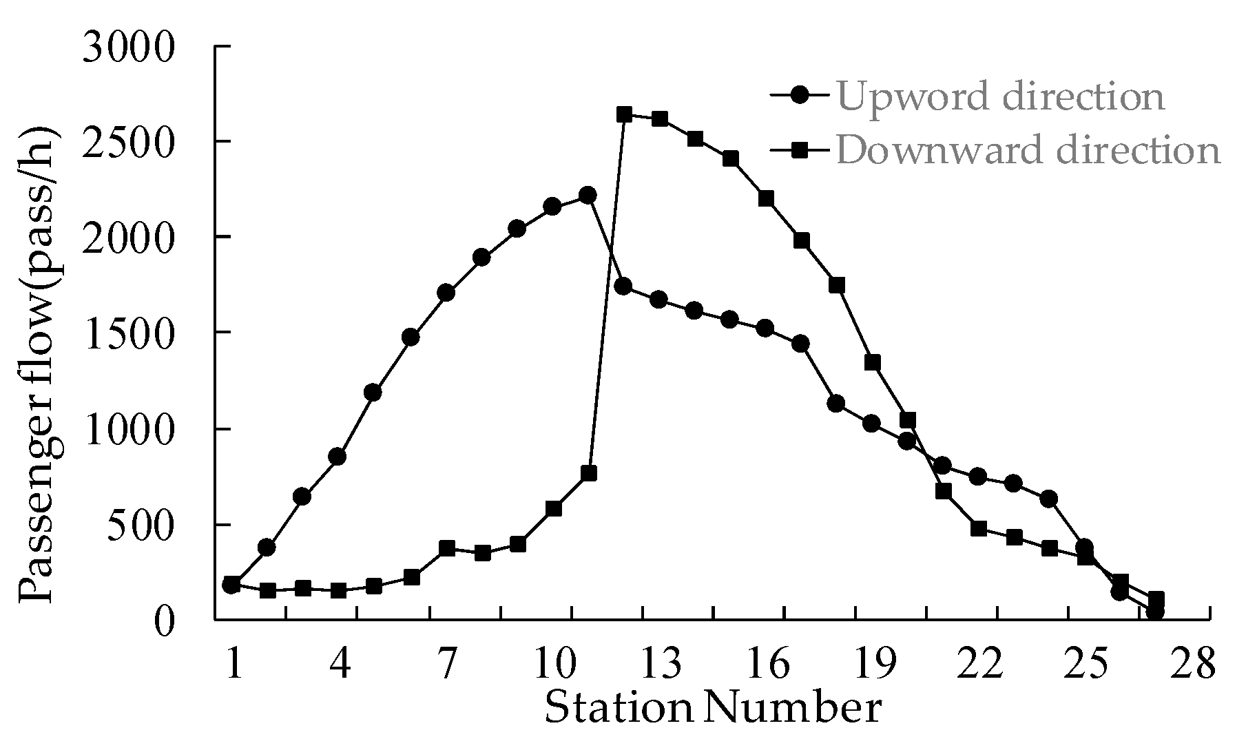
On the basis of Ref. [34], the average hourly wage in Lanzhou is 20 CNY/h. Taking into account that the passengers’ perception of time value for travelling is less than that for waiting, the passengers’ waiting time value is set to 25 CNY/h, and travelling time value is set to 20 CNY/h. The maximum load rate of the bus ${\delta }_m=0.9$. The current temperature of the simulated annealing algorithm $T_c$ = 100, the termination temperature $T_t$ = 10⁻⁴, the attenuation parameter of temperature $\alpha$ = 0.99, and the random disturbance probability $P_m=0.5$. The load profile of the Bus Line 131 in peak hour (7:30–8:30) is shown in Figure 2.

5.3. Result Analysis

The optimization results of the operation scheme in the morning peak time are shown in

Table 2. Comparison of Operation Schemes and Results during Morning Peak Time.

Operational Indicators	Single Scheduling Mode	Uniform Combinational Scheduling	Rate of Change (%)
		Full-Length Bus/Zonal Bus
Departure Station/Terminal of Zonal Bus	-	(5, 22)	-
Capacity of Bus(pass/bus)	90	90/60	-
Configuration Number of Bus(buses)	91	38/41	−13.19
Departure Frequency (buses/h)	33	15/27	+27.27
Operation Cost (104 CNY)	2.51	1.95	−22.31
Travelling Cost (104 CNY)	4.75	4.80	+1.05
Total Cost (104 CNY)	7.26	6.75	−7.03

with the single scheduling mode for comparison. The frequency is 33 buses/h, and the total cost is 72,600 CNY if the bus type (with carrying capacity of 90 pass/bus) is adopted under the single scheduling mode to meet the demand of passenger flow in the morning peak time.

Under the condition of adopting the mode of running zonal buses, 15 full-length buses and 27 zonal buses are placed into operation, and the total cost is 67,500 CNY. Although the travel cost of the passenger increased by 1.05%, the operating cost decreased by 22.31%. The total cost is 7.03% lower than that of single scheduling mode, indicating that the zonal bus operation can reduce the total cost of the system.

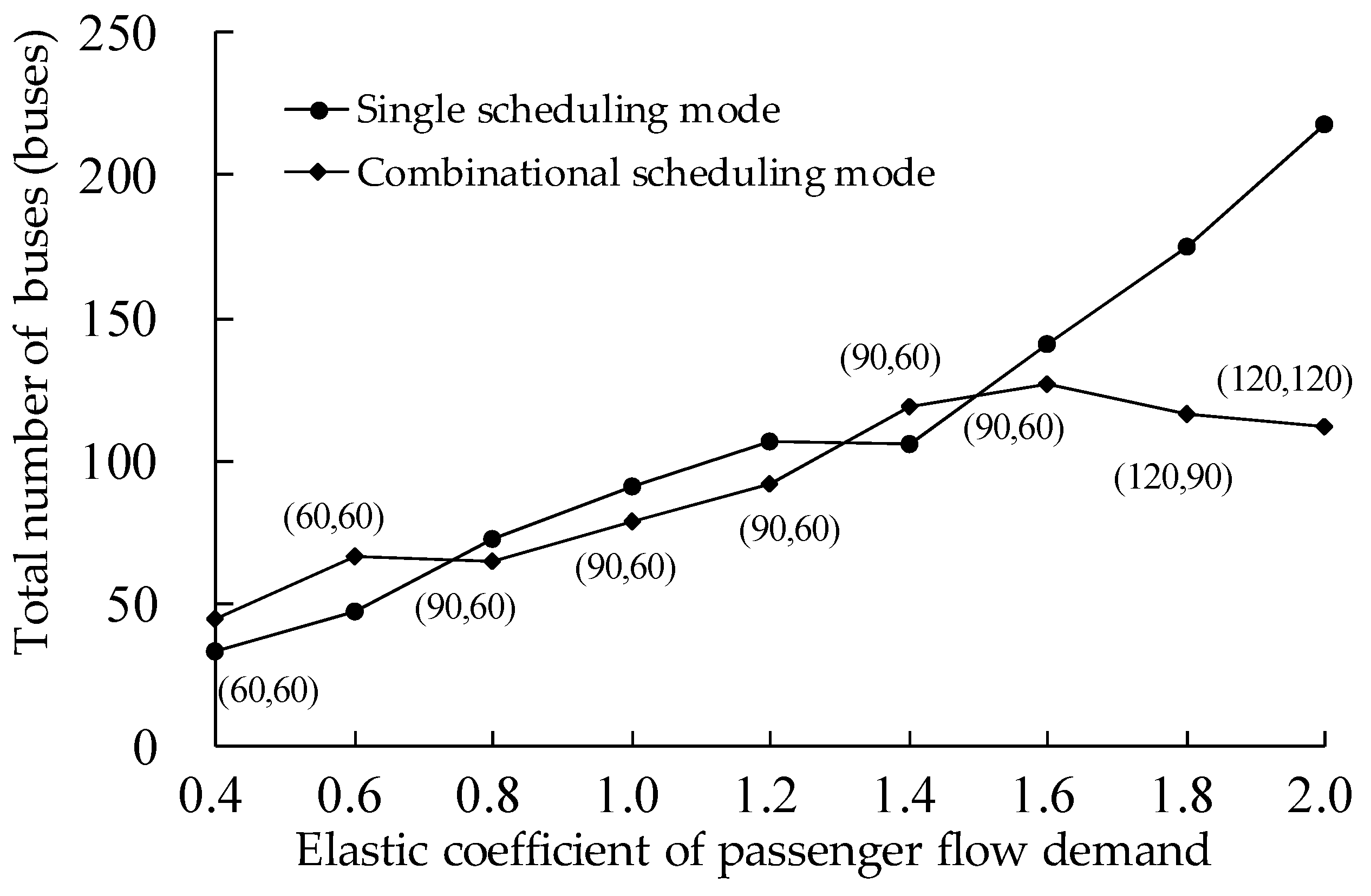
To analyze the effect of passenger demand changes on the operation plan, an elasticity coefficient of passenger flow demand is set, the OD matrix of the original passenger flow is multiplied by the elasticity coefficient to obtain different passenger requirements. The change trend of bus configuration quantity in the optimal operation scheme is studied under single scheduling (bus capacity: 90 pass/bus) and combined scheduling for different passenger flow demands. The results are presented in Figure 3 (the numbers in brackets represent carrying capacity of the bus under the combined scheduling mode). With the increase of passenger demand, the total number of buses in the single scheduling mode show an upward trend, whereas the total number of bus configurations under the combined scheduling mode show an initial increasing trend and then decreases gradually. When the passenger flow demand elasticity coefficient is greater than 1.6, the number of bus configurations under combined scheduling gradually decreases due to the increase in bus carrying capacity.

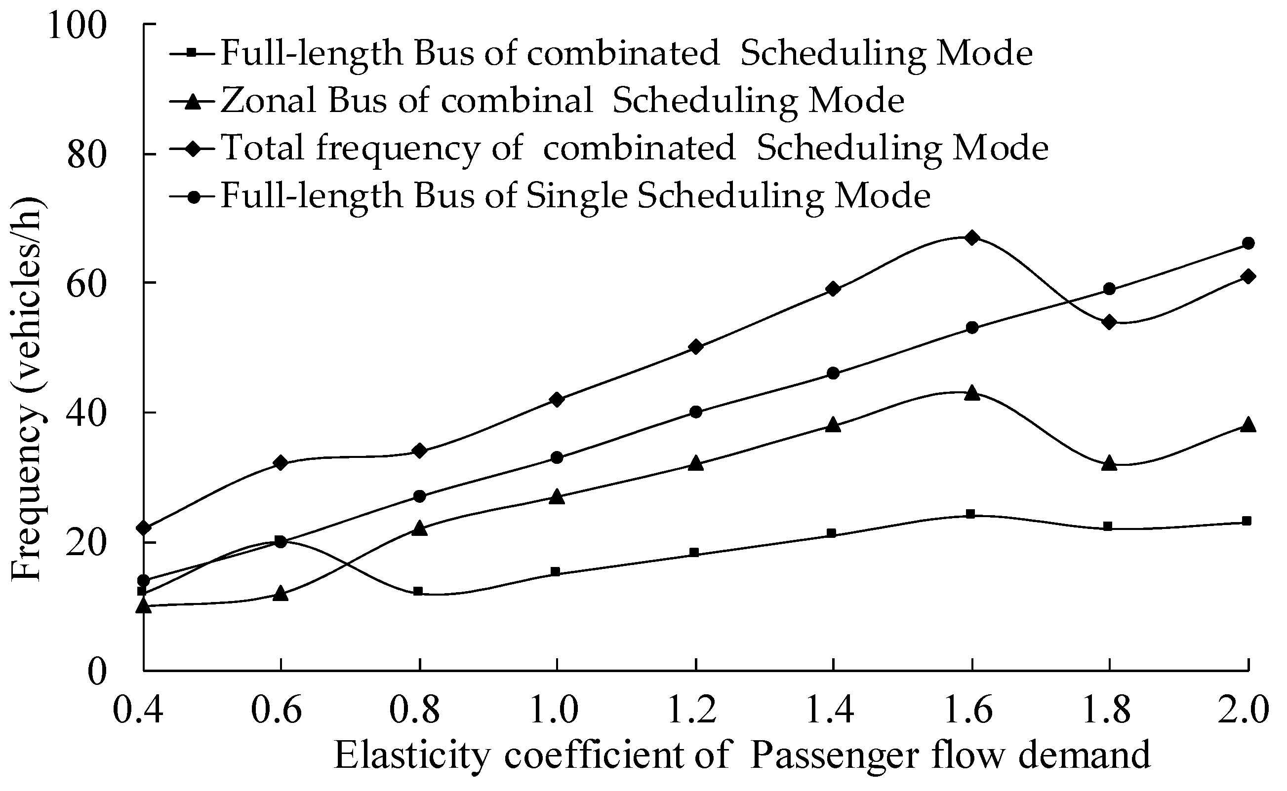
The variation of departure frequency under different passenger flow demands is shown in Figure 4. With the increase of passenger demand, the departure frequency of the single scheduling mode shows an upward trend, whereas the departure frequency under combined scheduling mode shows an initial increasing trend but then decreases. When the passenger flow demand elasticity coefficient is greater than 1.6, the departure frequency of combined scheduling fluctuates due to the change of bus carrying capacity.

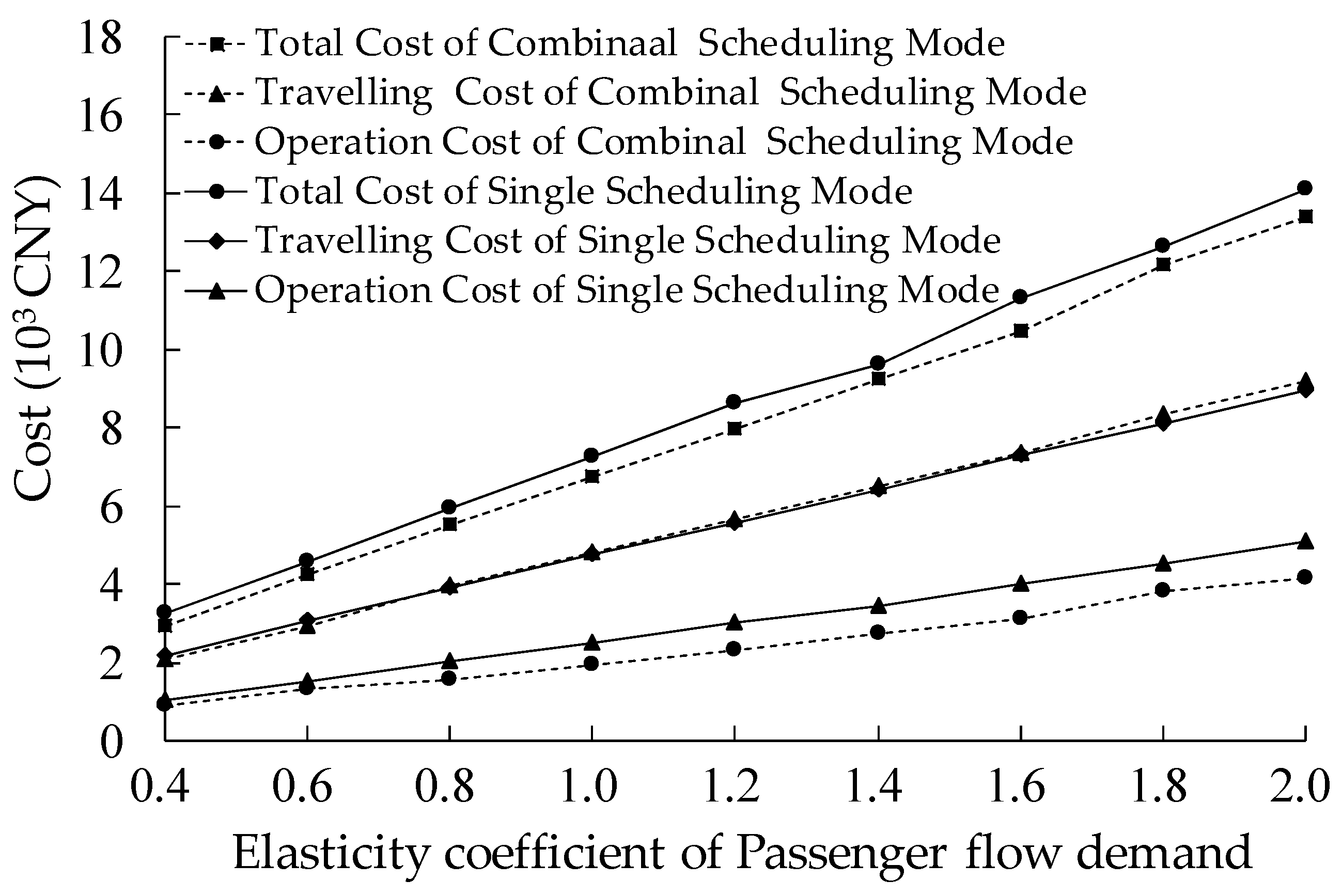
Under different passenger flow requirements, the cost changes of combined scheduling and single scheduling are shown in Figure 5. With the increase of passenger flow demand, the total cost of the system and the operating cost of the enterprise under combined scheduling are lower than the cost of single scheduling; however, the travel cost shows an initial lower trend but then becomes higher. The main reason ascribed to these trends is that when the passenger flow is small, the increase of waiting cost of peripheral passengers of zonal bus under combined scheduling is lower than the decreased waiting cost of passengers within the range of zonal bus. When the passenger flow is large, the increase of passenger waiting cost in the peripheral area is higher than the decreased passenger waiting cost within the range of the zonal bus.

The optimal operation scheme is obtained by fixing the departure and terminal stations as well as changing the bus type combination under combined scheduling. The results, in comparison with those of the single scheduling operation scheme, are shown in

Table 3. Comparison of Optimal Operation Schemes and Indicators under Different Bus Types.

Operation Indicators	Origin Station/Destination Station	Capacity of Bus (Pass/Bus)	Departure Frequency (Buses/h)	Bus Number (Buses)	Operation Cost (103 CNY)	Travel Cost (103 CNY)	Total Cost (103 CNY)	Change Rate of Operation Cost (%)	Change Rate of Travel Cost (%)	Change Rate of Total Cost (%)
		Full-Length Bus/Zonal Bus
Single Scheduling	-	90	33	91	2.51	4.75	7.26	-	-	-
Combined Scheduling	(5, 22)	90/60	15/27	38/41	1.95	4.80	6.75	−22.31	+1.05	−7.03
		120/60	10/32	24/48	1.99	4.93	6.92	−20.72	+3.79	−4.68
		120/90	13/16	31/25	2.09	4.99	7.08	−16.73	+5.05	−2.48

. Under different bus type combinations, operating costs of combined scheduling are all reduced, passenger travel costs are all increased, and total system costs are all reduced. Under the bus type combination of (90, 60), (120, 60), and (120, 90) pass/bus, the total cost is reduced by 7.03%, 4.68%, and 2.48%, respectively. The bus type combination of (90, 60) pass/bus is the optimal scheme. An optimal bus type combination scheme minimizes the total cost of the system.

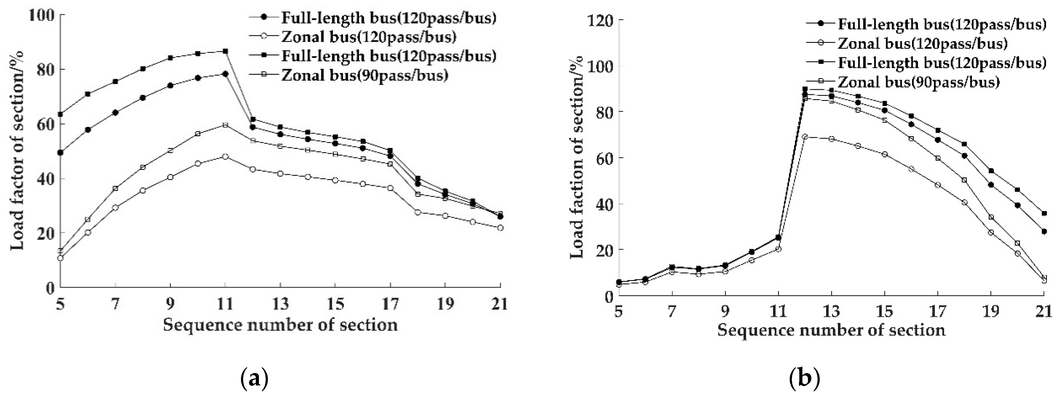
To study the service level of different bus type combination schemes, the section load rate under the bus type combination of (120, 120) and (120, 90) pass/bus is compared and analyzed, and the results are shown in Figure 6. Under the multi-type operation scheme, the bus load rate improves. According to this calculation, under the combined scheme of (120, 120) pass/bus, the average full-load rates of the full-length bus and the zonal bus in the upward direction are 44.17% and 31.52%, respectively. Under the combined scheme of (120, 90) pass/bus, the average load rates are 59.74% and 41.51%, respectively, which increased by 15.57% and 9.99%, respectively. Similarly, the average full load rate of the full-length bus and the zonal bus in the downward direction increases from 44.17% and 31.52 to 48.86% and 39.13%, respectively, which increases by 4.69% and 7.61%, respectively. The results show that the combined scheduling scheme of multiple bus types can increase the bus load rate and improve the bus utilization rate under the condition of meeting the service level.

6. Conclusions

Using an abstracted ideal example of Bus Line 131 of Lanzhou as the background and considering the mixed running situation of multiple bus types, this study established the optimal scheduling model of zonal buses; the solution method based on simulated annealing algorithm was proposed. The following conclusions are drawn:

(1)

In the combined dispatching mode of zonal buses running, the total cost of the system was 7.03% lower than that of the single dispatching mode, indicating that zonal buses running could reduce the total cost of system operation.

(2)

With the increase of passenger flow demand, the number of bus configurations, departure frequency, and various costs under a single scheduling mode all increased monotonically. However, under the combined dispatching mode, the number of bus configurations and departure frequency show an initial increasing but then decreasing tendency.

(3)

The optimal operation scheme under different bus types shows an optimal combination scheme of bus types, which minimizes the total cost of the system. Given the combined scheduling scheme of multiple bus types, the full-load rate of buses can be increased, and the utilization rate can be improved under the condition of meeting the service level.

We developed an optimal model of combinational scheduling mode but without taking into account factors such as transferring. In real-life situations, partial passengers who choose zonal buses and have a destination far away from the zonal bus’s terminal, have to alight on zonal bus’s terminal and then take the full-length bus to their destinations. Additionally, the passengers’ choosing behavior on common line sections is ignored. These disadvantages will be studied in future work.

References

- Ceder, A.; Hassold, S.; Dunlop, C.; Chen, I. Improving urban public transport service using new timetabling strategies with different vehicle sizes. Int. J. Urban Sci. 2013, 17, 239–258. [Google Scholar] [CrossRef]
- Site, P.D.; Filippi, F. Service optimization for bus corridors with short-turn strategies and variable vehicle size. Transp. Res. Part A Policy Pract. 1998, 32, 19–38. [Google Scholar] [CrossRef]
- Ming, J.; Zhang, G.J.; Liu, Y.D. Combinatorial optimization model of multi-modal transit scheduling. Comput. Sci. 2015, 42, 263–267. [Google Scholar]
- Hu, B.Y.; Wang, X.K.; Chen, W.Q. Study on combinational scheduling between inter-zone vehicle and regular vehicle for urban public transit. J. Wuhan Univ. Technol. 2012, 36, 1192–1195. [Google Scholar]
- Wu, W.T.; Jin, W.Z.; Zou, B.J. Mixed Scheduling Model for Zonal and Full-Length Vehicles With Capacity Limitation. J. Beijing Univ. Technol. 2013, 39, 1545–1551. [Google Scholar]
- Yang, X.F.; Liu, L.F.; Li, Y.Z.; He, R.C. A multi-objective bus rapid transit dispatching optimization considering multiple types of buses. J. Transp. Syst. Eng. Inform. Technol. 2016, 16, 107–112. [Google Scholar]
- Yang, X.Y.; Ji, Y.X. Design of Short-turning Services for an Urban Bus Corridor Considering Passengers’ Congestion. J. Tongji Univ. 2017, 45, 209–214. [Google Scholar]
- Xu, D.J.; Zeng, J.W.; Ma, C.R.; Chen, S.K. Optimization for train plan of full-length and short-turn routing considering the equilibrium of load factor. J. Transp. Syst. Eng. Inform. Technol. 2017, 17, 185–192. [Google Scholar]
- Palma, A.; Lindsey, R. Optimal timetables for public transportation. Transp. Res. Part B 2000, 35, 789–813. [Google Scholar] [CrossRef]
- Vijayaraghavan, T.; Anantharamaiah, K. Fleet assignment strategies in urban transportation using express and partial services. Transp. Res. Part A Policy Pract. 1995, 29, 157–171. [Google Scholar] [CrossRef]
- Tirachini, A.; Cortés, C.E.; Jara-Díaz, S.R. Optimal design and benefits of a short turning strategy for a bus corridor. Transportation 2011, 38, 169–189. [Google Scholar] [CrossRef]
- Shrivastava, P.; O’Mahony, M. A model for development of optimized feeder routes and coordinated schedules—A genetic algorithms approach. Transp. Policy 2006, 13, 413–425. [Google Scholar] [CrossRef]
- Adamski, A.; Turnau, A. Simulation support tool for real-time dispatching control in public transport. Transp. Res. Part A Policy Pract. 1998, 32, 73–87. [Google Scholar] [CrossRef]
- Kim, W.; Son, B.; Chung, J.-H.; Kim, E. Development of Real-Time Optimal Bus Scheduling and Headway Control Models. Transp. Res. Rec. J. Transp. Res. Board 2009, 2111, 33–41. [Google Scholar] [CrossRef]
- Parbo, J.; Nielsen, O.A.; Prato, C.G. User perspectives in public transport timetable optimization. Transp. Res. Part C 2014, 48, 269–284. [Google Scholar] [CrossRef]
- Cristián, E.C.; Sergio, J.D.; Alejandro, T. Integrating short turning and deadheading in the optimization of transit services. Transp. Res. Part A 2011, 45, 419–434. [Google Scholar]
- Ceder, A. Public-transport vehicle scheduling with multi vehicle type. Transp. Res. Part C Emerg. Technol. 2011, 19, 485–497. [Google Scholar] [CrossRef]
- Hassold, S.; Ceder, A. Public transport vehicle scheduling featuring multiple vehicle types. Transp. Res. Part B Methodol. 2014, 67, 129–143. [Google Scholar] [CrossRef]
- Eberlein, X.J.; Wilson, N.H.M.; Barnhart, C.; Bernstein, D. The real-time deadheading problem in transit operations control. Transp. Res. Part C 1998, 32, 77–100. [Google Scholar] [CrossRef]
- Jara-Díaz, S.; Gschwender, A. Towards a general microeconomic model for the operation of public transport. Transp. Rev. 2003, 23, 453–469. [Google Scholar] [CrossRef] [Green Version]
- Jara-Díaz, S.; Tirachini, A.; Cortés, C.E. Modeling public transport corridors with aggregate and disaggregate demand. J. Transp. Geogr. 2008, 16, 430–435. [Google Scholar] [CrossRef]
- Leiva, C.; Munoz, J.C.; Giesen, R.; Larrain, H. Design of limited-stop services for an urban bus corridor with capacity constraints. Transp. Res. Part B Methodol. 2010, 44, 1186–1201. [Google Scholar] [CrossRef]
- Ibarra-Rojas, O.J.; Giesen, R.; Rios-Solis, Y.A. An integrated approach for timetabling and vehicle scheduling problems to analyze the trade-off between level of service and operating costs of transit networks. Transp. Res. Part B Methodol. 2014, 70, 35–46. [Google Scholar] [CrossRef]
- Kim, M.; Schonfeld, P. Integration of conventional and flexible bus services with timed transfers. Transp. Res. Part B Methodol. 2014, 68, 76–97. [Google Scholar] [CrossRef]
- Wu, W.T.; Liu, R.H.; Jin, W.Z.; Ma, C.X. Stochastic bus schedule coordination considering demand assignment and rerouting of passengers. Transp. Res. Part B 2019, 121, 275–303. [Google Scholar] [CrossRef]
- Li, S.K.; Liu, R.H.; Yang, L.X.; Gao, Z.Y. Robust dynamic bus controls considering delay disturbances and passenger demand uncertainty. Transp. Res. Part B 2019, 123, 88–109. [Google Scholar] [CrossRef]
- Huang, M.; Li, J.-Q. The Shortest Path Problems in Battery-Electric Vehicle Dispatching with Battery Renewal. Sustainability 2016, 8, 607. [Google Scholar] [CrossRef]
- Han, J.; Park, J.; Lee, K. Optimal Scheduling for Electric Vehicle Charging under Variable Maximum Charging Power. Energies 2017, 10, 933. [Google Scholar] [CrossRef]
- Chen, X.; Han, X.; Yu, L.; Wei, C. Does Operation Scheduling Make a Difference: Tapping the Potential of Optimized Design for Skipping-Stop Strategy in Reducing Bus Emissions. Sustainability 2017, 9, 1737. [Google Scholar] [CrossRef]
- Chen, W.; Liu, X.; Chen, D.; Pan, X. Setting Headways on a Bus Route under Uncertain Conditions. Sustainability 2019, 11, 2823. [Google Scholar] [CrossRef]
- Bányai, T. Real-Time Decision Making in First Mile and Last Mile Logistics: How Smart Scheduling Affects Energy Efficiency of Hyperconnected Supply Chain Solutions. Energies 2018, 11, 1833. [Google Scholar] [CrossRef]
- Kang, L.; Zhu, X. A simulated annealing algorithm for first train transfer problem in urban railway networks. Appl. Math. Model. 2016, 40, 419–435. [Google Scholar] [CrossRef]
- Küçükoğlu, I.; Ene, S.; Aksoy, A.; Öztürk, N. A memory structure adapted simulated annealing algorithm for a green vehicle routing problem. Environ. Sci. Pollut. Res. 2014, 22, 3279–3297. [Google Scholar] [CrossRef] [PubMed]
- Wardman, M. A review of British evidence on time and service quality valuations. Transp. Res. Part E Logist. Transp. Rev. 2001, 37, 107–128. [Google Scholar] [CrossRef]
Figure 1.
Schematic of Bus Operation under Combined Scheduling Mode.
Figure 2.
Distribution of Section Traffic Volumes.
Figure 3.
Changing Trend of Bus Configuration Quantity under Different Demands.
Figure 4.
Departure Frequency Comparison under Different Demands.
Figure 5.
Trend of Cost Changing under Different Demands.
Figure 6.
Full-load Rate under Different Bus Type Combinations. (a) Upward Direction; (b) Downward Direction.