A Two-Stage Restoration Resource Allocation Model for Enhancing the Resilience of Interdependent Infrastructure Systems


1
School of Civil Engineering, Shanghai Normal University, Shanghai 201403, China
2
Shanghai Key Laboratory of Financial Information Technology, Shanghai University of Finance and Economics, Shanghai 200433, China
3
Department of Civil and Environmental Engineering, The University of Western Ontario, London, ON N6A 5B9, Canada
*
Author to whom correspondence should be addressed.
Sustainability 2019, 11(19), 5143; https://doi.org/10.3390/su11195143
Submission received: 1 August 2019
/
Revised: 14 September 2019
/
Accepted: 16 September 2019
/
Published: 20 September 2019
(This article belongs to the Section Sustainable Engineering and Science)
Abstract
:Infrastructure systems play a critical role in delivering essential services that are important to the economy and welfare of society. To enhance the resilience of infrastructure systems after a large-scale disruptive event, determining where and when to invest restoration resources is a challenge for decision makers. Comprehensively considering the recovery time of infrastructure systems and the overall losses resulting from a disaster, this study proposes a two-stage restoration resource allocation model for enhancing the resilience of interdependent infrastructure systems. First, to evaluate the effect of resource allocation during the recovery process, dynamic resilience is selected as the criterion for the recovery of infrastructure systems. Second, taking into consideration the decision makers’ point of view, a two-stage resource allocation model is proposed. The objective of the first stage is to quickly recover the infrastructure systems’ dynamic resilience to meet the basic needs of the users. The second stage is aimed at minimizing the overall losses in the following recovery process. The effects of infrastructure interdependencies on resource allocation are incorporated in the model using the dynamic inoperability input–output model. Through a case study, the proposed approach is compared with other resource allocation strategies. The results show that: (1) the restoration resource allocation strategy obtained from the proposed approach balances the recovery time and the overall losses to infrastructure systems; and (2) the value of the usage cost of the unit restoration resource has a significant impact on the recovery time and the overall losses under different strategies. The proposed model is both effective and efficient in solving the post-disaster resource allocation problem and can provide decision makers with scientific decision support.
1. Introduction
Infrastructure systems such as electrical power, water supply, and transportation are critical assets of our society because they play a fundamental role in delivering essential services to urban systems. With the development and expansion of modern cities, the increasing interdependencies and complexities of infrastructure systems pose new challenges for operations and security management because of their large-scale and nonlinear behavior. Resilience is thus an important attribute of infrastructure systems that are subject to the possibility of disruptions. The resilience of infrastructure systems generally concerns the robustness of the system functionality against disruptions and the efficiency of recovering to normal functions [1], which are determined to a significant extent by the interdependencies among the infrastructure systems and their interactions [2]. Given the increasing impact of man-made and natural disasters on infrastructure systems, it is imperative to assess and enhance their resilience. Plans must be made to restore infrastructure systems after disruptive events to reduce their negative influences on the society and economy [3].
The quantitative metric of resilience has fundamental implications in the understanding of the mechanism of resilience [4,5]. Some methods for assessing or quantifying system resilience have been proposed. Bruneau et al. [6] defined system resilience as the ability to resist the impact of disruptive events and maintain system performance over time. Resilience is quantified by integrating the functionality curve during disruptive events [7]. Chang and Shinozuka [8] calculated resilience as the probability that a system would satisfy both rapidity and robustness standards following a disruption. Cimellaro et al. [9] stated that resilience should be qualified based on the analytical functions describing the system rapidity and robustness. Zobel [10] developed a multi-dimensional resilience metric that incorporated the balance between the recovery speeds and initial losses. In the above studies, the system resilience metric is usually a static value for a specific event. To provide more information regarding the efficiency of infrastructure restoration during the recovery process, some works extended the above metrics in a number of ways. Henry and Ramirez [11] developed a metric, whereby the system resilience is calculated as the time-dependent ratio of recovery to maximum functionality loss. This metric can be applied for identifying the important components in a system with the objective of prioritizing investments to protect the most influential components. Simonovic and Peck [12] proposed a dynamic resilience (DR) metric based on the adaptive capacity of an infrastructure system and the level of system performance, which can be used to evaluate the effect of the restoration efforts at each time step during the restoration process.
Following a disaster, to reduce the negative impact on society and enhance the resilience of infrastructure systems, restoration activities are essential for recovering the performance of disrupted infrastructure systems [13]. For a small-scale disruptive event, restoration efforts are separately performed by infrastructure managers without coordination across systems. However, following a large-scale disaster, multiple infrastructure systems may be severely disrupted simultaneously. For instance, following Hurricane Sandy in 2013, millions of people were left without electricity and communication networks, subways were closed because of flooding, and gasoline shortages lasted for weeks in some cities [14]. To minimize the disastrous impacts, extra restoration resources are required to help expedite the recovery of the infrastructure systems. The restoration resources are provided by local or central governments in countries such as China, by the Public Assistance Scheme and Disaster Recovery Fund or by insurance companies in countries such as the USA (the responsibility of government sectors such as the Department of Homeland Security is coordinated for information-sharing at the state or national level in the case of emergencies) [14]. In general, the resource budget is not unlimited, and an optimized restoration resource allocation strategy could increase the efficiency of the recovery process. Some studies have been conducted to address optimal resource allocation in post-disaster recovery scenarios of infrastructure systems. With the objective of minimizing the direct impacts from a disruption and the sum of the direct and indirect impacts, Mackenzie et al. [15] proposed and compared two different decision models to determine optimal resource allocation to assist the recovery of disrupted infrastructure systems. To minimize the overall losses resulting from a disaster, Mackenzie et al. [16] developed a static model and a dynamic decision model to facilitate the recovery of infrastructure systems. Through a vulnerability analysis, Zhang et al. [17] developed a resource allocation model to quickly restore critical components in interdependent infrastructure systems after a disruptive event. With the objective of maximizing the resilience of interdependent infrastructure systems over time, Zhang et al. [18] proposed a mixed integer programming model to determine a restoration resource allocation strategy for interdependent infrastructure systems.
Interdependencies among infrastructure systems should be taken into consideration in restoration resource allocation problems [18]. The effects of interdependencies include the propagation of effects from one system to another [19]. A disruptive event that directly impacts some infrastructure systems can trigger indirect impacts on other systems. Quantitative assessments have shown that indirect disaster impacts caused by infrastructure interdependencies may be more severe than the direct impacts [4,20]. Therefore, the recovery process of infrastructure systems following a disaster is also affected by the interdependencies among them. Some approaches have been developed to analyze the impact of infrastructure interdependencies [21]. Network-based models and economic theory-based models have been used for this purpose. In network-based models, interdependent infrastructures are described as multilayer networks. The interdependencies among the systems are usually quantified at the component level [22,23]. In comparison, in economic-theory-based models such as the dynamic inoperability input–output model (DIIM), the impacts of interdependencies between different systems are analyzed at the system level [24]. Infrastructure systems or subsystems are selected as the smallest analysis units [25].
There is a problem in the aforementioned resource allocation studies that requires further investigation in order to be solved. The objectives of resource allocation remain unchanged during the recovery process of infrastructure systems. These objectives include maximizing system resilience, minimizing the total cost, and minimizing the recovery time. In practice, from the perspective of decision makers, the objective of resource allocation is dependent on emergency scenarios and is variable during the recovery process. Specifically, following a disaster, the performance of the disrupted infrastructure systems first decreases sharply; to enhance the resilience of these systems and meet the basic needs of users, the objective of restoration resource allocation is to aid in recovering the infrastructure systems’ performance to a specific level as quickly as possible (adaptive capacity of system resilience). At this stage, the minimization of the recovery time of the infrastructure systems takes priority in the decision-making process. Second, when the basic needs of the users have been satisfied, the goal of restoration resource allocation will change. Minimizing the overall losses during the following recovery process is more important (restorative capacity of system resilience). With a limited restoration resource budget, the allocation should be adjusted at this stage.
To this end, the objective of this study is to develop a two-stage restoration resource allocation model that can be applied to determine the optimal allocation at different recovery stages. The main contributions of the present research include (i) the use of the DR metric proposed by Simonovic and Peck [12] to evaluate the effect of restoration resource efforts at each time step, which is critical for decision makers in determining the objectives of resource allocation at different stages during the recovery process. (ii) Combining the system recovery speed and system performance loss together, a two-stage optimization resource allocation model is developed. The first stage aims to recover infrastructure systems’ DR to quickly meet the basic needs of users, while the second stage aims at minimizing the overall losses during the recovery process after Stage I. The effects of infrastructure interdependencies on the resource allocation strategy, and on the resource allocation objective during the recovery process are incorporated in the model using the DIIM. (iii) Applying realistic infrastructure systems data obtained from the US Bureau of Economic Analysis (BEA), the utility of the proposed model in decision making is demonstrated by comparing it with other resource allocation strategies through a case study. The proposed approach can provide decision makers with more significant insight into the resource allocation effects at different recovery stages and assist in making informed decisions.
This paper is organized as follows. Section 2 presents the development of a two-stage resource allocation model for enhancing the resilience of interdependent infrastructure systems. Section 3 presents a numerical method for solving the proposed model. Section 4 examines the utility of the model through a case study. Section 5 discusses the results.
2. Model Formulation
2.1. Resilience Metric
The resilience metric is fundamentally important to the investigation of the effects of restoration resource allocation. To evaluate the effect of restoration resource efforts at each time step during the recovery process, the DR metric proposed by Simonovic and Peck [12] is employed in this study.
Figure 1 illustrates the performance of an infrastructure system following a disruptive event, where denotes the occurrence time of the disruptive event; denotes the end of the recovery process of the system; represents the expected system performance level, which is usually a constant; and represents the real performance line under a specific restoration strategy. In Figure 1, when the disruptive event occurs at , the system performance drops immediately because of the direct disruption of the event and then decreases for a while owing to failure propagation within and across different infrastructure systems. In the absence of restoration activities, the system performance stays constant after the failure propagation. Under different restoration strategies, the recovery process of the system will be different. The area between the expected system performance level and real performance line represents the loss of system performance over the time horizon under a restoration strategy. In the mathematical form, the loss in performance can be obtained using Equation (1).
The DR is represented by Equation (2).
The value of is between 0 and 1 and changes with time during the recovery process. The resilience metric proposed by Bruneau et al. [7], which has been widely used in the literature, is a static value for a specific event and represents the normalized performance loss of the system over the recovery time horizon. The DR is estimated during the recovery process and changes with time. It is appropriate to evaluate the effect of restoration efforts at each time step during the recovery process.
As shown in Equation (2), the DR of an infrastructure system is dependent on the system performance loss . Generally, the performance of different infrastructure systems is expressed in different units such as m3 of water distribution volume or kW of power transmission capacity. Nevertheless, the DIIM [25] provides an approach for expressing the performance loss of different infrastructure systems in the same form. The DIIM is focused on the inoperability of systems owing to perturbations resulting from a disruptive event, and the negative consequences are measured in economic losses and inoperability (i.e., percentage of ‘dysfunctionality’ relative to an ideal state). In Equation (1), the term can be expressed as
where represents the expected system performance level in monetary units and represents the inoperability of the system, which quantifies the proportional extent to which an infrastructure is not functioning in an as-planned manner at t.
For simplification, the occurrence time of the disruptive event is considered to be . Using Equations (2) and (3), the DR of an infrastructure system is expressed as shown in Equation (4).
2.2. Model of Infrastructure System Interdependence
Infrastructure systems are geographically and functionally interdependent [26,27]. An interdependence analysis is essential when investigating the performance change of infrastructure systems or when designing recovery plans [23,28]. In this study, to capture the infrastructure system interdependencies at the system level, the DIIM introduced by Haimes [25] is applied to describe the recovery dynamics of infrastructure systems.
For N types of systems, let vector denote the performance inoperability of the systems at t, which can be expressed in the following form.
where is the initial inoperability of the infrastructure systems at ; is a normalized interdependent matrix; matrix , where denotes the recovery rate of infrastructure , measures the capability of the system to recover from the disruption and reach a desired performance level. According to the literature [16,18], can be described as
where denotes the basic restoration capacity of infrastructure ’s managers; denotes the cost-effectiveness parameter, which describes the effectiveness of allocating resources to infrastructure ’s recovery rate; and represents the restoration resource allocated to infrastructure . The function described in Equation (6) is strictly increasing and marginally decreasing with respect to .
2.3. Mathematical Model of Resource Allocation
Based on the previous descriptions and definitions, and while taking into consideration the decision makers’ point of view, this section formulates a two-stage programming model for restoration resource allocation to enhance the resilience of infrastructure systems. The division of the stages in the model is dependent on the DR of the infrastructure systems.
At Stage I, with a limited restoration resource budget, in order to meet the basic needs of the users quickly, the objective of resource allocation is to aid the DR of infrastructure systems to recover to the basic level as soon as possible. The model for resource allocation is expressed as follows:
s.t.
Equation (7) is the objective function, which represents the minimization of the maximum value of elements in the set under different resource allocation strategies, where represents the time at which infrastructure ’s DR recovers to its basic level under a resource allocation strategy. Expressions (8)–(12) are the constraints. Constraint (8) is drawn from Equation (6), where is a diagonal matrix and represents the restoration capacities of the infrastructure systems. Infrastructure ’s restoration capacity is the sum of the basic restoration capacity of infrastructure ’s managers () and the restoration capacity acquired from the allocated restoration resources (). Constraint (9), drawn from Equation (5), expresses the inoperability of the infrastructure systems at time t with the consideration of the interdependencies among the systems. Constraint (10) ensures that the resources allocated to each infrastructure system are non-negative. Constraint (11) ensures that the restoration resources allocated to the infrastructure systems are no more than the resource budget . Constraint (12) is the formula for determining , where denotes the DR of infrastructure at time , and its expression is obtained from Equation (4). represents the basic level of infrastructure ’s DR, which meets the basic needs of users.
At Stage II, after the basic needs of the users have been satisfied, the objective of restoration resource allocation is to minimize the overall losses during the following recovery process of the infrastructure systems.
s.t.
Expression (13) presents the overall losses during the recovery process of the infrastructure systems following Stage I. The first term represents the economic losses of the infrastructure systems and is obtained from the DIIM model. The second term represents the usage cost of the restoration resources, where is the time at which infrastructure ’s DR recovers to the expected level. represents the usage cost of the unit restoration resources in a time step. denotes the restoration resources allocated to infrastructure at Stage II. Constraint (14) ensures that the restoration resources allocated to each infrastructure system at Stage II are non-negative. denotes the adjustment of the restoration resources allocated to infrastructure at Stage II in comparison with that at Stage I. Constraint (15) ensures that the resources allocated to the infrastructure systems do not exceed the resource budget . Constraint (16) represents the restoration capacity matrix of the infrastructure systems at Stage II. Constraint (17) is the expression of the inoperability of systems at . is determined by the value of the objective function at Stage I and is the starting time of Stage II. Constraint (18) is the formula used to determine , which is the time at which infrastructure ’s DR recovers to its expected level .
3. Solution Method
In previous research, heuristic algorithms have been used to solve resource allocation problems [29]. In this study, the genetic algorithm (GA) is applied to solve the two-stage programming model.
For the model of stage I, the procedure to search for the optimal solution to the resource allocation model (Equations (7)–(12)) is described by the following steps:
Step 1. Code design. Express each solution to the resource allocation in terms of a genotype vector subject to the following constraints
Considering a variety of individuals, the genotypes of the initial individuals are randomly generated according to the above constraint conditions.
Step 2. Compute the fitness value of each genotype.
First, transform Equations (8), (9) and (12) into the discrete-time version (see Equations (20)–(22)). in Equation (12) is represented by a function of , which is obtained from Equation (4).
Second, compute the inoperability of the infrastructure systems at each time step. The elements of vector are calculated using the recursive formulas of Equations (20) and (21), with the initial inoperability vector . If meets the constraint expressed by Equation (22), then let .
Third, compute the fitness value
The fitness value of each genotype represents the time at which the DR of the infrastructure systems recovers to the basic level under a resource allocation strategy. For genotypes that do not meet constraints (10) and (11), we use a sufficiently large number as the penalty of the unavailable solutions.
Step 3. The methods of roulette, two-point crossover, and random mutation are selected as rules for the selection, crossover, and mutation, respectively. After the above procedure, we select the superior genotypes according to their fitness values in each generation. The stopping rule is the convergence of the optimal fitness value between the two generations. When the algorithm stops, the genotype corresponding to the minimal fitness value is the optimal solution for the resource allocation model of Stage I.
For the model of Stage II, step 1 and step 3 in the solution search procedure are similar to that for the model of Stage I. Each solution to the resource allocation at Stage II is denoted by a genotype. In step 2, as the fitness function of this stage is different, the procedure is as follows.
First, transform Equations (17) and (18) into discrete-time version, see Equations (24) and (25).
Second, compute the inoperability of the infrastructure systems at each time step after . The elements of vector for are calculated using the recursive formula in Equation (24) with the initial inoperability vector . If meets the constraint expressed in Equation (25), then let .
Third, compute the fitness value
The fitness value of each genotype represents the overall losses during the recovery process following Stage I under a resource allocation strategy.
When applying the above solution method, the number of individuals in each generation is set as ( is the number of infrastructure systems). The maximum generation is set as a number that ensures a maximal fitness function value in each generation converge and that does not fluctuate for more than five steps.
4. Result
4.1. Data and Parameter Assumptions
The data of the national input and output accounts (I–O accounts) provided by the BEA can be used to generate the interdependency matrix for industry sectors [30]. The existing literature [13,16,20,23,31] is mostly focused on system properties (e.g., vulnerability, robustness, resilience) of interdependent infrastructures, key energy infrastructure systems (e.g., electric, gas and oil transmission), water supply systems, and transportation systems considered for analysis. These systems are interdependent, and vulnerable to multiple hazards. In the research presented in this paper, all energy, water and transportation systems are considered to ensure the diversity and validity of data (obtained from the BEA). A list of the seven selected infrastructure systems is provided in Table 1.
Some of the infrastructure systems consist of several industry sectors, e.g., oil and gas extraction (OGE) includes the oil and gas extraction systems. The data of the infrastructure systems are obtained from the US National I–O accounts for 2011. The average daily performance of the infrastructure systems is presented in Table 2.
The data in Table 2 represent the values of the infrastructure system performance flowing from system to system and to the users. Detailed descriptions of the data and the generation of the normalized interdependency matrix of the infrastructure systems have been presented in the literature [18].
Some assumptions are made before the simulation analysis: (i) the expected performance of a specific infrastructure system is equivalent to its performance output in monetary units [30]; (ii) the basic restoration capacity of the infrastructure systems are estimated to belong to set [0.1, 0.3] [16]; and (iii) the cost-effectiveness parameters of the systems are no more than 0.08 per $1 million. This assumption is made according to the return on investment for each infrastructure system [16].
In Table 3, three parameters of the proposed restoration resource allocation model are presented. The expected performance is set according to assumption (i). The basic restoration capacity is set according to assumption (ii). The cost-effectiveness parameter is set according to assumption (iii). Furthermore, some parameters are assumed to be the same for different infrastructure systems. That is, the basic level of the DR is set as 0.85, the expected level of the DR is set as 0.95, and the usage cost of a unit restoration resource in a time step is set as 0.01 million dollars (per $1 million dollars in one time step).
4.2. Numerical Results
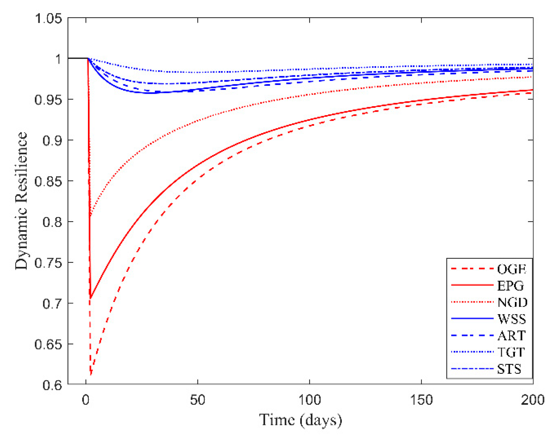
Let us suppose that the infrastructures OGE, EPG, and NGD are directly disrupted by a disaster at . The initial inoperability of the three systems is set as 0.4, 0.3, and 0.2, respectively. Other systems are not directly disrupted by the disaster. In the simulation, each time step is set as 1 day. If no restoration resources are allocated, only depending on the basic restoration capacity of the infrastructure managers, the DR of the infrastructure systems is as shown in Figure 2.
As shown in Figure 2, the DR of the directly disrupted systems (indicated by red lines) decreases sharply following the occurrence of the disaster, and the magnitude of the decrease is positively related to the initial inoperability. Owning to the basic restoration capacity of the infrastructure managers, the DR of these systems then increases with time. After approximately 100 time steps, the resilience of these systems recovers to a value greater than 0.9. Owing to interdependencies, the other infrastructure systems are indirectly disrupted. Their DR (indicated by blue lines) also first decreases and then increases. However, the resilience disturbances are relatively small as compared to those of the directly disrupted systems. The smallest DR of indirectly disrupted systems is always greater than 0.95 during the recovery process. This means that the negative impact of the events on indirectly disrupted systems is not serious. After approximately 100 time steps, the DR of the indirectly disrupted systems recovers to a value greater than 0.98. In the normal sense, only the directly disrupted infrastructure systems require extra restoration resources for system restoration, as the indirectly disrupted infrastructure systems are only functionally disrupted owing to the service dependencies on the directly disrupted systems. Therefore, in the following studies, the restoration resources are only allocated to directly disrupted systems.
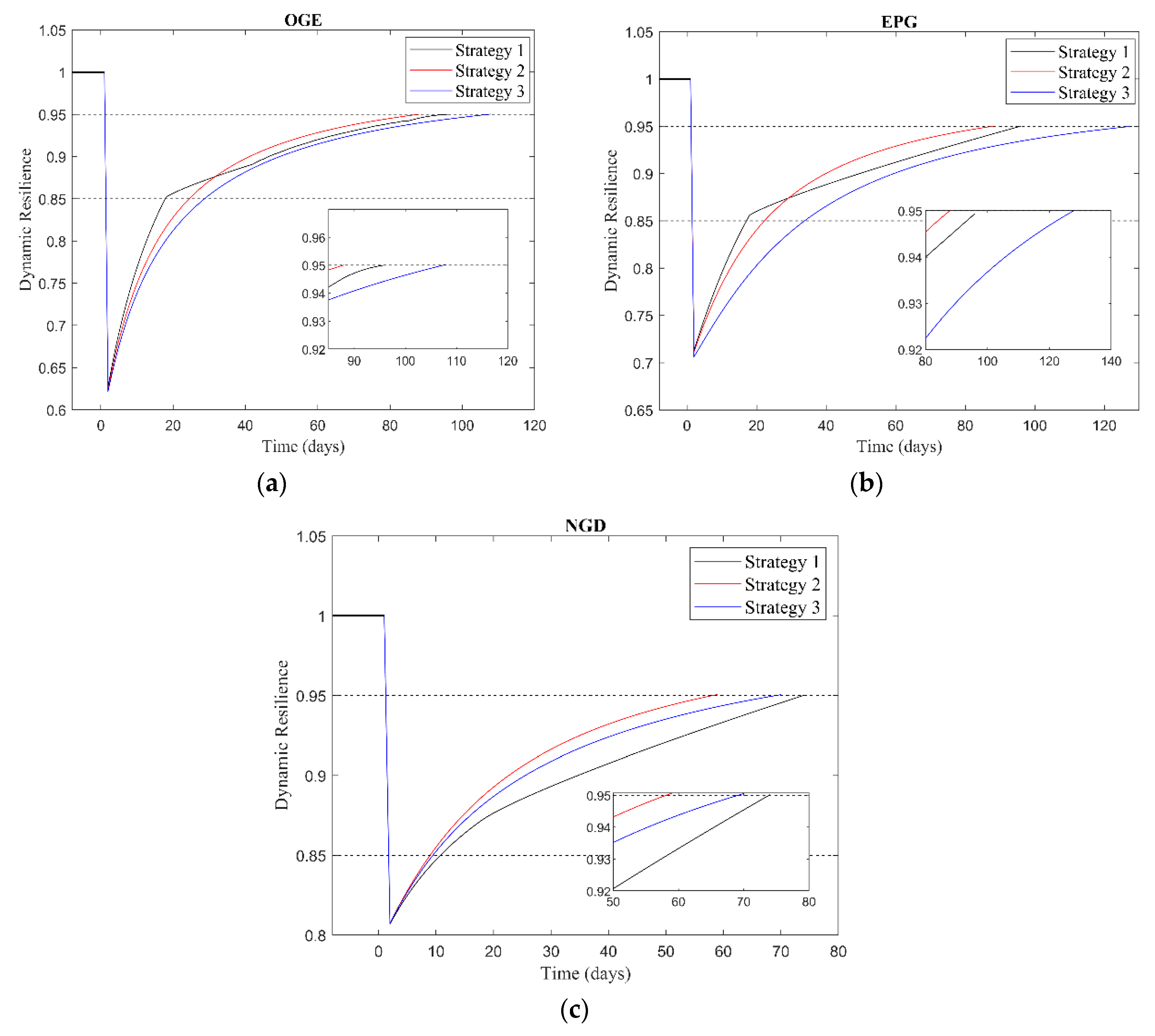
For the purpose of comparison, the DR of the infrastructure systems during the recovery process under different restoration resource allocation strategies is examined. Simulations were performed using three strategies: (1) derived from the two-stage model proposed in this study; (2) with the objective of minimizing the recovery time of infrastructure systems, to help the DR of the infrastructure systems to recover to the expected level as soon as possible; (3) with the objective of minimizing the overall loss during the recovery process of the infrastructure systems. The overall losses are the sum of the economic losses of the infrastructure systems and the usage costs of the restoration resources. Let us suppose that the restoration resource budget is 100 million dollars, the DR of the infrastructure systems during the recovery process under different strategies is as shown in Figure 3. The allocation and overall losses under different strategies are presented in Table 4.
In Figure 3, under different strategies, the time for the DR of each infrastructure system to recover to the basic level or the expected level is different. For OGE infrastructure, the time for the DR to recover to the basic level is 18, 25, and 29 time steps under different strategies. The recovery time under strategy 1 is the shortest during this recovery process. However, after 18 time steps, the slope of the DR curve of strategy 1 decreases, which means that the recovery speed of the DR under this strategy decreases. In comparison, the slopes of the DR curves of strategies 2 and 3 do not change much. The time for the DR of OGE infrastructure to recover to the expected level is 96, 88, and 108 time steps under the three strategies. The recovery time under strategy 2 is the shortest. This phenomenon can be explained by the data given in Table 4. The first objective of strategy 1 is to aid infrastructure systems’ DR to quickly recover to the basic level; when this objective is achieved, the restoration resources are reallocated to minimize the total losses in the following recovery process. In Table 4, under strategy 1, the resources allocated to OGE infrastructure are 41.85 million dollars at Stage I and 15.46 million dollars at Stage II. However, under strategy 2, the resources allocated to OGE infrastructure are always 23.32 million dollars, which is much more than that at Stage II of strategy 1. Therefore, the total recovery time under strategy 2 is the shortest. The recovery processes of EPG infrastructure are similar to those of OGE infrastructure under the three strategies.
However, the recovery processes of NGD infrastructure under the three strategies are obviously different from the other two infrastructure systems. Under strategy 2, the recovery times for the DR of NGD infrastructure to recover to the basic and expected levels are both the shortest. Moreover, the recovery time under strategy 1 is always the longest. From Table 4, it can be observed that, as the initial inoperability of NGD infrastructure is the smallest, to meet the first objective of strategy 1, all the restoration resources are allocated to OGE and EPG infrastructures at Stage I of strategy 1, and there are no resources allocated to NGD infrastructure. Thus, the time for the DR of the NGD infrastructure to recover to the basic level is the longest. Some resources are allocated to NGD infrastructure at Stage II of strategy 1. However, it is still less than that under strategy 2 and not much more than that under strategy 3; the time for the DR to recover to the expected level is still the longest under strategy 1.
In Table 4, under the three strategies, the total recovery time of the infrastructure systems is 96, 88, and 128 time steps, while the overall losses are 246.22 (128.18 + 118.04), 266.65, and 228.36 million dollars, respectively. In comparison with strategy 2, the recovery time under strategy 1 is not much longer (8 time steps), while the overall losses are much lower (28.43 million dollars). Moreover, a previous analysis showed that the times for the DR of infrastructures OGE and EPG to recover to the basic level are both shorter under strategy 1 than that under strategy 2. This means that the basic needs of users in the two infrastructure systems can be met more quickly under strategy 1. Compared with strategy 3, the recovery time under strategy 1 is much shorter (32 time steps), while the overall losses of the two strategies are close—the difference is only 9.84 million dollars. Overall, from the perspectives of meeting the needs of users and minimizing the overall losses, strategy 1 derived from the proposed model in this study is a better choice for the decision makers.
The initial inoperability of OGE infrastructure is 0.4, which is the largest among the three infrastructure systems. However, under different strategies, the resources allocated to EPG infrastructure are all higher than that allocated to OGE infrastructure. This is probably determined by the value of the cost-effectiveness parameter, which for the EPG infrastructure is 0.015; this is greater than that for the OGE infrastructure. The resources can be more effective in DR recovery if they are allocated to EPG infrastructure. However, though the cost-effectiveness parameter for NGD infrastructure is the highest, the resources allocated to this system are always the lowest. This is owing to the initial inoperability of this infrastructure being relatively small as compared to those of the other two systems.
4.3. Sensitive Analysis
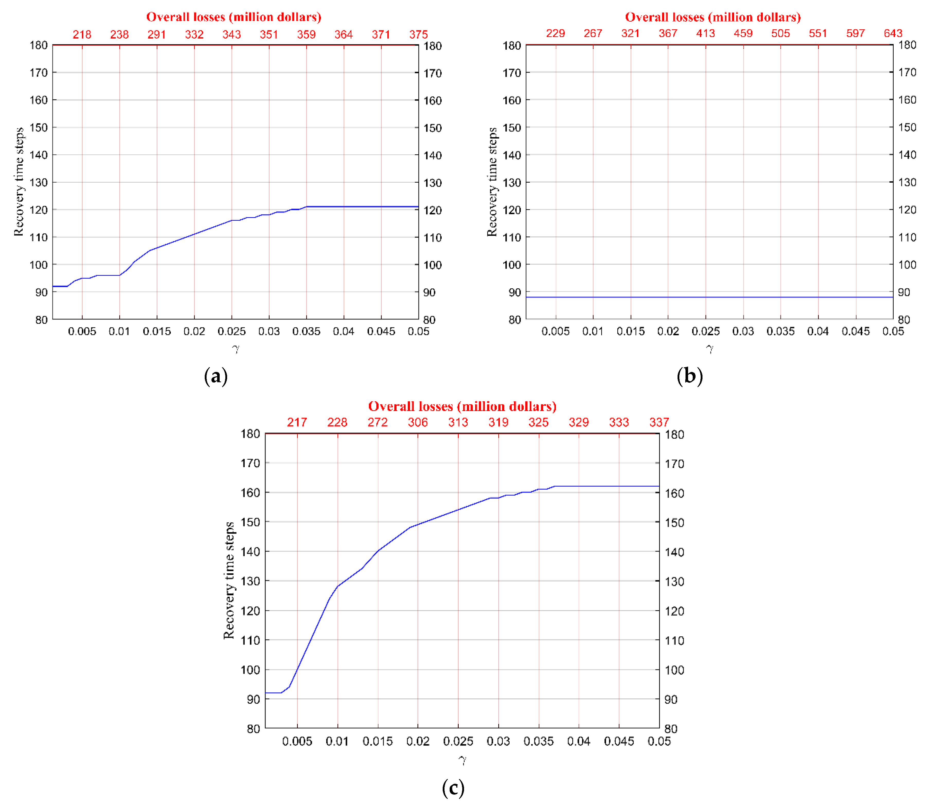
The numerical results acquired are dependent on the assumption that the value of the parameter (the usage cost of unit restoration resource in one time step) is 0.01 million dollars (per 1 million dollars in one time step). In reality, the value of the parameter is dependent on the disaster scenarios. In the following study, we explore how this parameter affects the results through a sensitivity analysis. The value of the parameter , the usage cost of unit restoration resource in one time step is set from 0.001 to 0.05 million dollars (per 1 million dollars in one time step). For different values, the recovery time of the infrastructure systems and the overall losses under the three resource allocation strategies are shown in Figure 4.
In Figure 4a, under strategy 1, the shortest recovery time of the infrastructure systems is 92 time steps, which is obtained when is 0.001. With the increase in , the recovery time increases. When is greater than 0.035, the recovery time stops increasing and remains constant at 121 time steps. This reveals that, when , with the increase in the usage cost of the restoration resources, fewer resources are allocated to the infrastructure systems. This result is consistent with the second objective of strategy 1, which is to minimize the overall losses during Stage II. When , to balance the losses of the infrastructure systems and the usage cost of the restoration resource, the resource allocation does not change with . The recovery time remains constant (121 time steps). Further, it can be observed that the overall losses keep increasing with , from 192 million dollars to 375 million dollars. When , although the recovery time of the infrastructure systems remains constant, the losses still increase with owing to the increase in the usage cost of the restoration resources.
In Figure 4b, under strategy 2, as the objective is to minimize the recovery time, the overall losses are not considered while developing the strategy, and the recovery time of the infrastructure systems remains constant for different at 88 time steps. However, the overall losses increase rapidly with , from 192 million dollars () to 643 million dollars (). For the same value, the overall losses under strategy 2 are much greater than those under strategy 1. When , the difference between the two strategies is 268 million dollars.
In Figure 4c, under strategy 3, the change in the recovery time with is similar to that under strategy 1. However, with the same , the recovery time under strategy 3 is much longer than that under strategy 1; the difference between the two is usually more than 30 time steps when . Meanwhile, the overall losses under strategy 3 are smaller than those under strategy 1. The difference between the two is usually less than 40 million dollars.
On comparing Figure 4a–c, when , the recovery time and overall losses under the three strategies are close to each other. The majority of the resources are allocated to infrastructure systems for restoration. When , the differences in the recovery time and overall losses under the three strategies become more significant with the increase in . The recovery time under strategy 2 is always the shortest, and the overall losses under strategy 3 are always the lowest. However, strategy 1 balances the satisfaction of the basic needs of the users and the reduction of overall losses. In the majority of the cases, with the same , the recovery time under strategy 1 is close to that under strategy 2, and the overall losses are close to that under strategy 3.
5. Discussion
With a limited resource budget, an optimized restoration resource allocation strategy can increase the efficiency of the recovery process of infrastructure systems and reduce the losses resulting from a disaster. Taking into consideration the government decision makers’ point of view, a two-stage restoration resource allocation model is proposed in this study. The objective of the first stage is to quickly recover the infrastructure systems’ DR to meet the basic needs of the users. The objective of the second stage is to minimize the overall losses during the recovery process following the first stage. The problem under study has several unique features over previous research: (i) the DR is applied to evaluate the effect of restoration resource efforts at each time step during the recovery process. Consequently, based on the evaluation, the stage division of resource allocation during the recovery process can be determined. (ii) The objectives of the two-stage resource allocation model are not unique during the recovery process of the infrastructure systems, which balances the recovery time and overall losses. A case study shows that the proposed model can assist decision makers in better understanding the resource allocation effects and making informed decisions following a disaster.
There are some limitations of the presented study. First, the results acquired are dependent on parameter assumptions in the proposed model, including the value of the basic and expected levels of DR. In reality, they are dependent on the characteristics of a specific infrastructure system and the needs of the users of an infrastructure service. For example, the basic level of DR for an electric power system is different from that of the water supply system; the basic level of DR for an infrastructure system serving large cities is probably higher than that serving small towns and villages. In this study, although we believe the parameter assumptions represent reality to some extent, their validity still needs to be explored using detailed data. Second, infrastructure systems are subjected to different types of disasters that could affect system performance differently. For example, earthquakes always disrupt all the infrastructure components located in the area simultaneously. Floods usually shock above-ground infrastructure components over the duration of disaster gradually. This study investigates the restoration resource allocation problem after the disaster. The type, duration and magnitude of disasters are not considered. Third, this manuscript proposes a method for resource allocation among interdependent infrastructure systems from the government’s perspective. This is very common in the case of large-scale disasters. However, in some disasters, especially small-scale disruptive events, restoration efforts of each infrastructure may be performed separately by infrastructure management organizations. Their objectives may differ from event to event. Future research will investigate how different objectives of all players in the recovery process can be considered in optimal allocation resources.
Author Contributions
Conceptualization, J.K. and C.Z.; methodology, C.Z.; software, C.Z.; validation, J.K. and C.Z.; formal analysis, J.K.; investigation, S.P.S.; resources, J.K.; data curation, C.Z.; writing—original draft preparation, C.Z.; writing—review and editing, S.P.S.; visualization, C.Z.; supervision, S.P.S.; project administration, J.K.; funding acquisition, C.Z. and S.P.S.
Funding
This research was funded by the Natural Science Foundation of China under Grant No. 71704111, Shanghai Science and Technology Development Funds under Grant No. 19692107300 and 19ZR1417300, Institute of Free Trade Zone of SUFE and Shanghai Education Committee under Grant No. 2019110183, and the Natural Sciences and Engineering Research Council (NSERC) of Canada.
Conflicts of Interest
The authors declare no conflict of interest
Notations
| Number of infrastructure systems | |
| Expected system performance level of infrastructure in monetary units | |
| Basic level of infrastructure ’s DR that meets the basic needs of the users | |
| Expected level of infrastructure ’s DR | |
| matrix, in which every entry denotes the amount of inoperability contributed by the column system to the corresponding row system owing to the interdependencies between systems | |
| Restoration resource budget | |
| Cost-effectiveness parameter denoting the effectiveness of allocating resources to infrastructure ’s recovery rate | |
| Basic restoration capacity of infrastructure ’s managers | |
| Usage cost of unit restoration resource in one time step | |
| inoperability of infrastructure systems at time t | |
| DR of infrastructure at time t | |
| Restoration resources allocated to infrastructure at Stage I | |
| Restoration resources allocated to infrastructure at Stage II | |
| Adjustment of the restoration resources allocated to infrastructure at Stage II | |
| Time at which infrastructure ’s DR recovers to its basic level | |
| Maximum value of elements in set , | |
| Time at which infrastructure ’s DR recovers to its expected level | |
| Diagonal matrix, denotes the recovery rate of infrastructure |
References
- Ouyang, M.; Dueñas-Osorio, L.; Min, X. A three-stage resilience analysis framework for urban infrastructure systems. Struct. Saf. 2012, 36, 23–31. [Google Scholar] [CrossRef]
- Murdock, H.; de Bruijn, K.; Gersonius, B. Assessment of critical infrastructure resilience to flooding using a response curve approach. Sustainability 2018, 10, 3470. [Google Scholar] [CrossRef]
- Kong, J.; Simonovic, S.P.; Zhang, C. Sequential hazards resilience of interdependent infrastructure system: A case study of Greater Toronto Area energy infrastructure system. Risk Anal. 2019, 39, 1141–1168. [Google Scholar] [CrossRef] [PubMed]
- Mao, Q.; Li, N. Assessment of the impact of interdependencies on the resilience of networked critical infrastructure systems. Nat. Hazards 2018, 4, 1–23. [Google Scholar] [CrossRef]
- Chun, H.; Chi, S.; Hwang, B. A spatial disaster assessment model of social resilience based on geographically weighted regression. Sustainability 2017, 9, 2222. [Google Scholar] [CrossRef]
- Bruneau, M.; Chang, S.E.; Eguchi, R.T.; Lee, G.C.; Rourke, T.D.; Reinhorn, A.M.; Shinozuka, M.; Tierney, K.; Wallace, W.A.; Winterfeldt, D. A framework to quantitatively assess and enhance the seismic resilience of communities. Earthq. Spectra 2003, 19, 733–752. [Google Scholar] [CrossRef]
- Bruneau, M.; Reinhorn, A.M. Exploring the concept of seismic resilience for acute care facilities. Earthq. Spectra 2007, 23, 41–62. [Google Scholar] [CrossRef]
- Chang, S.; Shinozuka, M. Measuring improvements in the disaster resilience of communities. Earthq. Spectra 2004, 20, 739–755. [Google Scholar] [CrossRef]
- Cimellaro, G.P.; Reinhorn, A.M.; Bruneau, M. Framework for analytical quantification of disaster resilience. Eng. Struct. 2010, 32, 3639–3649. [Google Scholar] [CrossRef]
- Zobel, C.W. Representing perceived tradeoffs in defining disaster resilience. Decis. Support Syst. 2011, 50, 394–403. [Google Scholar] [CrossRef]
- Henry, D.; Emmanuel, R.J. Generic metrics and quantitative approaches for system resilience as a function of time. Reliab. Eng. Syst. Saf. 2012, 99, 114–122. [Google Scholar] [CrossRef]
- Simonovic, S.P.; Peck, A. Dynamic resilience to climate change caused natural disasters in coastal megacities quantification framework. Int. J. Environ. Clim. Chang. 2013, 3, 378–401. [Google Scholar] [CrossRef] [PubMed]
- Zhang, C.; Kong, J.J.; Simonovic, S.P. Modeling joint restoration strategies for interdependent infrastructure systems. PLoS ONE 2018, 13, e0195727. [Google Scholar] [CrossRef] [PubMed]
- Sharkey, T.C.; Nurre, S.G.; Nguyen, H.; Chow, J.H.; Mitchell, J.E.; Wallace, W.A. Identification and classification of restoration interdependencies in the wake of Hurricane Sandy. J. Infrastruct. Syst. 2015, 22, 04015007. [Google Scholar] [CrossRef]
- Mackenzie, C.A.; Baroud, H.; Barker, K. Optimal resource allocation for recovery of interdependent systems: Case study of the Deepwater Horizon oil spill. In Proceedings of the 2012 Industrial and Systems Engineering Research Conference, Orlando, FL, USA, 19–23 May 2012. [Google Scholar]
- Mackenzie, C.A.; Baroud, H.; Barker, K. Static and dynamic resource allocation models for recovery of interdependent systems: Application to the Deepwater Horizon oil spill. Ann. Oper. Res. 2016, 236, 103–129. [Google Scholar] [CrossRef]
- Zhang, C.; Liu, X.; Jiang, Y.P. A two-stage resource allocation model for lifeline systems quick response with vulnerability analysis. Eur. J. Oper. Res. 2016, 250, 855–864. [Google Scholar] [CrossRef]
- Zhang, C.; Kong, J.J.; Simonovic, S.P. Restoration resource allocation model for enhancing resilience of interdependent infrastructure systems. Saf. Sci. 2018, 108, 169–177. [Google Scholar] [CrossRef]
- Baroud, H.; Barker, K.; Ramirez-Marquez, J.E. Inherent costs and interdependent impacts of infrastructure network resilience. Risk Anal. 2015, 35, 642–662. [Google Scholar] [CrossRef]
- Johansson, J.; Hassel, H. An approach for modelling interdependent infrastructures in the context of vulnerability analysis. Reliab. Eng. Syst. Saf. 2010, 95, 1335–1344. [Google Scholar] [CrossRef]
- Ouyang, M. Review on modeling and simulation of interdependent critical infrastructure systems. Reliab. Eng. Syst. Saf. 2014, 121, 43–60. [Google Scholar] [CrossRef]
- Rosato, V.; Issacharoff, L.; Tiriticco, F.; Meloni, S. Modelling interdependent infrastructures using interacting dynamical models. J. Infrastruct. Syst. 2008, 4, 63–79. [Google Scholar] [CrossRef]
- González, A.D.; Leonardo, D.; Sánchez-Silva, M. The Interdependent Network Design Problem for Optimal Infrastructure System Restoration. Comput. Civ. Infrastruct. Eng. 2016, 31, 334–350. [Google Scholar] [CrossRef]
- Duchin, F. Resources for sustainable economic development: A framework for evaluating infrastructure system alternatives. Sustainability 2017, 9, 2105. [Google Scholar] [CrossRef]
- Haimes, Y.Y.; Horowitz, B.M.; Lambert, J.H. Inoperability input-output model for interdependent infrastructure sectors. I: Theory and methodology. J. Infrastruct. Syst. 2005, 11, 67–79. [Google Scholar] [CrossRef]
- Rinaldi, S.M.; Peerenboom, J.P.; Kelly, T.K. Identifying, understanding, and analyzing critical infrastructure interdependencies. IEEE Control Syst. Mag. 2001, 21, 11–25. [Google Scholar]
- Bialas, A. Risk management in critical infrastructure—Foundation for its sustainable work. Sustainability 2016, 8, 240. [Google Scholar] [CrossRef]
- Leonardo, D.; Kwasinski, A. Quantification of lifeline system interdependencies after the 27 February 2010 M w 8.8 offshore Maule, Chile, earthquake. Earthq. Spectra 2012, 28, S581–S603. [Google Scholar]
- Lin, Y.K.; Pfund, M.E.; Fowler, J.W. Heuristics for minimizing regular performance measures in unrelated parallel machine scheduling problems. Comput. Oper. Res. 2011, 38, 901–916. [Google Scholar] [CrossRef]
- Lian, C.; Haimes, Y.Y. Managing the risk of terrorism to interdependent infrastructure systems through the dynamic inoperability input–output model. Syst. Eng. 2006, 9, 241–258. [Google Scholar] [CrossRef]
- Li, Y.F.; Tang, C.C.; Peeta, S.; Wang, Y.B. Nonlinear consensus based connected vehicle platoon control incorporating car-following interactions and heterogeneous time delays. IEEE Trans. Intell. Transp. 2019, 20, 2209–2219. [Google Scholar] [CrossRef]
Figure 1.
Typical performance of an infrastructure system after a disaster.

Figure 2.
The dynamic resilience (DR) of infrastructure systems without restoration resources.

Figure 3.
The DR of infrastructure systems during the recovery process under different strategies: (a) OGE; (b) EPG; (c) NGD.
Figure 3.
The DR of infrastructure systems during the recovery process under different strategies: (a) OGE; (b) EPG; (c) NGD.

Figure 4.
Recovery time and the overall losses under the three strategies with different values (a) under strategy 1; (b) under strategy 2; (c) under strategy 3.
Figure 4.
Recovery time and the overall losses under the three strategies with different values (a) under strategy 1; (b) under strategy 2; (c) under strategy 3.


Table 1.
Infrastructure systems selected for the case study.
| Symbol | Name |
|---|---|
| OGE | Oil and gas extraction |
| EPG | Electric power generation, transmission, and distribution |
| NGD | Natural gas distribution |
| WSS | Water, sewage, and other systems |
| ART | Air, rail, water, and truck transportation |
| TGT | Transit and ground passenger transportation |
| STS | Scenic transportation and support activities for transportation |
Table 2.
Average daily performance of infrastructure systems (in millions of dollars).
| OGE | EPG | NGD | WSS | ART | TGT | STS | Exogenous Demand | Performance Output | |
|---|---|---|---|---|---|---|---|---|---|
| OGE | 1.285 | 2.489 | 3.237 | 0 | 0 | 0.16 | 0 | 2.957 | 10.13 |
| EPG | 0.759 | 1.725 | 3.200 | 0.156 | 0.798 | 0.264 | 0.287 | 4.115 | 11.30 |
| NGD | 2.078 | 1.790 | 0.380 | 2.266 | 0.784 | 0.138 | 0.914 | 5.110 | 13.46 |
| WSS | 0.444 | 1.079 | 0.801 | 0.182 | 0.330 | 0.295 | 0.101 | 3.791 | 7.02 |
| ART | 0.502 | 0.807 | 0.407 | 0.261 | 2.501 | 0.44 | 1.492 | 1.639 | 8.05 |
| TGT | 0 | 0.145 | 0.067 | 0.128 | 0.192 | 0 | 2.224 | 2.277 | 5.03 |
| STS | 0.481 | 2.203 | 0.478 | 0.06 | 2.260 | 0.146 | 2.025 | 6.557 | 14.21 |
| Value Added | 4.579 | 1.066 | 4.890 | 3.970 | 1.184 | 3.590 | 7.167 | ||
| Performance Input | 10.13 | 11.30 | 13.46 | 7.02 | 8.05 | 5.03 | 14.21 |
Table 3.
Parameters in the two-stage resource allocation model.
| Infrastructure | OGE | EPG | NGD | WSS | ART | TGT | STS |
|---|---|---|---|---|---|---|---|
| Expected performance (in million dollars) | 10.13 | 11.3 | 13.46 | 7.02 | 8.05 | 5.03 | 14.21 |
| Basic restoration capacity | 0.1 | 0.2 | 0.15 | 0.1 | 0.1 | 0.1 | 0.1 |
| Cost-effectiveness parameter (per $1 million) | 0.01 | 0.015 | 0.02 | 0.01 | 0.01 | 0.01 | 0.01 |
Table 4.
Resource allocation and overall losses under different strategies.
| Strategy 1 (Stage I) | Strategy 1 (Stage II) | Strategy 2 | Strategy 3 | |
|---|---|---|---|---|
| Resources allocated to OGE (million dollars) | 41.85 | 15.46 | 23.32 | 13.27 |
| Resources allocated to EPG (million dollars) | 58.15 | 18.35 | 70.29 | 20.11 |
| Resources allocated to NGD (million dollars) | 0 | 5.33 | 6.39 | 4.3 |
| Total resources allocated (million dollars) | 100 | 39.14 | 100 | 37.68 |
| Overall losses (million dollars) | 128.18 | 118.04 | 266.65 | 228.36 |
| Recovery time (time steps) | 18 | 78 | 88 | 128 |
© 2019 by the authors. Licensee MDPI, Basel, Switzerland. This article is an open access article distributed under the terms and conditions of the Creative Commons Attribution (CC BY) license (http://creativecommons.org/licenses/by/4.0/).
Share and Cite
MDPI and ACS Style
Kong, J.; Zhang, C.; Simonovic, S.P. A Two-Stage Restoration Resource Allocation Model for Enhancing the Resilience of Interdependent Infrastructure Systems. Sustainability 2019, 11, 5143. https://doi.org/10.3390/su11195143
AMA Style
Kong J, Zhang C, Simonovic SP. A Two-Stage Restoration Resource Allocation Model for Enhancing the Resilience of Interdependent Infrastructure Systems. Sustainability. 2019; 11(19):5143. https://doi.org/10.3390/su11195143
Chicago/Turabian StyleKong, Jingjing, Chao Zhang, and Slobodan P. Simonovic. 2019. "A Two-Stage Restoration Resource Allocation Model for Enhancing the Resilience of Interdependent Infrastructure Systems" Sustainability 11, no. 19: 5143. https://doi.org/10.3390/su11195143
Note that from the first issue of 2016, this journal uses article numbers instead of page numbers. See further details here.