Multi-Scale Assessment of Relationships between Fragmentation of Riparian Forests and Biological Conditions in Streams

Abstract

Due to anthropogenic activities within watersheds and riparian areas, stream water quality and ecological communities have been significantly affected by degradation of watershed and stream environments. One critical indicator of anthropogenic activities within watersheds and riparian areas is forest fragmentation, which has been directly linked to poor water quality and ecosystem health in streams. However, the true nature of the relationship between forest fragmentation and stream ecosystem health has not been fully elucidated due to its complex underlying mechanism. The purpose of this study was to examine the relationships of riparian fragmented forest with biological indicators including diatoms, macroinvertebrates, and fish. In addition, we investigated variations in these relationships over multiple riparian scales. Fragmentation metrics, including the number of forest patches (NP), proportion of riparian forest (PLAND), largest riparian forest patch ratio (LPI), and spatial proximity of riparian forest patches (DIVISION), were used to quantify the degree of fragmentation of riparian forests, and the trophic diatom index (TDI), benthic macroinvertebrates index (BMI), and fish assessment index (FAI) were used to represent the biological condition of diatoms, macroinvertebrates, and fish in streams. PLAND and LPI showed positive relationships with TDI, BMI, and FAI, whereas NP and DIVISION were negatively associated with biological indicators at multiple scales. Biological conditions in streams were clearly better when riparian forests were less fragmented. The relationships of NP and PLAND with biological indicators were stronger at a larger riparian scale, whereas relationships of LPI and DIVISION with biological indicators were weaker at a large scale. These results suggest that a much larger spatial range of riparian forests should be considered in forest management and restoration to enhance the biological condition of streams.

1. Introduction

Land use patterns with strongly fragmented forests or no forests located in stream riparian areas have significant negative impacts on water quality and aquatic ecological communities [1,2,3,4] due to alteration of stream environments and sediment run-off mechanisms, pollution, and nutrient loading [5,6,7,8,9]. Thus, land use within riparian areas has become a key concern for stream management and restoration [10]. Previous research has shown that streamside forests affect aquatic ecosystems by providing substantial amounts of energy and woody debris [11,12,13,14,15]. Some previous studies have demonstrated that land use within riparian areas threatens ecosystems through fragmentation of forests and degradation of soil and water properties [16,17,18,19]. Therefore, it is evident that riparian forests play an important role as corridors connecting fragmented forests and stream habitats. Furthermore, forest fragmentation within riparian areas has been directly linked with degraded water quality and stream ecosystem health [8,11,20,21,22], and spatiotemporal changes in land use, logging, intensive forest management, and rapid economic development have played significant roles in accelerating forest fragmentation [23,24,25,26,27]. Human activities in forested areas affect various stream characteristics, such as the microclimate, local air temperature, stream water temperature, humidity, wind speed [28,29], and concentrations of nutrients, sediments, and pollutants in streams, as well as ecological conditions [8,11,30,31,32,33,34,35,36]. However, the main characteristics of the relationship between forest fragmentation and stream ecosystems remain poorly understood, because they are associated through complex mechanisms involving numerous other factors (e.g., climate, geology, topography, and hydrological processes) [37,38,39,40].

Many previous studies have focused on a particular aspect of watershed forests (i.e., proportion of forested area), and have fallen short of identifying which aspects of fragmentation have the strongest impacts on stream biota. For example, Allan (2004) [41] showed that a greater proportion of forest cover within a watershed was positively linked with various stream conditions. Roy et al. (2003) [42] reported that decreased forest cover was related to degradation of biotic integrity in streams. Furthermore, Kim et al. (2014) [43] reported that the effects of forests at large spatial scales (i.e., forest width) are more important to fish than at small scales. Fragmentation can be characterized as a function of the patch number within a given area, patch size, patch shape, and the spatial distribution of patches [44,45,46]. Specifically, forest fragmentation can be characterized as forest loss, increased edge areas, decreased size and core area, non-contiguous splitting of large forest areas into smaller fragmented forest patches, and increased distance between patches [47,48].

When investigating the relationships of various land uses and their spatial patterns in riparian areas with stream organisms, identifying the optimal spatial scale is one of the most critical and fundamental issues. In landscape ecology, scale can be defined by two factors, extent and grain size, which vary in time and space. In cross-sectional studies, extent defines the spatial range of the investigation, whereas grain size refers to the unit of analysis. Scale has been a central concept in landscape ecology, as landscape structure and function are scale dependent [49,50]. Often, scientists have preferred to use multiple spatial scales (i.e., extents) to examine relationships between land use types and stream health, as there is no known scale of the relationship [51,52,53]. Allan et al. (1997) [54] discussed how human activities at various spatial scales impact the stream environment and organisms in streams. The extent of fragmentation is critical to understanding the relationship between forest fragmentation and local ecological processes in streams and surrounding areas [55]. In part, this importance is due to the extent of fragmentation negatively affecting biological integrity by increasing the exposure of streams to light and wind and increasing stresses on aquatic ecosystems caused by temperature fluctuations. Therefore, this work is essential to clarify the extent to which forest fragmentation affects stream environments and organisms in streams. For example, forests hundreds of meters away from streams are associated with the supply of coarse sediments and organic matter, whereas shade from riparian forests can lower water temperatures [56]. Arguably, forest fragmentation in riparian areas may have more significant impacts on stream ecosystems than in other forest types throughout the watershed simply due to stream proximity [2,57,58]. Rich evidence indicates that riparian forests have positive effects, including stream bank stabilization [59], decreasing nutrient and sediment loads from riparian areas [60,61], lowering stream water temperature [62], providing habitat [63], and enhancing biodiversity in streams [64]. Recently, Yirigui et al. (2019) [8] reported that forest fragmentation within a 500-m buffer zone has significant negative effects on biological indicators in streams. According to their study, fragmentation of riparian forests may lower their efficiency for filtering and absorbing nutrients, sediments, and pollutants, resulting in poor stream water quality and biological condition. However, the extent to which riparian fragmented forest affects the biological condition of streams remained unclear. Answering this question is essential for planners and managers to make critical decisions regarding effective stream management and restoration strategies.

In this study, we investigated the relationships of forest fragmentation with biological indicators including diatoms, macroinvertebrates, and fish over multiple riparian scales. In addition, we examined the variation in relationships between riparian forest fragmentation and biological indicators for streams over different spatial scales (i.e., extents). The degree of forest fragmentation in riparian areas was assumed to impact the effectiveness of various mechanisms (e.g., filtering, absorbing, and up-taking) of riparian forests, as well as hydrological and biochemical runoff processes [8,65,66,67,68], resulting in degraded stream environments (e.g., high levels of pollutants, nutrients, and sediments) and poor biological indicators [37,69,70,71,72,73,74,75]. Additionally, we hypothesized that the negative influence of forest fragmentation on biological conditions in streams may vary with riparian buffer size due to the proximity of streams.

2. Materials and Methods

2.1. Study Areas

The Korean peninsula is located between 33°7′ and 43°1′ N latitude, and 124°11′ and 131°53′ E longitude. The area of the Korean Peninsula is 221,000 km², and approximately 45% is within South Korea. The Nakdong River Basin is located between 35°03′and 37°13′ north latitudes and between 127°29′ and 129°18′ east longitudes, accounting for about 25% of South Korea’s total geographical area. The Nakdong River system, one of the major river systems in South Korea, occupies the southeastern region and its basin area is 23,702 km²; the Nakdong is also the longest river in Korea, with a length of 511 km [76]. The study area is composed of four major land cover types: commercial (0.2%), agricultural (23.5%), industrial (0.5%), and forest (70.3%). Korean forests were badly degraded during the first half of the 20th century due to watershed urbanization processes, the transition from forest to farmland, dam building, and other processes. These land uses gradually led to increasingly serious degradation of aquatic ecosystems. Total annual precipitation in the basin is 1200 mm, and about 60% of the annual precipitation falls in summer (June to September). The mean depth and flow velocity of the Nakdong River are 47.41 cm and 39.19 cm/s, respectively [43]. The Nakdong river basin has been the focal area of investigation for relevant study areas because the river has been experiencing serious changes in biochemical and physical conditions, such as degraded water quality, increasing algal blooming frequency, decreased flow speed, increased water temperature, increased residence time, and changes in species composition of diatom, macroinvertebrate, and fish in the river since Korean government placed 8 large weirs in 2012 (https://en.wikipedia.org/wiki/FourMajor_Rivers_Project, accessed on 13 August 2019).

2.2. Sampling Sites

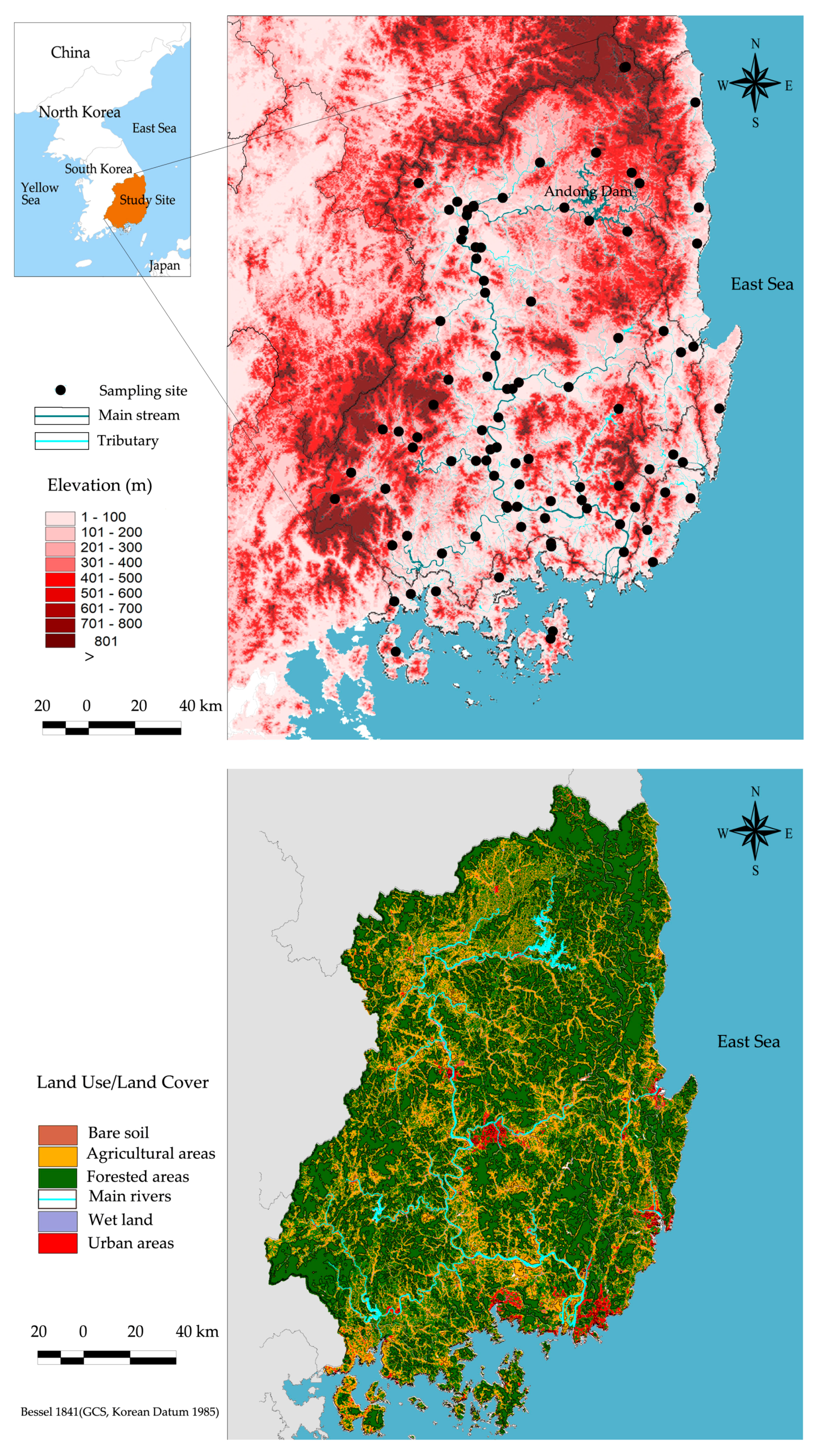
In this study, biological indicators were extracted from MOE (Ministry of Environment) datasets maintained under the National Aquatic Ecological Monitoring Program (NAEMP). NAEMP has been used to monitor biological conditions of streams in Korea since 2007 [77]. Three assemblages (diatoms, macroinvertebrates, and fish) were extensively surveyed in the Nakdong River system and sampled twice annually [78,79]. We used biological indicator datasets collected in 2014 that aligned with land use data released by MOE for this study. To compute fragmentation metrics, we selected sampling sites with at least two riparian forest patches, resulting in 79 monitoring sites (Figure 1).

2.3. Biological Indicators and Fragmentation Metrics

In this study, we used diatoms (trophic diatom index, TDI), macroinvertebrates (benthic macroinvertebrates index, BMI), and fish (fish assessment index, FAI) as indicators of the biological condition of streams in the study area. TDI is an index used for monitoring trophic condition in freshwater ecosystems based on the percentages of benthic diatom taxa, estimating periphyton condition in streams based on species abundance and sensitivity [53,74,80,81]. BMI describes the condition of benthic macroinvertebrate assemblages based on changes in habitat and environmental condition [82,83,84]. BMI uses a number assigned to each species, the unit saprobic value, and the frequency as weighting indicators for the species. As part of their long-term monitoring program, MOE developed BMI and then applied weighting factors and saprobic values to the macroinvertebrate index [79]. Fish are especially good indicators of environmental quality [85]. The NAEMP analyzed properties related to the ecological characteristics of Korean fish assemblages and adopted eight metrics into the Fish Assessment Index (FAI) [86]. TDI, BMI, and FAI scores (see

Table 1. Equations for computing biological indicators, from National Aquatic Ecological Monitoring Program (NAEMP) [87].

Biological Indicators	Equations
Trophic diatom index (TDI)	TDI = 100 − {(WMS × 25) − 25} WMS: weighted mean sensitivity $\mathrm{WMS}={\displaystyle \sum }{\mathrm{A}}_{\mathrm{j}}·{\mathrm{S}}_{\mathrm{j}}·\frac{{\mathrm{V}}_{\mathrm{j}}}{{\displaystyle \sum }{\mathrm{A}}_{\mathrm{j}}·{\mathrm{V}}_{\mathrm{j}}}$ where, j = species Aj = abundance (proportion) of species j in the sample (%) Sj = pollution sensitivity (1 ≤ S ≤ 5) of species j Vj = indicator value (1 ≤ V ≤ 3)
Benthic macroinvertebrates index (BMI)	$\mathrm{BMI}=\left\{4-{\displaystyle \sum _{\mathrm{j}=1}^{\mathrm{n}}}{\mathrm{S}}_{\mathrm{j}}{\mathrm{H}}_{\mathrm{j}}{\mathrm{G}}_{\mathrm{j}}/{\displaystyle \sum _{\mathrm{j}=1}^{\mathrm{n}}}{\mathrm{H}}_{\mathrm{j}}{\mathrm{G}}_{\mathrm{j}}\right\}\times 25$ where, j = number assigned to species n = number of species Sj = unit saprobic value of species j Hj = frequency of species j Gj = indicators weight value of species j
Fish assessment index (FAI)	FAI = sum of 8 metrics. Metric 1 (M1): number of Korean native species Metric 2 (M2): number of rifle benthic species Metric 3 (M3): number of sensitive species Metric 4 (M4): percentage of tolerant species Metric 5 (M5): percentage of omnivores Metric 6 (M6): percentage of insectivores Metric 7 (M7): the amount of collection native species Metric 8 (M8): percentage of fish abnormalities

for the method used to compute scores for each index) ranged from 0 to 100 and were classified into four classes: Class A (excellent), Class B (Good), Class C (Fair), and Class D (Poor) [79].

2.4. Multi-scale Measurements

Stream biota were not only affected by the amount of forested area but also the width (i.e., scale) of riparian areas adjacent to streams [88,89]. Various landscape indicators are known to have differing effects at different scales, suggesting that stream ecosystem management requires the application of multi-scale analysis [90]. Multi-scale applications are widely employed for watershed land use management, allowing different landscape perspectives to be assessed by applying landscape metrics to assess fragmentation and its effects [91,92]. We utilized the buffer width required for drinking water protection under Korean MOE regulations. Since 1999, the Korean MOE has used two buffer widths (500 m in developed areas and 1 km in rural and semi-natural areas) to preserve riparian areas and protect drinking water quality [11,43]. Because most of the sampling sites used in the study were located in rural and semi-natural areas, we used a 1-km buffer as the base riparian scale. Recently, Kim et al. (2014) [43] studied the relationship between land use and fish by analyzing land use types within a 5-km buffer around the river. Based on these factors, we selected two scales (1 and 5 km) and one intermediate scale of 2 km to investigate the relationships among biological indicators.

2.5. Measuring Forest Fragmentation

The proportions of urban, paddy field, dry field, forest, grass, wetland, and bare soil were extracted from a digital Korean land use land cover map (LULC) using ArcGIS software version 10.1. This map was generated using Landsat Thematic Mapper (TM; 30-m resolution) and Indian Remote Sensing (IRS)-1C pan-chromatic (5.8-m resolution) images [93]. The LULC map was categorized into forests and non-forests in a grid format (resolution = 50 m). Riparian forest grids for each sampling site were extracted at three riparian scales, and then the selected fragmentation metrics were computed using FRAGSTATS 4.3, a spatial pattern metrics computing program [94]. The pattern metrics selected to quantify the degree of forest fragmentation included the largest patch index (LPI), the number of patches (NP), the proportion of forest (PLAND), and the division index (DI) at the class level [95,96,97,98,99,100].

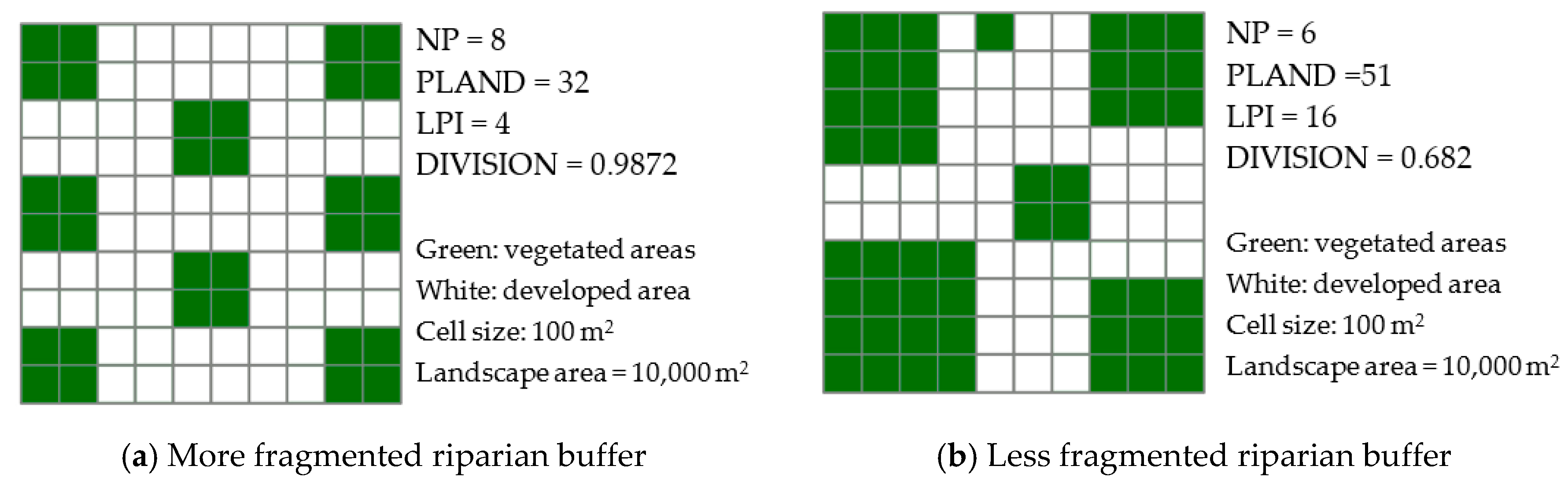
Both patch area and patch density metrics are important, as they provide essential information about fragmentation [46,96]. The simplest fragmentation metric is the number of forest patches (NP), which describes whether the forest area is currently fragmented. PLAND quantifies the percentage of the entire buffer that is composed of forest patches. PLAND is a fundamental measure of landscape composition, showing the scope of the landscape that is made up of riparian forest patches. For this study, it was important to clarify how much forest was present within the riparian areas. LPI is a measure of dominance and is computed as the percentage of the largest forest patch over the total buffer area. Large undivided forest areas must be considered when planning land use in streamside areas. DIVISION represents the proportion of the riparian area composed of forest patches, and it decreases as distance among forest patches increases. In general, the values of PLAND and LPI are negative metrics, as higher values indicate low fragmentation. Conversely, NP and DIVISION are positive metrics, with greater values indicating higher degrees of fragmentation (

Table 2. Metrics to quantify forest fragmentation [101].

Fragmentation Characteristics	Acronym	Equation	Remarks
Number of riparian patches	NP	ni	NP ≥ 1, without limit. High NP value = greater degree of fragmentation.
Proportion riparian forest	PLAND	$\left({\displaystyle \sum _{\mathrm{i}=1}^{\mathrm{n}}}{\mathrm{a}}_{\mathrm{i}}/\mathrm{A}\right)\times 100$	0 < PLAND ≤ 100 0 = no riparian forests.
Largest riparian forest patch ratio	LPI	$\underset{\mathrm{i}=1}{\max }({\mathrm{a}}_{\mathrm{i}})/\mathrm{A}\times \left(100\right)$	0 < LPI ≤ 100 0 = greater degree of fragmentation.
Spatial proximity of riparian forest patches	DIVISION	$\left\{1-{\displaystyle \sum _{\mathrm{i}=1}^{\mathrm{n}}}{\left({\mathrm{a}}_{\mathrm{i}}/\mathrm{A}\right)}^2\right\}$	0 ≤ DIVISION < 1 0 = a single forest patch.

n = number of forest patches, a_i = size of riparian forest patch i, and A = total buffer size.

). Figure 2 illustrates differences among fragmentation metrics, including NP, PLAND, LPI, and DIVISION, with conceptual diagrams of less and more fragmented riparian vegetation areas.

2.6. Data Analysis

Confirmation of the normality of the observed variables was conducted using the z-score normality test method, which resulted in Zskewness and Zkurtosis values of 3.92 for medium-sized observation datasets (50 < # of observation < 300) [101,102]. In this test, Zskewness or Zkurtosis values exceeding 3.92 indicate that the distribution of an observed variable differs significantly from the normal distribution (p < 0.05). Because preliminary analysis using the z-score normality test indicated that the distributions of some of the variables used in the study were non-normal, we adopted the non-parametric Spearman’s rho rank correlation test to account for non-normal distributions using the cor.test() function and ggpubr package in R. Then, to visualize these correlations, we applied the base R “pairs” function to create matrices of scatterplots. We utilized the bootstrapping resampling method to compute confidence intervals for the estimated correlations due to the relatively small number of observations collected over large study areas [103]. Bootstrapping was carried out using the boot package in R using 1000 resamples (for more details about the bootstrap resampling method and statistics, see [104,105]). Bootstrap techniques have been used in related fields, such as hydrologic processes (e.g., [106]), material transport (e.g., [107,108]) and water quality (e.g., [109,110,111]). The significance of bootstrap correlation coefficients between biological indicators and fragmentation metrics at various scales was tested using the Z-value method [112]. Redundancy analysis (RDA) was conducted to evaluate the relationships of TDI, BMI, and FAI with fragmentation metrics using the vegan, ggplot2, and ggrepel R packages. Redundancy analysis (RDA) is a method combining regression and principal component analysis (PCA). RDA is a direct gradient analysis method for evaluating linear relationships between multiple dependent and independent variables. RDA complements hierarchical partitioning by allowing for exploration of associations among all response and explanatory variables [113,114,115].

3. Results

3.1. Descriptive Statistics of Biological Indicators

NAEMP defines poor values as 0 ≤ TDI < 30, 0 ≤ BMI < 45, and 0 ≤ FAI < 25. The study area exhibited minimum TDI, BMI, and FAI values of 7.80, 13.70, and 12.50, respectively. This result means that some sampling sites have very poor biological conditions. Meanwhile, NAEMP defines excellent values as 60 ≤ TDI ≤ 100, 80 ≤ BMI ≤ 100, and 87.5 ≤ FAI < 100. The corresponding maximum values of the biological indicators were 76.30, 91.90, and 90.70, respectively. Descriptive statistics of the biological indicators suggest that the biological condition of Nakdong River varies among sites (

Table 3. Descriptive statistics of stream biological indicators.

Biological Indicators	Min.	Max.	Mean ± S.D.	Z-Score Normality Test 1)
				Zskewness	Zkurtosis
TDI	7.80	76.30	46.22 ± 15.95	−1.17	−0.27
BMI	13.70	91.90	68.21 ± 16.7	−3.54 *	1.23
FAI	12.50	90.70	50.52 ± 18.99	0.90	1.23

n = 79. S.D. = Standard Deviation. * p < 0.05. ¹⁾ p < 0.05, if Z_skewness or Z_kurtosis > 3.26.

). Most TDI values were distributed around the mean values. The patterns of TDI and FAI showed similar symmetric phenomena, suggesting that diatoms and fish were more frequently at the fair level than at the good level (45 ≤ TDI < 60, 25 ≤ FAI < 56.2) or poor level (0 ≤ TDI < 30, 0 ≤ FAI < 25). Poor values of TDI and FAI were observed at the majority of sampling sites. BMI showed a relatively normal distribution, and the maximum and minimum values of the biological indicators showed that biological conditions are generally not good. The z-scores of skewness and kurtosis [101,102] indicated normal distributions for the observed biological indicators, despite the asymmetric distribution of BMI (Table 3).

3.2. Descriptive Statistics of Forest Fragmentation Metrics at Multiple Scales

Table 4. Descriptive statistics of forest fragmentation metrics at three spatial scales.

Scale	Biological Indicators	Min.	Max.	Mean ± S.D.	Z-Score Normality Test 1)
					Zskewness	Zkurtosis
1 km scale	NP	2	30	7.92 ± 5.07	5.99 *	7.96 *
	PLAND	1.27	81.87	32.82 ± 20.47	2.08	−0.84
	LAI	0.58	81.75	19.08 ± 13.77	5.56 *	8.20 *
	DIVISION	0.33	1	0.93 ± 0.1	5.56 *	1.74
2 km scale	NP	2	67	21.25 ± 12.45	4.61 *	4.03 *
	PLAND	4.01	88.78	43 ± 10.92	0.73 *	−0.98
	LAI	0.65	87.49	21.04 ± 14.61	7.55 *	1.70
	DIVISION	0.23	1	0.91 ± 0.12	−12.54 *	27.88 *
5 km scale	NP	9	272	89.27 ± 62.75	1.16	4.20 *
	PLAND	9.16	89.45	53.57 ± 16.22	0.41	−0.34
	LPI	1.87	85.24	21.18 ± 14.66	3.45 *	8.97 *
	DIVISION	0.27	1	0.91 ± 0.11	−11.47 *	23.62 *

n = 79. S.D. = Standard Deviation. * p < 0.05. ¹⁾ p < 0.05, if Z_sknewness or Z_kurtosis > 3.26.

provides a descriptive statistical summary of forest landscape condition at spatial scales of 1 km, 2 km, and 5 km. Mean values of the forest metrics showed consistent increases with increasing scale. For example, NP values for spatial scales of 1 km, 2 km, and 5 km are 7.92, 21.25, and 89.27, respectively, whereas PLAND values are 32.82, 43, and 53.57, respectively. However, the mean values of DIVISION (0.93, 0.91, and 0.91, respectively) and LPI (19.08 21.04, and 21.18, respectively) showed no notable differences among these three spatial scales. Meanwhile, the maximum values of NP (30, 67, and 272, respectively), PLAND (81.87, 88.78, and 89.45, respectively), and LPI (81.75, 87.49, and 85.24, respectively) indicate the very weak relationship between the mean value and maximum value of each scale. The DIVISION index is near 1, confirming extensive forest fragmentation in the study area. Meanwhile, the correlation of larger scales with a greater number of patches confirmed that larger forests exhibit more forest fragmentation. PLAND is made up of numerous forest area characteristics for the indicated fragmentation condition. Increasing patch numbers also supported a higher degree of fragmentation in the forest pattern. The decrease of LPI revealed a similar tendency. Thus, deforestation was likely responsible for the increase in forest fragmentation. High values of LPI suggest that the region is less fragmented [12,46]. These results revealed growing forest fragmentation in the Nakdong River watershed. The z-scores of skewness and kurtosis of the observed fragmentation metrics showed that the distribution of PLAND followed a normal distribution at all scales, whereas the distributions of NP, LPI, and DIVISION were inconsistent among scales. In particular, the relatively high Z_skewness and Z_kurtosis values of DIVISION indicated high asymmetry and strongly peaked shapes at scales of 2 km and 5 km (Table 4). The non-normal distributions of some of fragmentation metrics suggested that conventional parametric statistics might not be suitable for this study.

3.3. Correlations between Biological Indicators and Fragmentation Metrics

Table 5. Correlation coefficients and confidence intervals of correlations between biological indicators and forest fragmentation metrics at multiple scales.

TDI
Fragmentation Metrics	1 km Scale		2 km Scale		5 km Scale
	Correlation	Confidence Interval 1)	Correlation	Confidence Interval 1)	Correlation	Confidence Interval 1)
NP	0.00	(−0.22, 0.18)	−0.02	(−0.24, 0.15)	−0.27 *	(−0.50, −0.08)
PLAND	0.35 **	(0.14, 0.54)	0.42 **	(0.15, 0.56)	0.40 **	(0.17, 0.56)
LPI	0.33 **	(0.13, 0.50)	0.31 **	(0.02, 0.43)	0.24 **	(0.04, 0.40)
DIVISION	−0.34 **	(−0.45, −0.13)	−0.35 **	(−0.43, −0.08,)	−0.29 **	(−0.42, −0.11,)
BMI
Fragmentation Metrics	1 km Scale		2 km Scale		5 km Scale
	Correlation	Confidence Interval 1)	Correlation	Confidence Interval 1)	Correlation	Confidence Interval 1)
NP	0.00	(−0.28, 0.19)	−0.04	(−0.14, 0.23)	−0.23 *.	(−0.36, 0.12)
PLAND	0.40 **	(0.13, 0.51)	0.42 **	(0.17, 0.53)	0.46 **	(0.21, 0.56)
LPI	0.38 **	(0.09, 0.47)	0.38 **	(0.14, 0.49)	0.36 **	(−0.03, 0.46)
DIVISION	−0.38 **	(−0.45. −0.14)	−0.39 **	(−0.47, −0.13)	−0.36 **	(−0.44, 0.02)
FAI
Fragmentation Metrics	1 km Scale		2 km Scale		5 km Scale
	Correlation	Confidence Interval 1)	Correlation	Confidence Interval 1)	Correlation	Confidence Interval 1)
NP	0.04	(−0.12, 0.29)	−0.02	(−0.18, 0.23)	−0.20 *	(−0.37, 0.00)
PLAND	0.43 **	(0.29, 0.56)	0.44 **	(0.25, 0.59)	0.44 **	(0.26, 0.59)
LPI	0.40 **	(0.15, 0.54)	0.37 **	(0.13, 0.49)	0.25 **	(0.07, 0.41)
DIVISION	−0.41 **	(−0.48, −0.08)	−0.39 **	(−0.47, −0.10)	−0.32 **	(−0.43, −0.08)

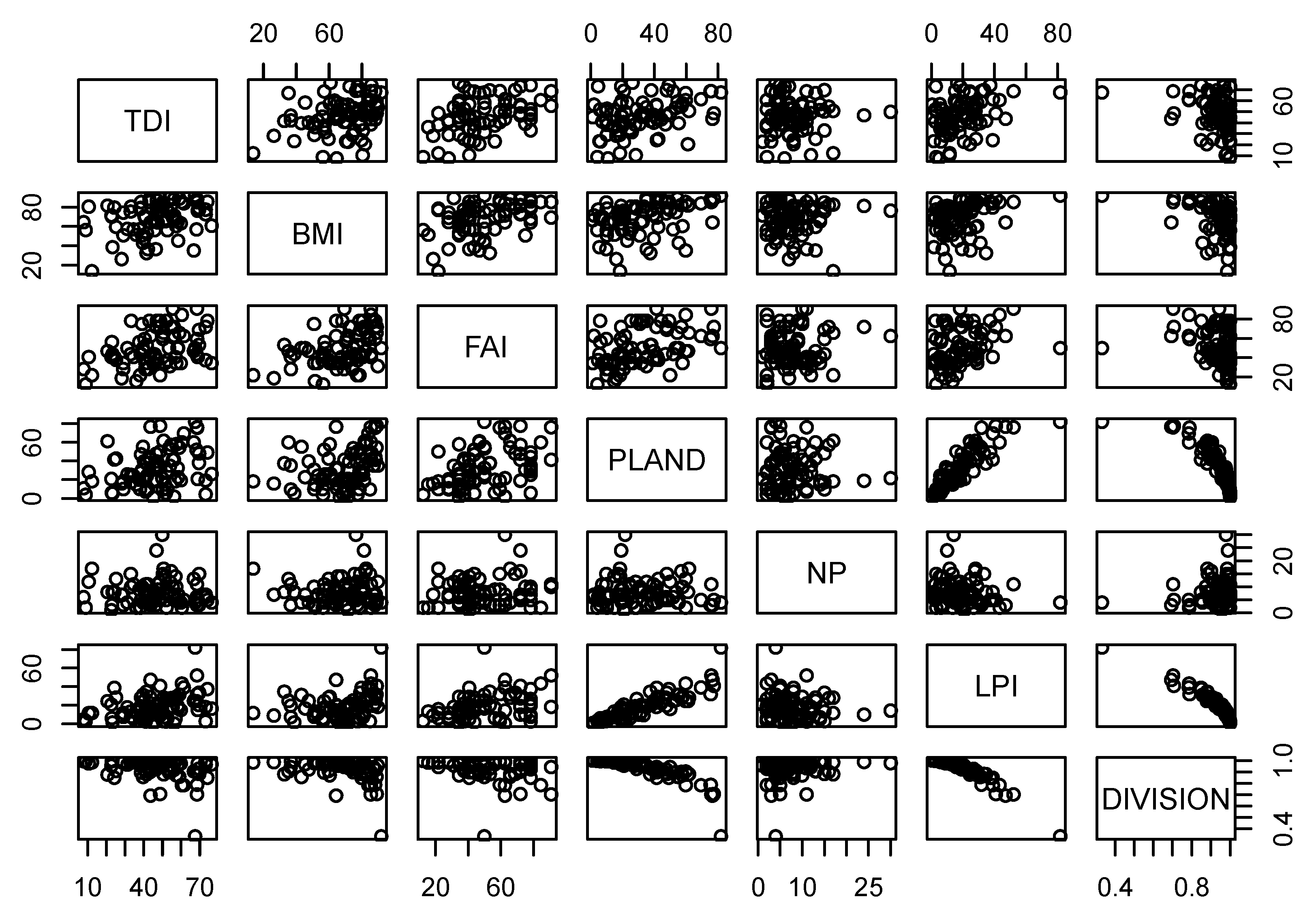
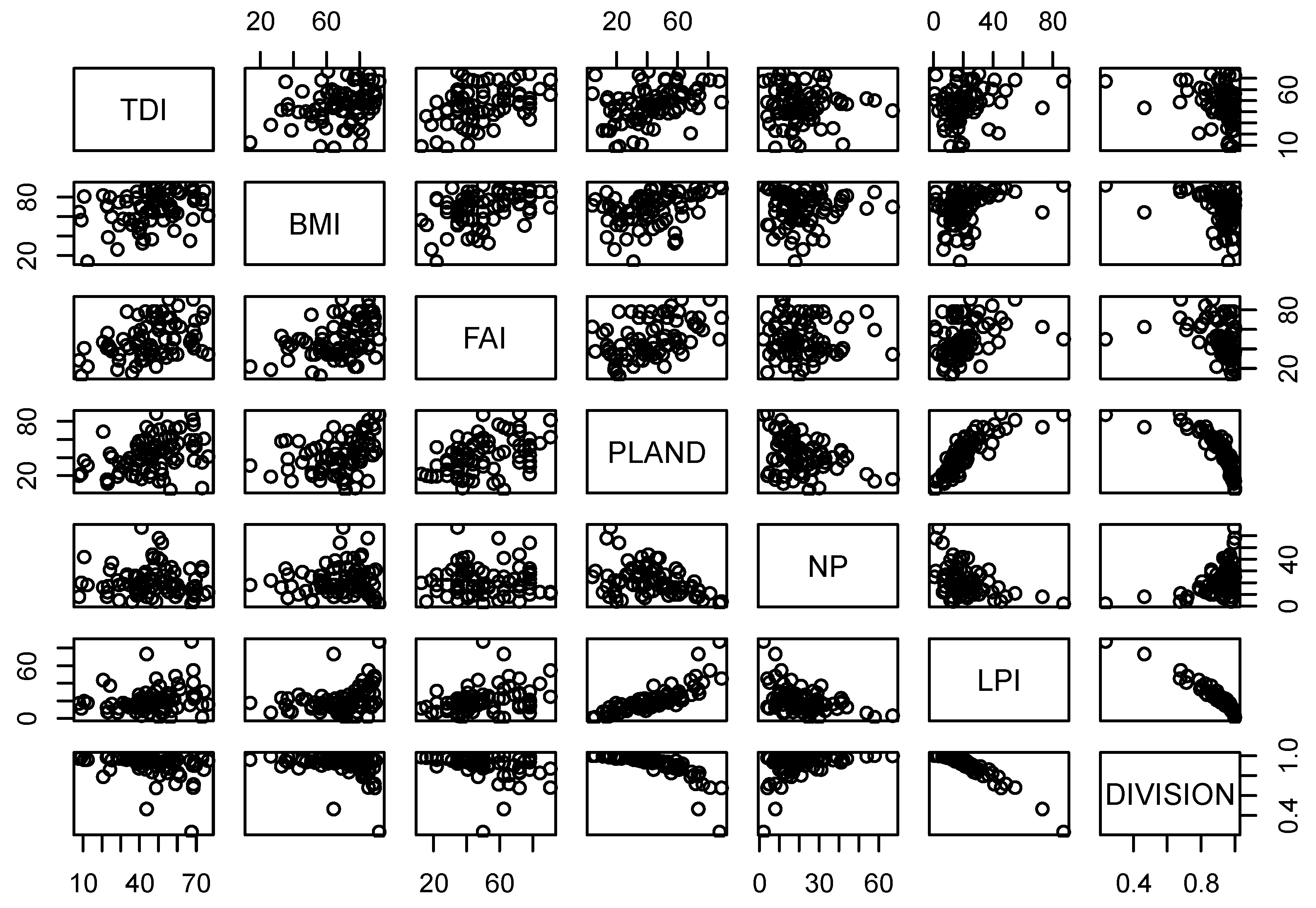
Boot resamples = 1000. * p < 0.05, ** p < 0.01. ¹⁾ Confidence level of correlation = 95%.

compares the relationships between biological indicators and forest fragmentation metrics at multiple scales. PLAND showed significant relationships with all biological indicators at all scales. Specifically, PLAND was positively correlated with TDI (r = 0.35), BMI (r = 0.40), and FAI (r = 0.43) at the 1-km riparian scale. These positive relationships of PLAND with biological indicators were consistent at 2-km and 5-km riparian scales. PLAND also showed positive relationships with TDI (r = 0.42, r = 0. 40), BMI (r = 0.42, r = 0.46) and FAI (r = 0.44, r = 0.44) at 2-km and 5-km riparian scales, respectively. Similarly, LPI showed positive correlations with TDI at 1-km (r = 0.33), 2-km (r = 0.31), and 5-km (r = 0.24) scales. We observed similar relationships between LPI and BMI at multiple scales. LPI was positively associated with BMI at 1-km (r = 0.37), 2-km (r = 0.38), and 5-km (r = 0.36) riparian scales, which was consistent with FAI at scales of 1 km (r = 0.40), 2 km (r = 0.37) and 5 km (r = 0.25). DIVISION, a negative measure of fragmentation, was significantly negatively correlated with TDI at 1-km, 2-km, and 5-km scales (r = −0.34, r = −0.35, and r = −0.29, respectively). However, DIVISION showed significant negative relationships with BMI at all riparian scales (r = −0.38, r = −0.39 and r = −0.36, respectively). Similarly, DIVISION was negatively correlated with FAI at the 1-km (r = −0.41), 2-km (r = −0.39) and 5-km (r = −0.32) scales. We also observed high variance in the confidence intervals (CI) of correlations between biological indicators and fragmentation metrics at multiple scales (Table 5). The highest upper limit of the correlation between TDI and NP was −0.5 at the 5-km scale. Similarly, the highest upper limit of the correlation between TDI and PLAND was 0.56 at the 2-km and 5-km scales. The highest correlation coefficient between TDI and LPI was observed at the 1-km scale (r = 0.5), and the strongest negative correlation between TDI and DIVISION was −0.45 at the 1-km scale. The correlations between BMI and NP showed relatively small CIs between the upper limit and lower limit compared to correlations of BMI with PLAND, LPI, or DIVISION. The highest correlation coefficients of BMI with PLAND and LPI with a 95% confidence interval were 0.56 (5-km scale) and 0.49 (2-km scale), respectively. Similarly, the strongest negative correlation between BMI and DIVISION was −0.47 at the 2-km scale. The upper limits of the correlations of FAI with PLAND and LPI were 0.59 (2- and 5-km scales) and 0.54 (1-km scale), respectively. The strongest negative correlation between FAI and DIVISION was observed at the 1-km scale (r = −0.48). A matrix of scatter plots for pairwise connections of all biological indicators and forest fragmentation metrics showed multicollinearity among variables, as shown in Figure 3 (1-km scale), Figure 4 (2-km scale) and Figure 5 (5-km scale) at the three scales analyzed. The shape and stretch of the correlations among variables indicated strong correlations (except for NP and three biological indicators, which appeared to be weakly correlated).

3.4. Variation of the Relationships over Multiplc Riparian Scales

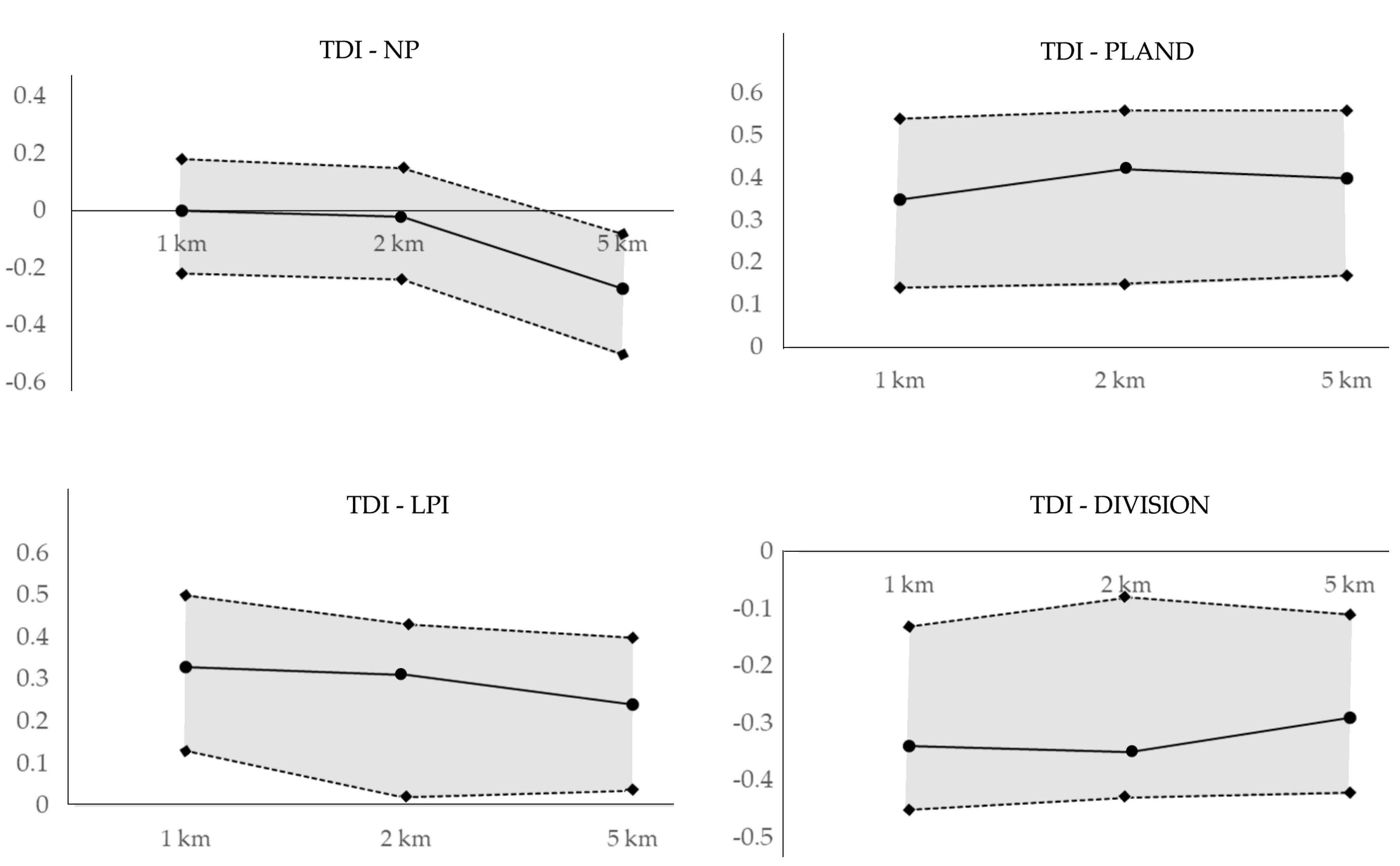
Correlations of fragmentation metrics of riparian forests with TDI (Figure 6), BMI (Figure 7), and FAI (Figure 8) revealed considerable variations in these relationships over different riparian scales. In particular, the correlation coefficients of NP with TDI were not significant at small (i.e., 1 km) and intermediate (i.e., 2 km) riparian scales, and no considerable difference was observed between correlations at small and intermediate scales. However, the correlation between NP and TDI became significant (r = −0.27) and strong at a large scale (i.e., 5 km). The CI upper and lower limits for bootstrap correlations between NP and TDI decreased significantly and in parallel, suggesting that the overall relationship between NP of riparian forest and TDI was likely stronger at a large scale than at small or intermediate scales. The relationships between PLAND and TDI at different scales showed an interesting pattern. Bootstrapped mean correlations over multiple scales fluctuated, whereas the upper and lower limits of the CI increased slightly as the observation scale increased. In contrast, the relationships between LPI and TDI, as well as the upper limits of their CIs, decreased as the observation scale increased. Thus, LPI and TDI were presumably more strongly related at a small scale than at intermediate and large riparian scales. The bootstrap mean correlation and the upper and lower limits of the CI for TDI-DIVISION were inconsistent. The mean correlation between TDI and DIVISION increased at the 5-km scale, whereas the upper limit of CI decreased at that scale.

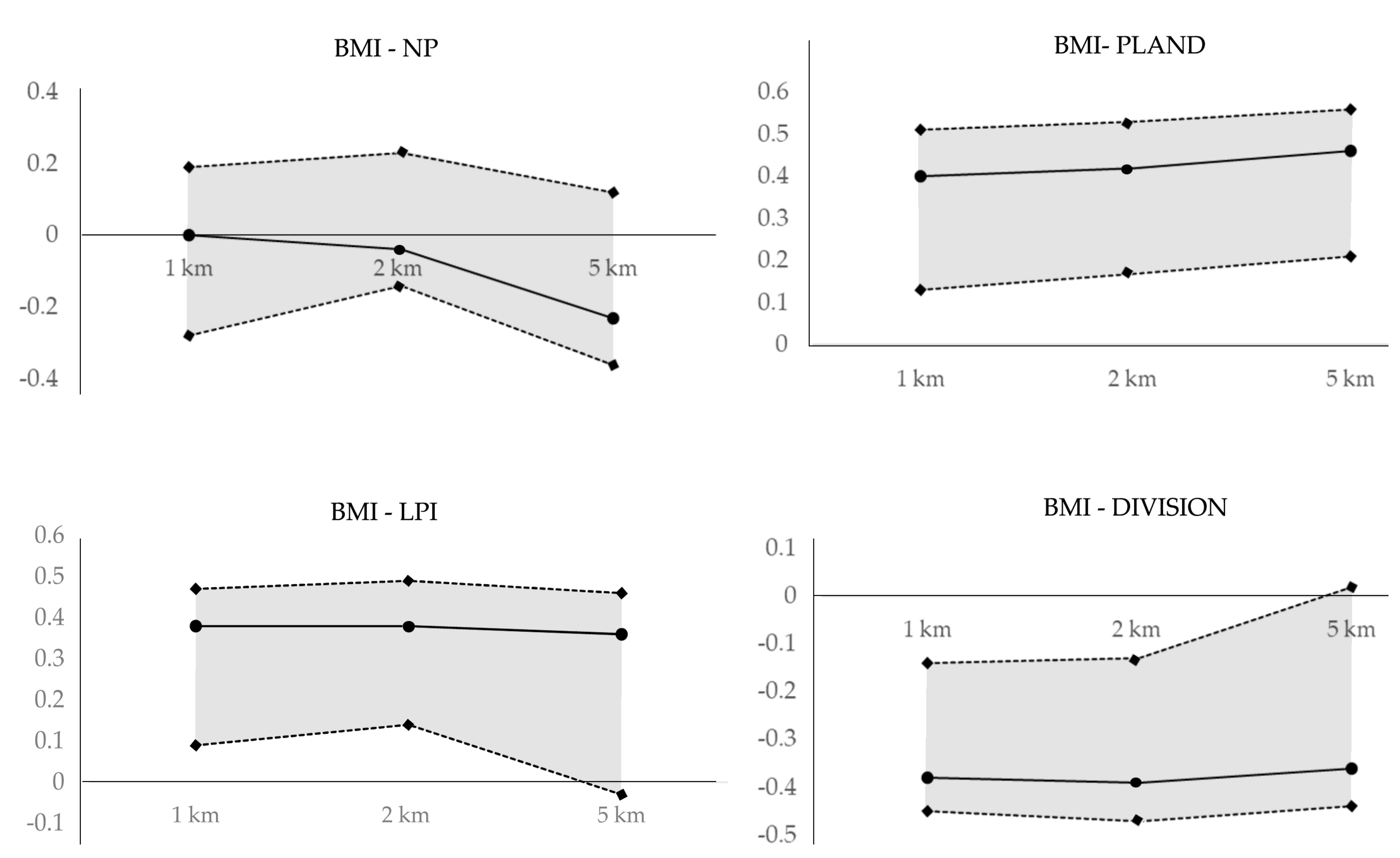
The bootstrap mean correlation and upper and lower CI limits of the relationship between NP and BMI showed somewhat complex behavior (Figure 7). The mean correlations between NP and BMI were not significant at small and intermediate scales, and the relationship decreased considerably at large scales. Meanwhile, the upper limit of CI weakened, while the lower limit of CI strengthened considerably (r = −0.36). Thus, the relationships between NP and BMI at small and intermediate scales were negligible, and these factors had a much stronger negative relationship at the large scale (i.e., 5-km scale). The mean correlations and upper and lower CI limits of the relationships between PLAND and BMI clearly showed that the relationship strengthened as the scale increased. The variance in the relationships of LPI with BMI at small and intermediate scales was minimal. Interestingly, the lower CI limit calculated at the immediate scale (r = 0.14) decreased considerably at the large scale (r = −0.03), whereas the mean correlation and the upper CI limit showed no considerable changes between the intermediate and large scales. These inconsistent variances of the mean and CI limits of the relationships between LPI and BMI among scales suggested that no considerable changes occurred in these relationships among the riparian scales tested. The relationship between DIVISION and BMI was generally the opposite of that between LPI and BMI. The mean correlation and lower CI limit weakened slightly as riparian scale increased. Meanwhile, the upper CI limit of the relationship between DIVISION and BMI at the intermediate scale (r = −0.13) changed radically, becoming a positive relationship (r = 0.02).

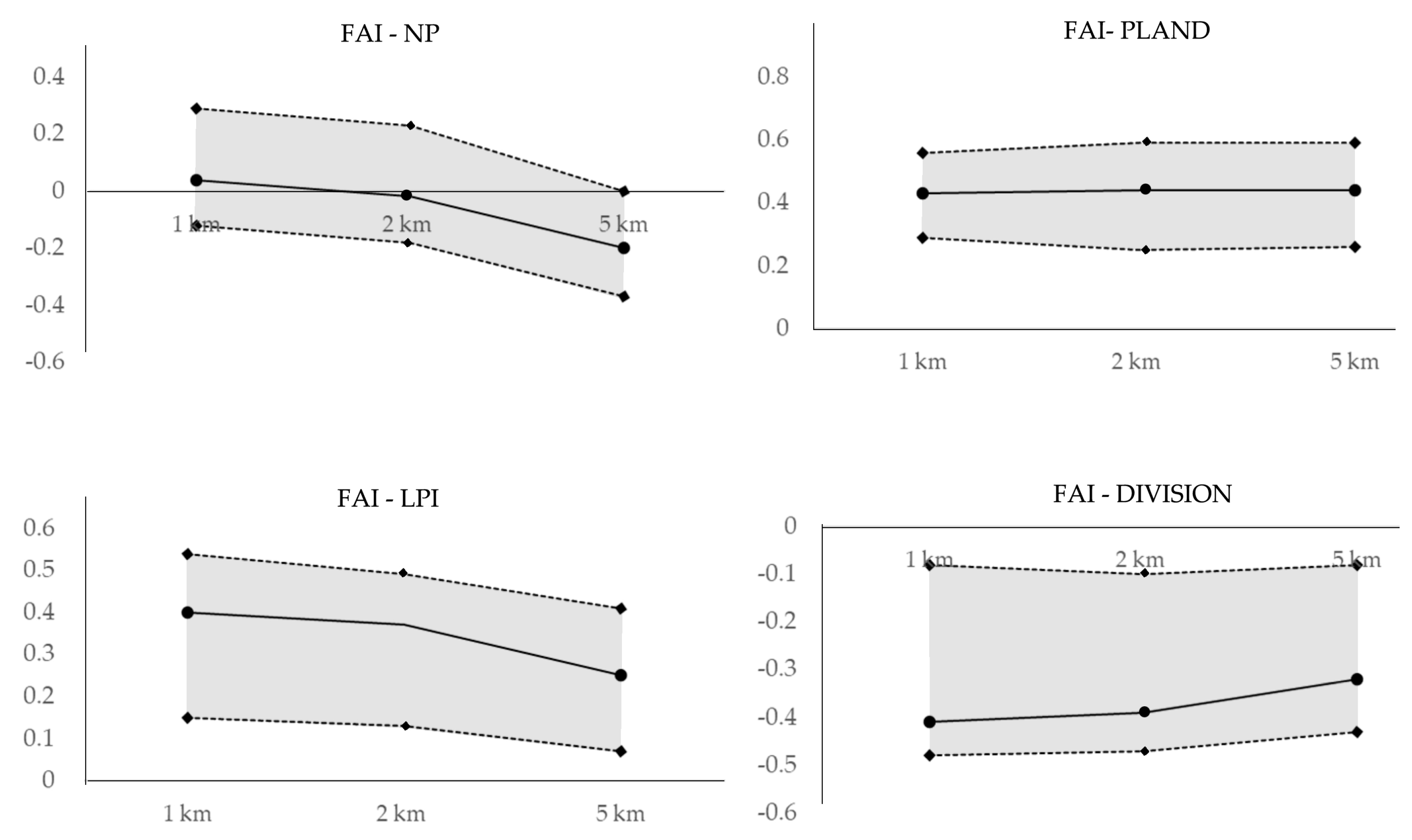
The observed relationships between NP and FAI decreased as observation scales increased (Figure 8). The bootstrap mean correlation was not significant at the small (r = 0.04) or intermediate (r = −0.02) scales (Table 5), but the relationship was much stronger at large scale. This tendency was also observed with the upper and lower CI limits of this relationship between the intermediate and large scales. Thus, the negative relationship between NP and FAI was likely stronger at large scales (i.e., 5 km) than at small (i.e., 1 km) or intermediate scales (i.e., 2 km). The bootstrap mean correlation and the upper and lower CI limits of the FAI-PLAND relationship increased slightly but consistently as riparian scale increased. In contrast, the relationship between LPI and FAI consistently decreased as riparian scale increased. Thus, the relationship between LPI and FAI was stronger at the small scale than at intermediate or large riparian scales. The bootstrap mean correlations and upper and lower CI limits of the relationships between DIVISION and FAI showed slight but consistent decreases as riparian scale increased.

Significance test using Z-score indicated that there were significant differences among correlations between fragmentation metrics and biological indicators over scales (

Table 6. Significance test using Z-score among correlations between biological indicators and fragmentation metrics over different scales.

Biological Indicators	Correlation with Variable 1	Correlation with Variable 2	Z-Score of Two Correlations	p Value
TDI	NP 1 km	NP 2 km	0.447	0.327
	NP 1 km	NP 5 km	6.182	0.00 **
	NP 2 km	NP 5 km	5.735	0.00 **
	PLAND 1 km	PLAND 2 km	−1.836	0.03 *
	PLAND 1 km	PLAND 5 km	−1.3	0.09
	PLAND 2 km	PLAND 5 km	0.537	0.29
	LPI 1 km	LPI 2 km	0.498	0.30
	LPI 1 km	LPI 5 km	−0.251	0.40
	LPI 2 km	LPI 5 km	1.692	0.04 *
	DIVISION 1 km	DIVISION 2 km	0.253	0.39
	DIVISION 1 km	DIVISION 5 km	14.572	0.00 **
	DIVISION 2 km	DIVISION 5 km	−1.493	0.05
BMI	NP 1 km	NP 2 km	0.894	0.18
	NP 1 km	NP 5 km	5.229	0.00 **
	NP 2 km	NP 5 km	4.335	0.00 **
	PLAND 1 km	PLAND 2 km	−0.537	0.29
	PLAND 1 km	PLAND 5 km	−1.645	0.05 *
	PLAND 2 km	PLAND 5 km	−1.133	0.13
	LPI 1 km	LPI 2 km	0.000	0.5
	LPI 1 km	LPI 5 km	0.517	0.30
	LPI 2 km	LPI 5 km	0.517	0.30
	DIVISION 1 km	DIVISION 2 km	0.262	0.39
	DIVISION 1 km	DIVISION 5 km	−0.517	0.30
	DIVISION 2 km	DIVISION 5 km	−0.78	0.21
FAI	NP 1 km	NP 2 km	1.34	0.09
	NP 1 km	NP 5 km	5.42	0.00 **
	NP 2 km	NP 5 km	4.8	0.00 **
	PLAND 1 km	PLAND 2 km	−0.275	0.39
	PLAND 1 km	PLAND 5 km	−1.645	0.05 *
	PLAND 2 km	PLAND 5 km	−1.108	0.13
	LPI 1 km	LPI 2 km	0.786	0.21
	LPI 1 km	LPI 5 km	3.756	0.00 **
	LPI 2 km	LPI 5 km	2.97	0.00
	DIVISION 1 km	DIVISION 2 km	−0.532	0.29
	DIVISION 1 km	DIVISION 5 km	−2.321	0.01 **
	DIVISION 2 km	DIVISION 5 km	−1.79	0.03 *

n = 79. * p < 0.05. ** p < 0.05

). In specific, the correlation between TDI and NP at large scale (i.e., 5 km) was significantly different from those small (i.e., 1 km) and (i.e., 2 km) scales. However, a significant difference in correlations was not observed between small and intermediate scales. The correlation of TDI with PLAND at small scale was significantly different from the correlation at the intermediate scale. Similarly, the correlation of TDI with LPI at intermediate scale was different from the correlation at large scale. Also, we observed that the significant differences in correlations between TDI and DIVISION were observed between large scale and small or intermediate scales. Similarly, the correlation between BMI and NP was at a large scale was significantly stronger than those at small and intermediate scales. Also, the correlation between BMI and PLAND showed a significantly stronger than the correlation at small scale. In addition, the correlation between FAI and NP was significantly different from those at a small and intermediate scales. Regarding the relationships between FAI and PLAND, we observed a significant difference in the correlation between small scale and large scale. The correlations of FAI with LPI and DIVISION at large scale was considerably weaker than those at small and intermediate scales (Table 6).

In summary, the relationships of NP with biological indicators TDI, BMI, and FAI were not significant at small and intermediate scales, but these relationships became much stronger at large scales. We also observed that the relationships between PLAND and biological indicators became stronger as riparian scale increased. Meanwhile, the relationship between LPI and biological indicators was stronger at small scales and became weaker as riparian scale increased. The strength of the negative relationship of DIVISION with biological indicators weakened as riparian scale increased. Overall, the relationships of NP and PLAND with biological indicators strengthened as riparian scale increased, whereas the relationships of LPI and DIVISION with biological indicators weakened as riparian scale increased, despite the inconsistent slopes of variances among biological indicators. Also, the variations of the relationships between biological indicators and fragmentation metrics were not consistent over different scales. Rather, the variations of the relationships over scales were dependent on the types of fragmentation metrics of riparian forest, which makes it difficult to implement the findings of this into practice.

3.5. Redundancy Analyses Variations

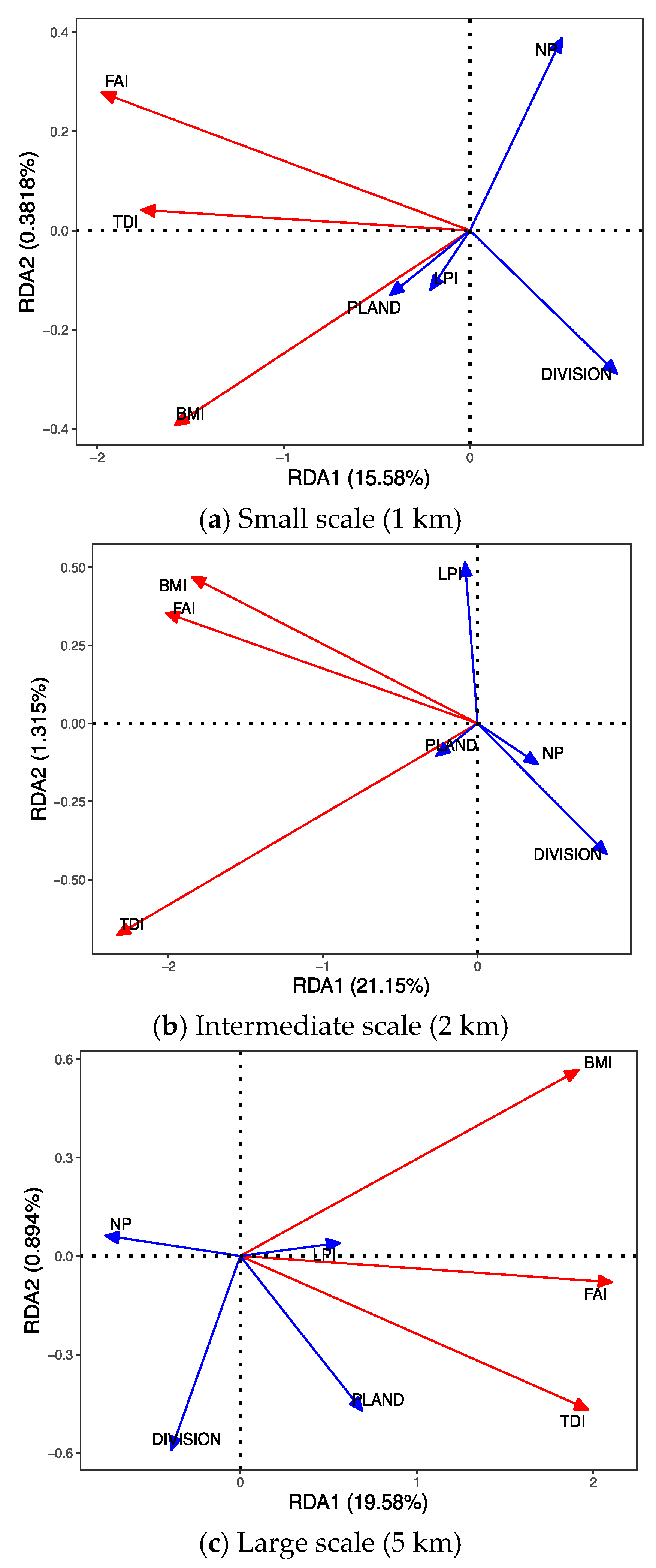
RDA revealed that the relationships among fragmentation metrics and biological indicators could be better explained at larger riparian scales. Specifically, RDA showed that DIVISION and NP had negative impacts on the biological indicators. The first two RDA axes explained all the variation in variables at the tested scales (Figure 9). Because a multitude of forest fragmentation metrics used as explanatory variables were correlated with stream biota, we assessed relationships between biological indicators and other key explanatory variables using RDA at three riparian scales. At the 1-km, 2-km, and 5-km buffer scales, forest fragmentation conditions provided an indication of biological function. RDA clearly showed that differences among the three buffer scales of forest fragmentation metrics influenced the conditions of diatoms, macroinvertebrates, and fish in streams. The forest fragmentation metrics NP and DIVISION were negatively constrained at all scales, and PLAND and LPI were positively constrained. The RDA results were found to be statistically significant (p < 0.05).

4. Discussion

Well-preserved streamside vegetation can prevent soil erosion and nutrient release into adjoining streams, as it stabilizes stream banks [116]. However, the effects of forest fragmentation on stream ecosystems have scarcely been explored [22]. In this study, we explored the relationships between riparian forest fragmentation and biological indicators, including diatom, macroinvertebrate, and fish assemblages at multiple spatial scales. Furthermore, this study examined the variance in these relationships over multiple riparian scales. According to the results of the study, communities of diatoms, macroinvertebrates, and fish measured through the biological indicators of TDI, BMI, and FAI were significantly correlated with forest fragmentation conditions calculated using the landscape metrics of the NP, PLAND, LPI, and DIVISION indices. Specifically, TDI, BMI, and FAI were positively correlated with PLAND and LPI and negatively correlated with DIVISION at all riparian scales. On the other hand, NP did not show significant relationships with any biological indicators at small (i.e., 1 km) or intermediate (i.e., 2 km) scales. However, NP was negatively correlated with biological indicators at large (i.e., 5 km) scales. The consistent positive relationships observed between PLAND and all biological indicators at multiple scales suggest that biological conditions were better when riparian forests were less fragmented at all scales. In particular, PLAND had stronger relationships with BMI than with TDI or FAI. Based on a total class area, PLAND quantifies forest composition in riparian areas, which is critical for understanding the variations in patch size [117,118] in riparian areas. These results confirmed previous findings suggesting strong positive relationships between the presence of streamside forests and biological condition [41]. These positive relationships between LPI and biological indicators indicated that the biological condition in streams was better when a large forest patch was present in the riparian area. Thus, all biological indicators were likely to improve when riparian areas were dominated by a single large forest patch. LPI is a simple measure of patch dominance in which smaller values of LPI indicate a greater degree of forest fragmentation. Previous studies have confirmed that a landscape composition dominated by a large forest is associated with better biological condition [98,119]. These results clearly showed that the FAI condition of streams was closely tied to the proximity of riparian forest patches. The closer riparian forest patches were to streams, the better the FAI condition of the streams. These results suggested that biological conditions in streams were better when riparian areas were covered with more forested area, contained larger forest patches, and the patches were located near riparian areas. These results confirmed the findings of a previous study, which suggested better biological condition with less fragmentation of riparian forests at a 500-m scale [8]. Thus, fragmentation of riparian forests was clearly negatively associated with biological condition of streams. The biological condition of a stream was generally better if riparian forests were less fragmented, regardless of riparian scale, in accordance with recent studies [1,3,8]. As discussed by Yirigui et al. (2019) and others (e.g., References [1,120]), more fragmented riparian forests may not provide the benefits of intercepting rainfall, lowering run-off speed, and increasing infiltration into soils and uptake time by plants typical of riparian areas. The results of the present study and previous findings emphasize the importance of forest fragmentation in riparian areas to the biological condition of streams and suggest that stream restoration projects should consider not only the amount of forest but also its spatial configuration in riparian areas.

Comparison of the correlations between NP and PLAND and biological indicators over multiple scales suggested that forest fragmentation at a large scale was more strongly related to biological indicators than at a small scale. Specifically, the conditions of diatoms, macroinvertebrates, and fish were more susceptible to NP and PLAND over larger areas. These results were consistent with previous studies investigating the effects of land use types and their patterns on ecological communities, which reported that protection or restoration of smaller areas was not sufficient to maintain the ecological integrity of streams [121,122]. Due to their location, streamside forests are critical to stream water quality and biological condition in many ways, including stabilization of stream banks, filtering nutrients and sediments, lowering water temperature, providing habitat, and enhancing the biodiversity of streams [2,61,62,63,123,124]. However, our results suggested that the scale and spatial pattern of forested areas might be as important for biological communities as the presence of riparian forests. Some previous studies also reported that forests in riparian areas play significant roles in the condition of diatoms, macroinvertebrates, and fish at both the watershed and riparian scales [125,126]. Broadly, larger forested areas appeared to allow maintenance of biological integrity [60,127]. However, we observed that LPI and DIVISION showed the strongest relationships with biological indicators at small scales, differing from the relationships of NP and PLAND with biological indicators. These results indicated that the effects of the presence of large riparian forest patches and the proximity of riparian forest patches might be important biological indicators in riparian areas around streams. Thus, managers and planners of river environments should consider the structure of riparian forests to mitigate the negative effects of forest fragmentation on the biological condition of streams [128,129,130].

NP did not show significant relationships with biological indicators at small (1-km) or intermediate (2-km) scales in the present study. The insignificant relationships of NP with biological indicators at small and intermediate scales may have occurred because NP was unable to quantify the degree of fragmentation at the small scale [8]. NP simply measures the number of riparian forest patches within buffer areas [95] and does not account for the degree of fragmentation or area of riparian forests at a small spatial scale, corresponding to the variation observed in biological indicators. This finding was confirmed by the relatively small standard deviation obtained at small and intermediate scales compared to that at large scale (Table 4). Another aspect of the nature of NP to consider is that NP should be high when riparian forests are severely fragmented within given buffer areas, and low when they are not fragmented. However, NP could be small (i.e., less fragmented) when only one small forest patch occurred within a riparian area. In this case, NP indicates that the riparian forests of Nakdong River are fragmented, but few forests occur in riparian areas. From this perspective, NP can be considered a conditional metric of fragmentation given the same forest area, and NP should be used cautiously when measuring fragmentation of riparian forests and interpreting such results. To make up for the shortcomings of NP, it is reasonable to use NP along with the mean size of riparian forest patches [131].

5. Conclusions

In this study, we investigated the relationships between riparian forest fragmentation and biological condition of diatoms, macroinvertebrates, and fish, and examined the variations in these relationships over multiple scales. We observed that the proportion of riparian forest (i.e., PLAND) and the largest riparian forest patch ratio (i.e., LPI) were positively correlated with biological condition of diatoms (i.e., TDI), macroinvertebrates (i.e., BMI), and fish (i.e., FAI), whereas the spatial proximity of riparian forest patches (i.e., DIVISION) showed significant negative relationships with biological indicators at multiple scales. These relationships also varied among riparian scales. Our results indicated that NP and PLAND were more important at large scales than at small scales, whereas LPI and DIVISION were more closely tied to biological indicators at small scales than at large scales. Thus, biological conditions in streams appeared better under less fragmented riparian forest conditions. Furthermore, variation in the correlations between fragmentation metrics and biological indicators over multiple scales revealed that the relationships of NP and PLAND with biological indicators became stronger as the observation scale increased, whereas LPI and DIVISION showed the opposite relationship. These results suggest that ecological communities in streams might be even more sensitive to the fragmentation of distant forests than the fragmentation of streamside forests. For river managers and planners, an ideal approach could involve restoring large riparian forest patches with high proximity among riparian forest patches in near-stream zones while maintaining more forested areas in zones that are distant from streams. These results also imply that stream corridor restoration and management that focuses on only streamside riparian forests might be insufficient for enhancing the integrity of stream ecosystems, despite numerous studies reporting positive effects of streamside riparian forests. Therefore, much larger spatial ranges of riparian forests should be considered during forest management and restoration to enhance the biological condition of streams.

References

- Alemu, T.; Bahrndorff, S.; Hundera, K.; Alemayehu, E.; Ambelu, A. Effect of riparian land use on environmental conditions and riparian vegetation in the east African highland streams. Limnologica 2017, 66, 1–11. [Google Scholar] [CrossRef]
- Anbumozhi, V.; Radhakrishnan, J.; Yamaji, E. Impact of riparian buffer zones on water quality and associated management considerations. Ecol. Eng. 2005, 24, 517–523. [Google Scholar] [CrossRef]
- Casotti, C.G.; Kiffer, W.P.; Costa, L.C.; Rangel, J.V.; Casagrande, L.C.; Moretti, M.S. Assessing the importance of riparian zones conservation for leaf decomposition in streams. Nat. Conserv. 2015, 13, 178–182. [Google Scholar] [CrossRef] [Green Version]
- Chellaiah, D.; Yule, C.M. Effect of riparian management on stream morphometry and water quality in oil palm plantations in Borneo. Limnologica 2018, 69, 72–80. [Google Scholar] [CrossRef]
- Ding, J.; Jiang, Y.; Liu, Q.; Hou, Z.; Liao, J.; Fu, L.; Peng, Q. Influences of the land use pattern on water quality in low-order streams of the Dongjiang River basin, China: A multi-scale analysis. Sci. Total Environ. 2016, 551–552, 205–216. [Google Scholar] [CrossRef] [PubMed]
- Chen, W.; Xie, X.; Wang, J.; Pradhan, B.; Hong, H.; Bui, D.T.; Duan, Z.; Ma, J. A comparative study of logistic model tree, random forest, and classification and regression tree models for spatial prediction of landslide susceptibility. Catena 2017, 151, 147–160. [Google Scholar] [CrossRef] [Green Version]
- Wang, R.; Xu, T.; Yu, L.; Zhu, J.; Li, X. Effects of land use types on surface water quality across an anthropogenic disturbance gradient in the upper reach of the Hun River, Northeast China. Environ. Monit. Assess. 2013, 185, 4141–4151. [Google Scholar] [CrossRef] [PubMed]
- Yirigui, Y.; Lee, S.W.; Nejadhashemi, A.P.; Herman, M.R.; Lee, J.W.; Yirigui, Y.; Lee, S.-W.; Nejadhashemi, A.P.; Herman, M.R.; Lee, J.-W. Relationships between Riparian Forest Fragmentation and Biological Indicators of Streams. Sustainability 2019, 11, 2870. [Google Scholar] [CrossRef]
- Zhou, T.; Wu, J.; Peng, S. Assessing the effects of landscape pattern on river water quality at multiple scales: A case study of the Dongjiang River watershed, China. Ecol. Indic. 2012, 23, 166–175. [Google Scholar] [CrossRef]
- Suga, C.M.; Tanaka, M.O. Influence of a forest remnant on macroinvertebrate communities in a degraded tropical stream. Hydrobiologia 2013, 703, 203–213. [Google Scholar] [CrossRef]
- Lee, S.W.; Hwang, S.J.; Lee, S.B.; Hwang, H.S.; Sung, H.C. Landscape ecological approach to the relationships of land use patterns in watersheds to water quality characteristics. Landsc. Urban Plan. 2009, 92, 80–89. [Google Scholar] [CrossRef]
- Midha, N.; Mathur, P.K. Assessment of forest fragmentation in the conservation priority Dudhwa landscape, India using FRAGSTATS computed class level metrics. J. Indian Soc. Remote Sens. 2010, 38, 487–500. [Google Scholar] [CrossRef]
- Bu, H.; Meng, W.; Zhang, Y.; Wan, J. Relationships between land use patterns and water quality in the Taizi River basin, China. Ecol. Indic. 2014, 41, 187–197. [Google Scholar] [CrossRef]
- Shi, P.; Zhang, Y.; Li, Z.; Li, P.; Xu, G. Influence of land use and land cover patterns on seasonal water quality at multi-spatial scales. Catena 2017, 151, 182–190. [Google Scholar] [CrossRef]
- Greenberg, L.A.; Bergman, E. Forest-Stream Linkages: Effects of Terrestrial Invertebrate Input and Light on Diet and Growth of Brown Trout (Salmo trutta) in a Boreal Forest Stream. PLoS ONE 2012, 7. [Google Scholar] [CrossRef]
- Allan, J.D.; Castillo, M.M. Stream Ecology: Structure and Function of Running Waters; Springer: Dordrecht, The Netherlands, 2007; Volume 2, ISBN 9781402055829. [Google Scholar]
- Shandas, V.; Alberti, M. Exploring the role of vegetation fragmentation on aquatic conditions: Linking upland with riparian areas in Puget Sound lowland streams. Landsc. Urban Plan. 2009, 90, 66–75. [Google Scholar] [CrossRef]
- Woznicki, S.A.; Nejadhashemi, A.P.; Tang, Y.; Wang, L. Large-scale climate change vulnerability assessment of stream health. Ecol. Indic. 2016, 69, 578–594. [Google Scholar] [CrossRef] [Green Version]
- Sowa, S.P.; Herbert, M.; Mysorekar, S.; Annis, G.M.; Hall, K.; Nejadhashemi, A.P.; Woznicki, S.A.; Wang, L.; Doran, P.J. How much conservation is enough? De fi ning implementation goals for healthy fi sh communities in agricultural rivers. J. Great Lakes Res. 2016, 42, 1302–1321. [Google Scholar] [CrossRef]
- Li, S.; Gu, S.; Tan, X.; Zhang, Q. Water quality in the upper Han River basin, China: The impacts of land use/land cover in riparian buffer zone. J. Hazard. Mater. 2009, 165, 317–324. [Google Scholar] [CrossRef]
- Liu, Y.; Wei, X.; Li, P.; Li, Q. Sensitivity of correlation structure of class- and landscape-level metrics in three diverse regions. Ecol. Indic. 2016, 64, 9–19. [Google Scholar] [CrossRef]
- Zartman, C.E.; Shaw, A.J. Metapopulation Extinction Thresholds in Rain Forest Remnants. Am. Nat. 2006, 167, 177–189. [Google Scholar] [CrossRef] [PubMed]
- Ramachandra, T.V.; Bharath, S.; Chandran, S. Geospatial analysis of forest fragmentation in Uttara Kannada District, India. For. Ecosyst. 2016, 3, 10. [Google Scholar] [CrossRef]
- Echeverria, C.; Coomes, D.A.; Hall, M.; Newton, A.C. Spatially explicit models to analyze forest loss and fragmentation between 1976 and 2020 in southern Chile. Ecol. Modell. 2008, 212, 439–449. [Google Scholar] [CrossRef]
- Snyder, M. 2015 Vermont Forest Fragmentation Report Report; Vermont Department of Forests, Parks and Recreation: Montpelier, VT, USA, 2015.
- Hunag, F.; Zhang, H.J.; Wang, P. Trajectory Analysis of Forest Changes in Northern Area of Changbai Mountains, China from Landsat Tm Image. ISPRS Int. Arch. Photogramm. Remote Sens. Spat. Inf. Sci. 2012, XXXIX-B8, 479–484. [Google Scholar] [CrossRef]
- Ramachandra, T.V.; Bharath, S. Geoinformatics based Valuation of Forest Landscape Dynamics in Central Western Ghats, India. J. Remote Sens. GIS 2018, 7, 1–8. [Google Scholar] [CrossRef]
- Davies-Colley, R.J.; Payne, G.W.; van Elswijk, M. Microforest gradients across a forest edge. N. Z. J. Ecol. 2000, 24, 111–121. [Google Scholar]
- Meleason, M.A.; Quinn, J.M. Influence of riparian buffer width on air temperature at Whangapoua Forest, Coromandel Peninsula, New Zealand. For. Ecol. Manag. 2004, 191, 365–371. [Google Scholar] [CrossRef]
- Ding, S.; Zhang, Y.; Liu, B.; Kong, W.; Meng, W. Effects of riparian land use on water quality and fish communities in the headwater stream of the Taizi River in China. Front. Environ. Sci. Eng. 2013, 7, 699–708. [Google Scholar] [CrossRef]
- Sliva, L.; Williams, D.D. Buffer Zone Versus Whole Catchment Approaches to Studying Land Use Impact on River Water Quality. Water Res. 2001, 35, 3462–3472. [Google Scholar] [CrossRef]
- de Oliveira, L.M.; Maillard, P.; de Andrade Pinto, É.J. Modeling the effect of land use/land cover on nitrogen, phosphorous and dissolved oxygen loads in the Velhas River using the concept of exclusive contribution area. Environ. Monit. Assess. 2016, 188. [Google Scholar] [CrossRef] [PubMed]
- Ou, Y.; Wang, X.; Wang, L.; Rousseau, A.N. Landscape influences on water quality in riparian buffer zone of drinking water source area, Northern China. Environ. Earth Sci. 2016, 75, 1–13. [Google Scholar] [CrossRef]
- Chang, H.; Thiers, P.; Netusil, N.R.; Yeakley, J.A.; Rollwagen-Bollens, G.; Bollens, S.M.; Singh, S. Relationships between environmental governance and water quality in a growing metropolitan area of the Pacific Northwest, USA. Hydrol. Earth Syst. Sci. 2014, 18, 1383–1395. [Google Scholar] [CrossRef] [Green Version]
- Tong, S.T.Y.; Chen, W. Modeling the relationship between land use and surface water quality. J. Environ. Manag. 2002, 66, 377–393. [Google Scholar] [CrossRef]
- Yang, H.; Wang, G.; Wang, L.; Zheng, B. Impact of land use changes on water quality in headwaters of the Three Gorges Reservoir. Environ. Sci. Pollut. Res. 2016, 23, 11448–11460. [Google Scholar] [CrossRef] [PubMed]
- Hernandez-Suarez, J.S.; Nejadhashemi, A.P. A review of macroinvertebrate—and fish—based stream health modelling techniques. Ecohydrology 2018, 11, 1–24. [Google Scholar] [CrossRef]
- Kellner, E.; Hubbart, J.A. A method for advancing understanding of streamflow and geomorphological characteristics in mixed-land-use watersheds. Sci. Total Environ. 2019, 657, 634–643. [Google Scholar] [CrossRef] [PubMed]
- Kochendorfer, J.P.; Hubbart, J.A. The roles of precipitation increases and rural land-use changes in streamflow trends in the upper Mississippi river basin. Earth Interact. 2010, 14, 1–12. [Google Scholar] [CrossRef]
- Zell, C.; Kellner, E.; Hubbart, J.A. Forested and agricultural land use impacts on subsurface floodplain storage capacity using coupled vadose zone-saturated zone modeling. Environ. Earth Sci. 2015, 74, 7215–7228. [Google Scholar] [CrossRef]
- Allan, J. Influence of land use and landscape setting on the ecological status of rivers. Limnetica 2004, 23, 187–198. [Google Scholar] [CrossRef]
- Roy, A.H.; Freeman, M.C.; Meyer, J.L.; Leigh, D.S. Patterns of Land Use Change in Upland and Riparian Areas in the Etowah River Basin. In Proceedings of the 2003 Georgia water resources conference. Institute of Ecology, University of Georgia, Athens, Georgia, USA, 23–24 April 2003; Hatcher, K.J., Ed.; 2003; pp. 1–4. [Google Scholar]
- Kim, J.A.; An, K.J.; Hwang, S.J.; Hwang, G.S.; Kim, D.O.; Kim, C.G.; Lee, S.W. Mediating effect of stream geometry on the relationship between urban land use and biological index. Paddy Water Environ. 2014, 12, 157–168. [Google Scholar] [CrossRef]
- García-Charton, J.A.; Pérez-Ruzafa, Á.; Sánchez-Jerez, P.; Bayle-Sempere, J.T.; Reñones, O.; Moreno, D. Multi-scale spatial heterogeneity, habitat structure, and the effect of marine reserves on Western Mediterranean rocky reef fish assemblages. Mar. Biol. 2004, 144, 161–182. [Google Scholar] [CrossRef]
- Liu, Z.; He, C.; Wu, J. The relationship between habitat loss and fragmentation during urbanization: An empirical evaluation from 16 world cities. PLoS ONE 2016, 11, 1–17. [Google Scholar] [CrossRef] [PubMed]
- Taylor, C.M. The shape of density dependence in fragmented landscapes explains an inverse buffer effect in a migratory songbird. Sci. Rep. 2017, 7, 1–10. [Google Scholar] [CrossRef] [PubMed]
- Reed, R.A.; Johnson-Barnard, J.; Baker, W.L. Fragmentation of a forested rocky mountain landscape, 1950–1993. Biol. Conserv. 1996, 75, 267–277. [Google Scholar] [CrossRef]
- Laurance, W.F.; Vasconcelos, H.L.; Lovejoy, T.E. Forest loss and fragmentation in the Amazon: Implications for wildlife conservation. Oryx 2000, 34, 39–45. [Google Scholar] [CrossRef]
- Li, S.; Zhao, Z.; Miaomiao, X.; Wang, Y. Investigating spatial non-stationary and scale-dependent relationships between urban surface temperature and environmental factors using geographically weighted regression. Environ. Model. Softw. 2010, 25, 1789–1800. [Google Scholar] [CrossRef]
- Turner, M.G.; O’Neill, R.V.; Gardner, R.H.; Milne, B.T. Effects of changing spatial scale on the analysis of landscape pattern. Landsc. Ecol. 1989, 3, 153–162. [Google Scholar] [CrossRef]
- de Paula, F.R.; Gerhard, P.; de Barros Ferraz, S.F.; Wenger, S.J. Multi-scale assessment of forest cover in an agricultural landscape of Southeastern Brazil: Implications for management and conservation of stream habitat and water quality. Ecol. Indic. 2018, 85, 1181–1191. [Google Scholar] [CrossRef] [Green Version]
- Park, S.R.; Lee, H.J.; Lee, S.W.; Hwang, S.J.; Byeon, M.S.; Joo, G.J.; Jeong, K.S.; Kong, D.S.; Kim, M.C. Relationships between land use and multi-dimensional characteristics of streams and rivers at two different scales. Ann. Limnol. Int. J. Lim. 2011, 47, S107–S116. [Google Scholar] [CrossRef]
- Bae, M.-J.; Kwon, Y.; Hwang, S.-J.; Chon, T.-S.; Yang, H.-J.; Kwak, I.-S.; Park, J.-H.; Ham, S.-A.; Park, Y.-S. Relationships between three major stream assemblages and their environmental factors in multiple spatial scales. Ann. Limnol. Int. J. Limnol. 2011, 47, S91–S105. [Google Scholar] [CrossRef]
- Allan, D.; Erickson, D.; Fay, J. The influence of catchment land use on stream integrity across multiple spatial scales. Freshw. Biol. 1997, 37, 149–161. [Google Scholar] [CrossRef] [Green Version]
- Fischer, J.; Lindenmayer, D.B. Landscape modification and habitat fragmentation: A synthesis. Glob. Ecol. Biogeogr. 2007, 16, 265–280. [Google Scholar] [CrossRef]
- Abell, R.; Allan, J.D. Riparian shade and stream temperatures in an agricultural catchment, Michigan, USA. SIL Proc. 1922–2010 2002, 28, 232–237. [Google Scholar] [CrossRef]
- de Mello, K.; Valente, R.A.; Randhir, T.O.; dos Santos, A.C.A.; Vettorazzi, C.A. Effects of land use and land cover on water quality of low-order streams in Southeastern Brazil: Watershed versus riparian zone. Catena 2018, 167, 130–138. [Google Scholar] [CrossRef]
- Leal, C.G.; Barlow, J.; Gardner, T.A.; Hughes, R.M.; Leitão, R.P.; Mac Nally, R.; Kaufmann, P.R.; Ferraz, S.F.B.; Zuanon, J.; de Paula, F.R.; et al. Is environmental legislation conserving tropical stream faunas? A large-scale assessment of local, riparian and catchment-scale influences on Amazonian fish. J. Appl. Ecol. 2018, 55, 1312–1326. [Google Scholar] [CrossRef]
- Berges, S.A. Ecosystem services of riparian areas: Stream bank stability and avian habitat. Master’s Thesis, Iowa State University, Ames, IA, USA, 2009. [Google Scholar]
- Allan, J.D. Landscapes and Riverscapes: The Influence of Land Use on Stream Ecosystems. Annu. Rev. Ecol. Evol. Syst. 2004, 35, 257–284. [Google Scholar] [CrossRef] [Green Version]
- Rankins, A.; Shaw, D.R.; Boyette, M.; Rankins, A.; Shaw, D.R. Perennial Grass Filter Strips for Reducing Herbicide Losses in Runoff. Weed Sci. 2001, 49, 647–651. [Google Scholar] [CrossRef]
- Brooks, R.T.; Nislow, K.H.; Lowe, W.H.; Wilson, M.K.; King, D.I. Forest succession and terrestrial-aquatic biodiversity in small forested watersheds: A review of principles, relationships and implications for management. Forestry 2012, 85, 315–327. [Google Scholar] [CrossRef]
- Fernandes, M.R.; Aguiar, F.C.; Ferreira, M.T. Assessing riparian vegetation structure and the influence of land use using landscape metrics and geostatistical tools. Landsc. Urban Plan. 2011, 99, 166–177. [Google Scholar] [CrossRef] [Green Version]
- Broadmeadow, S.B.; Nisbet, T.R. The effects of riparian forest management on the freshwater environment: A literature review of best management practice. Hydrol. Earth Syst. Sci. 2004, 8, 286–305. [Google Scholar] [CrossRef]
- He, C.; Malcolm, S.B.; Dahlberg, K.A.; Fu, B. A conceptual framework for integrating hydrological and biological indicators into watershed management. Landsc. Urban Plan. 2000, 49, 25–34. [Google Scholar] [CrossRef]
- Naiman, R.J.; De’camps, H.; McClain, M.E. Riparia—Ecology, Conservation and Management of Streamside Communities; Elsevier Academic Press: London, UK, 2005; ISBN 0126633150. [Google Scholar]
- Turner, M.G. Landscape Ecology: The Effect of Pattern on Process. Annu. Rev. Ecol. Syst. 1989, 20, 171–197. [Google Scholar] [CrossRef]
- Tanaka, M.O.; de Fernandes, J.F.; Suga, C.M.; Hanai, F.Y.; de Souza, A.L.T. Abrupt change of a stream ecosystem function along a sugarcane-forest transition: Integrating riparian and in-stream characteristics. Agric. Ecosyst. Environ. 2015, 207, 171–177. [Google Scholar] [CrossRef]
- Hering, D.; Johnson, R.K.; Kramm, S.; Schmutz, S.; Szoszkiewicz, K.; Verdonschot, P.F.M. Assessment of European streams with diatoms, macrophytes, macroinvertebrates and fish: A comparative metric-based analysis of organism response to stress. Freshw. Biol. 2006, 51, 1757–1785. [Google Scholar] [CrossRef]
- Hwang, S.J.; Kim, N.Y.; Won, D.H.; An, K.G.; Lee, J.K.; Kim, C.S. Biological assessment of water quality by using epilithic diatoms in major river systems (Geum, Youngsan, Seomjin River), Korea. J. Korean Soc. Water Qual. 2006, 22, 784–795. (In Korean) [Google Scholar]
- Bae, M.J.; Li, F.; Kwon, Y.S.; Chung, N.; Choi, H.; Hwang, S.J.; Park, Y.S. Concordance of diatom, macroinvertebrate and fish assemblages in streams at nested spatial scales: Implications for ecological integrity. Ecol. Indic. 2014, 47, 89–101. [Google Scholar] [CrossRef]
- Beyene, A.; Addis, T.; Kifle, D.; Legesse, W.; Kloos, H.; Triest, L. Comparative study of diatoms and macroinvertebrates as indicators of severe water pollution: Case study of the Kebena and Akaki rivers in Addis Ababa, Ethiopia. Ecol. Indic. 2009, 9, 381–392. [Google Scholar] [CrossRef]
- Delgado, C.; Pardo, I.; García, L. Diatom communities as indicators of ecological status in Mediterranean temporary streams (Balearic Islands, Spain). Ecol. Indic. 2012, 15, 131–139. [Google Scholar] [CrossRef]
- Kelly, M.G.; Whitton, B.A. The Trophic Diatom Index: A new index for monitoring eutrophication in rivers. J. Appl. Phycol. 1995, 7, 433–444. [Google Scholar] [CrossRef]
- Herman, M.R.; Nejadhashemi, A.P. A review of macroinvertebrate- and fish-based stream health indices. Ecohydrol. Hydrobiol. 2015, 15, 53–67. [Google Scholar] [CrossRef] [Green Version]
- Eum, H.; Simonovic, S.P. Integrated Reservoir Management System for Adaptation to Climate Change: The Nakdong River Basin in Korea. Water Resour. Manag. 2010, 24, 3397–3417. [Google Scholar] [CrossRef]
- Lee, J.H.; Han, J.H.; Kumar, H.K.; Choi, J.K.; Byeon, H.K.; Choi, J.; Kim, J.K.; Jang, M.H.; Park, H.K.; An, K.G. National-level integrative ecological health assessments based on the index of biological integrity, water quality, and qualitative habitat evaluation index, in Korean rivers. Ann. Limnol. Int. J. Limnol. 2011, 47, S73–S89. [Google Scholar] [CrossRef]
- Bae, Y.J.; Kil, H.K.; Bae, K.S. Benthic macroinvertebrates for uses in stream biomonitoring and restoration. KSCE J. Civ. Eng. 2005, 9, 55–63. [Google Scholar] [CrossRef]
- Jun, Y.C.; Won, D.H.; Lee, S.H.; Kong, D.S.; Hwang, S.J. A multimetric benthic macroinvertebrate index for the assessment of stream biotic integrity in Korea. Int. J. Environ. Res. Public Health 2012, 9, 3599–3628. [Google Scholar] [CrossRef] [PubMed]
- Belton, T.J.; Ponader, K.; Charles, D.F. Trophic diatom indices (TDI) and the development of site-specific nutrient criteria. Proc. Water Environ. Fed. 2005, 1042–1056. [Google Scholar] [CrossRef]
- Shen, R.; Ren, H.; Yu, P.; You, Q.; Pang, W.; Wang, Q. Benthic diatoms of the Ying River (Huaihe river basin, China) and their application in water trophic status assessment. Water 2018, 10, 1013. [Google Scholar] [CrossRef]
- Shilling, F. California Watershed Assessment Manual, Volume II: Benthic Macroinvertebrates as Indicators of Watershed Condition. 2006. Available online: http://cwam.ucdavis.edu/Volume_2/TOC.htm (accessed on 13 August 2019).
- Loogen, F.; Kreuzer, H. Prevention and early diagnosis of heart and coronary diseases. Lebensversicher. Med. 1975, 27, 107–114. [Google Scholar] [PubMed]
- Stribling, J.B.; Dressing, S.A. Technical Memorandum #4: Applying Benthic Macroinvertebrate Multimetric Indexes to Stream Condition Assessments; United States Environmental Protection Agency: Washington, DC, USA, 2015; p. 14.
- Karr, J.R.; Fausch, K.D.; Angermeier, P.L.; Yant, P.R.; Schlosser, I.J. Assessing biological integrity in running waters: A method and its rationale; Illinois Natural History Survey Special Publication 5; Developed for U.S. Environmental Protection Agency by Tetra Tech, Inc.: Fairfax, VA, USA, 1986; p. 9. [Google Scholar]
- Ahn, C.H.; Joo, J.C.; Kwon, J.H.; Song, H.M. Evaluation on Functional Assessment for Fish Habitat of Underground type Eco-Artificial Fish Reef using the Index of Biological Integrity (IBI) and Qualitative Habitat Evaluation Index (QHEI). Korean Soc. Civ. Eng. 2011, 31, 565–575. [Google Scholar]
- MOE/NIER. Survey and Evaluation of Aquatic Ecosystem Health in Korea; MOE/NIER: Incheon, Korea, 2012. (In Korean) [Google Scholar]
- Heartsill-Scalley, T.; Aide, T.M. Riparian Vegetation and Stream Condition in a Tropical Agriculture-Secondary Forest Mosaic. Ecol. Appl. 2003, 13, 225–234. [Google Scholar] [CrossRef]
- King, R.S.; Baker, M.E.; Whigham, D.F.; Weller, D.E.; Jordan, T.E.; Kazyak, P.F.; Hurd, M.K. Spatial Considerations for Linking Watershed Land Cover to Ecological Indicators in Streams. Ecol. Appl. 2005, 15, 137–153. [Google Scholar] [CrossRef]
- Poiani, K.A.; Richter, B.D.; Anderson, M.G.; Richter, H.E. Biodiversity Conservation at Multiple Scales: Functional Sites, Landscapes, and Networks. Bioscience 2000, 50, 133. [Google Scholar] [CrossRef]
- Lausch, A.; Herzog, F. Applicability of landscape metrics for the monitoring of landscape change: Issues of scale, resolution and interpretability. Ecol. Indic. 2002, 2, 3–15. [Google Scholar] [CrossRef]
- Peng, J.; Wang, Y.; Zhang, Y.; Wu, J.; Li, W.; Li, Y. Evaluating the effectiveness of landscape metrics in quantifying spatial patterns. Ecol. Indic. 2010, 10, 217–223. [Google Scholar] [CrossRef]
- Hwang, S.A.; Hwang, S.J.; Park, S.R.; Lee, S.W. Examining the Relationships between Watershed Urban Land Use and Stream Water Quality Using Linear and Generalized Additive Models. Water 2016, 8, 155. [Google Scholar] [CrossRef]
- McGarigal, K. FRAGSTATS 4 Tutorial. 2015. Available online: http://planet.botany.uwc.ac.za/nisl/BCB_BIM_honours/Fragmentation/tutorial/Tutorial/tutorial.pdf (accessed on 13 August 2019).
- Mcgarigal, K. Landscape Pattern Metrics; Wiley Online Library: Hoboken, NJ, USA, 2014. [Google Scholar] [CrossRef]
- Batistella, M.; Robeson, S.; Moran, E.F. Settlement Design, Forest Fragmentation, and Landscape Change in Rondônia, Amazônia. Photogramm. Eng. Remote Sens. 2003, 69, 805–812. [Google Scholar] [CrossRef]
- Frate, L.; Carranza, M. Quantifying Landscape-Scale Patterns of Temperate Forests over Time by Means of Neutral Simulation Models. ISPRS Int. J. Geo Inf. 2013, 2, 94–109. [Google Scholar] [CrossRef]
- Looze, B.E. Forest Fragmentation Patterns in Maine Watersheds and Prediction of Visible Crown Diameter in Recent Undisturbed Forest. Master’s Thesis, University of Wisconsin, Madison, Wisconsin, 2009. [Google Scholar]
- Tolessa, T.; Senbeta, F.; Kidane, M. Landscape composition and configuration in the central highlands of Ethiopia. Ecol. Evol. 2016, 6, 7409–7421. [Google Scholar] [CrossRef] [PubMed]
- McGarigal, K.; Cushman, S.A.; Ene, E. FRAGSTATS v4: Spatial Pattern Analysis Program for Categorical and Continuous Maps. 2012. Available online: http://www.umass.edu/landeco/research/fragstats/fragstats.html (accessed on 13 August 2019).
- Kim, H.Y. Statistical notes for clinical researchers: assessing normal distribution (2) using skewness and kurtosis. Restor. Dent. Endod. 2013, 38, 52–54. [Google Scholar] [CrossRef] [PubMed]
- Ghasemi, A.; Zahediasl, S. Normality Tests for Statistical Analysis: A Guide for Non-Statisticians. Int. J. Endocrinol. Metab. 2012, 10, 486–489. [Google Scholar] [CrossRef] [PubMed] [Green Version]
- Davison, A.C.; Kuonen, D. An Introduction to the Bootstrap with Applications in R. Stat. Comput. Stat. Graph. Newsl. 2003, 13, 1–7. [Google Scholar]
- Davison, A.C.; Hinkley, D.V. Bootstrap Methods and their Application; Cambridge University Press: New York, NY, USA, 1997. [Google Scholar]
- Efron, B.; Tibshirani, R. Bootstrap Methods for Standard Errors, Confidence Intervals, and Other Measures of Statistical Accuracy. Stat. Sci. 1986, 1, 54–75. [Google Scholar] [CrossRef]
- Ames, D.P.; Asce, M. Estimating 7Q10 Confidence Limits from Data: A Bootstrap Approach. J. Water Resour. Plan. Manag. 2006, 132, 204–208. [Google Scholar] [CrossRef]
- Ide, J.; Chiwa, M.; Higashi, N.; Maruno, R.; Mori, Y.; Otsuki, K. Determining storm sampling requirements for improving precision of annual load estimates of nutrients from a small forested watershed. Environ. Monit Assess 2012, 184, 4747–4762. [Google Scholar] [CrossRef]
- Vigiak, O.; Bende-Michl, U. Estimating bootstrap and Bayesian prediction intervals for constituent load rating curves. Water Resour. Res. 2013, 49, 8565–8578. [Google Scholar] [CrossRef] [Green Version]
- Darken, P.F.; Zipper, C.E.; Holtzman, G.I.; Smith, E.P. Serial correlation in water quality variables: Estimation and implications for trend analysis. Water Resour. Res. 2002, 38, 1–7. [Google Scholar] [CrossRef]
- Darken, P.F.; Holtzman, G.I.; Smith, E.P.; Zipper, C.E. Detecting changes in trends in water quality using modified Kendall’s tau. Environmetrics 2000, 11, 423–434. [Google Scholar]
- Xing, L.; Liu, H.; Zhang, X.; Hecker, M. A comparison of statistical methods for deriving freshwater quality criteria for the protection of aquatic organisms. Environ. Sci. Pollut. Res. 2014, 21, 159–167. [Google Scholar] [CrossRef] [PubMed]
- Cohen, J.; Cohen, P.; West, S.G.; Aiken, L.S. Applied Multiple Regression/Correlation Analysis for the Behavioral Sciences, 3rd ed.; Psychology Press: New York, NY, USA, 2003. [Google Scholar]
- Oksanen, J. Unconstrained Ordination: Tutorial with R and Vegan. R Package Vegan. 2012. Available online: http://cc.oulu.fi/~jarioksa/opetus/metodi/sessio1res.pdf (accessed on 13 August 2019).
- Borcard, D.; Gillet, F.; Legendre, P. Numerical Ecology with R, 2nd ed.; Springer: New York, NY, USA, 2011; ISBN 0123266505. [Google Scholar]
- Emilson, C.E.; Canada, N.R.; Kreutzweiser, D.P.; Canada, N.R.; Gunn, J.M.; Mykytczuk, N.C.S. Leaf-litter microbial communities in boreal streams linked to forest and wetland sources of dissolved organic carbon. Ecosphere 2017, 8, 1–13. [Google Scholar] [CrossRef]
- Osborne, L.L.; Kovacic, D.A. Riparian begetated buffer strips in water-quality restoration and stream management. Freshw. Biol. 1993, 29, 243–258. [Google Scholar] [CrossRef]
- Rachel, R.; Andrew, L.; Michael, H.; Tonya, L. Fragmentation Statistics for FIA: Designing an Approach. In Proceedings of the Third Annual Forest Inventory and Analysis Symposium, Traverse City, MI, USA, 17–19 October 2001; McRoberts, R.E., Reams, G.A., Van Deusen, P.C., Moser, J.W., Eds.; 2002; pp. 146–155. [Google Scholar]
- Gerald, E.; James, R.; Nicholas, C.; Dominick, A. Forest fragmentation of the conterminous United States: Assessing forest intactness through road. Bioscience 2002, 52, 411–422. [Google Scholar]
- Alberti, M.; Booth, D.; Hill, K.; Coburn, B.; Avolio, C.; Coe, S.; Spirandelli, D. The impact of urban patterns on aquatic ecosystems: An empirical analysis in Puget lowland sub-basins. Landsc. Urban Plan. 2007, 80, 345–361. [Google Scholar] [CrossRef]
- Gharabaghi, B.; Rudra, R.P.; Whiteley, H.R.; Dickinson, W.T. Development of a management tool for vegetative filter strips. J. Water Manag. Model. 2002, 289–302. [Google Scholar] [CrossRef]
- Roth, N.E.; Allan, J.D.; Erickson, D.L. Landscape influences on steram biotic integrity assessed at multiple spatial scales. Landsc. Ecol. 1996, 11, 141–156. [Google Scholar] [CrossRef]
- Wang, L.; Lyons, J.; Kanehl, P.; Gatti, R. Influence of Watershed Land Use on Habitat Quality and Biotic Integrity in Wisconsin Streams. Fisheries 1997, 22, 6–12. [Google Scholar] [CrossRef]
- Jun, Y.C.; Kim, N.; Kwon, S.J.; Han, S.C.; Hwang, I.C.; Park, J.H.; Won, D.H.; Byun, M.S.; Kong, H.Y.; Lee, J.E.; et al. Effects of land use on benthic macroinvertebrate communities: Comparison of two mountain streams in Korea. Ann. Limnol. Int. J. Limnol. 2011, 47, S35–S49. [Google Scholar] [CrossRef] [Green Version]
- Pusey, B.J.; Arthington, A.H. Importance of the riparian zone to the conservation and management of freshwater fish: A review. Mar. Freshw. Res. 2003, 54, 1–16. [Google Scholar] [CrossRef]
- Blinn, D.W.; Bailey, P.C.E. Land-use influence on stream water quality and diatom communities in Victoria, Australia: A response to secondary salinization. Hydrobiologia 2001, 466, 231–244. [Google Scholar] [CrossRef]
- Stewart, J.S.; Wang, L.; Lyons, J.; Horwatich, J.A.; Bannerman, R. Influences of Watershed, Riparian-Corridor, and Reach-Scale Characteristics on Aquatic Biota in Agricultural Watersheds. J. Am. Water Resour. Assoc. 2001, 37, 1475–1487. [Google Scholar] [CrossRef]
- Jansirani, D.; Karthick Raja, N.; Hariprasanth, R.J.; Sweetin Preethi, S.; Sorna Kumar, R.S.A. Synthesis of colloidal starched silver nanoparticles by sonochemical method and evaluation of its antibacterial activity. J. Chem. Pharm. Sci. 2016, 9, 177–179. [Google Scholar] [CrossRef]
- Mcintyre, A.S.; Barrett, G.W.; Biology, S.C.; Mar, N.; Mcintyre, S. Habitat Variegation, An Alternative to Fragmentation. Conserv. Biol. 1992, 6, 146–147. [Google Scholar] [CrossRef]
- Kothawala, D.N.; Ji, X.; Laudon, H.; Ågren, A.M.; Futter, M.N.; Köhler, S.J.; Tranvik, L.J. The relative influence of land cover, hydrology, and in-stream processing on the composition of dissolved organic matter in boreal streams. J. Geophys. Res. G Biogeosc. 2015, 120, 1491–1505. [Google Scholar] [CrossRef]
- Brogna, D.; Vincke, C.; Brostaux, Y.; Soyeurt, H.; Dufrêne, M.; Dendoncker, N. How does forest cover impact water flows and ecosystem services? Insights from “real-life” catchments in Wallonia (Belgium). Ecol. Indic. 2017, 72, 675–685. [Google Scholar] [CrossRef]
- McGarial, K.; Marks, B. Fragstats: Spatial Pattern Analysis Program for Quantifying Landscape Structure; U.S. Department of Agriculture, Forest Service, Pacific Northwest Research Station: Portland, OR, USA, 1995; 122p.
Figure 1.
Distribution of monitoring sites in the Nakdong River system.
Figure 2.
Examples of fragmentation metrics with conceptual diagrams of riparian vegetation.
Figure 3.
Scatter plots of biological indicators and fragmentation metrics at 1 km scale.
Figure 4.
Scatter plots of biological indicators and fragmentation metrics at 2 km scale.
Figure 5.
Scatter plots of biological indicators and fragmentation metrics at 5 km scale.
Figure 6.
Variation in the correlations between fragmentation metrics and trophic diatom index (TDI) at different scales. Continuous lines represent the mean bootstrap correlations and dashed lines are the upper and lower limits of the confidence interval (95% level).
Figure 7.
Variation in the correlations between fragmentation metrics and benthic macroinvertebrates index (BMI) at different scales. Continuous lines represent the mean bootstrap correlations and dashed lines are the upper and lower limits of the confidence interval (95% level).
Figure 8.
Variation in the correlations between fragmentation metrics and fish assessment index (FAI) at different scales. Continuous lines represent the mean bootstrap correlations and dashed lines are the upper and lower limits of the confidence interval (95% level).
Figure 9.
Redundancy analysis showing associations between stream biological indicators and forest fragmentation metrics.