The Application of Improved SWAT Model to Hydrological Cycle Study in Karst Area of South China

1
School of Water Resources and Environment, China University of Geosciences (Beijing), Beijing 100083, China
2
Institute of Karst Geology, Chinese Academy of Geological Sciences, Guilin 541000, China
*
Author to whom correspondence should be addressed.
Sustainability 2019, 11(18), 5024; https://doi.org/10.3390/su11185024
Submission received: 3 August 2019
/
Revised: 21 August 2019
/
Accepted: 9 September 2019
/
Published: 13 September 2019
(This article belongs to the Section Environmental Sustainability and Applications)
Abstract
:In the karst area of southern China, karst water is important for supporting the sustainable production and home living for the local residents. Consequently, it is of significance to fully understand the water cycle, so as to make full use of water resources. In karst areas, epikarst and conduits are developed, participating in the hydrological cycle actively. For conventional lumped hydrologic models, it is difficult to simulate the hydrological cycle accurately. These models neglect to consider the variation of underlying surface and weather change. Meanwhile, for the original distributed hydrological model, the existence of epikarst and underground conduits as well as inadequate data information also make it difficult to achieve accurate simulation. To this end, the framework combining the advantages of lumped model–reservoir model and distributed hydrologic model–Soil and Water Assessment Tool (SWAT) model is established to simulate the water cycle efficiently in a karst area. Xianghualing karst watershed in southern China was selected as the study area and the improved SWAT model was used to simulate the water cycle. Results show that the indicators of ENS and R2 in the calibration and verification periods are both above 0.8, which is evidently improved in comparison with the original model. The improved SWAT model is verified to have better efficiency in describing the hydrological cycle in a typical karst area.
1. Introduction
In the karst area of south China, the complexity of karst morphological structure and inhomogeneity of karst spatial distribution bring great difficulty to water resource exploration, evaluation and development. In comparison with other areas, the high-permeability of karst structure makes underground runoff more abundant than surface runoff. So, the water cycle in karst areas is distinct compared with non-karst areas [1]. In the process of karst water resource evaluation, problems of inadequate long-term observation data and difficulty in acquiring the karst aquifer media structure and hydraulic parameters often emerge [2]. The watershed hydrological model has played an important role in many respects, such as hydrological cycle process simulation, water resources assessment and forecast, flood forecast, water conservancy project planning and design and so on. The commonly used watershed hydrological models are lumped hydrological model and distributed hydrological model.
The lumped hydrological model usually generalizes the hydrological processes, the input variable and the boundary condition. The advantages of this type of model are summarized as relatively low data requirement and convenient computation. However, the shortcoming of the model is also obvious. The lumped hydrological model is incapable of considering the spatial variation of underlying surface, which in karst areas are more prominent. So, the application of the lumped model to this kind of area is limited. In recent years, numerous trials and improvements have been conducted to make the lumped watershed hydrological model applicable to karst basins [3]. Based on the conceptual model of hydrologic behavior in a karst system, the lumped model usually has three types, summarized as the one reservoir model, two reservoirs model and three reservoirs model. For the one reservoir model, it is assumed that the whole discharge of the karst system obeys Maillet’s Law. For example, in order to simulate discharge and volume in a systemic way, only the one reservoir model was used to represent both the saturated and unsaturated zone of Lez karst aquifer in the South of France [4]. The advantage of this type of model is that the model with very few parameters is simple to construct and calculate and it is not quite sensitive to over-parameterization. The disadvantages of the one reservoir model are that the model cannot simulate the hydrologic behavior of different parts in a karst system with detail and the assumption that the whole discharge obeys Maillet’s Law is not quite realistic in a karst system. As for the two reservoirs model, an upper (faster) and a lower (slower) reservoir were used to represent the two different karstic formations respectively [5]. For example, the two reservoirs model was used to simulate the hydrology, sediment transport and nutrient loads of Krathis river basin [6]. Nikolaidis et al. (2013) have coupled the two reservoirs model (upper and lower reservoirs) with a SWAT model [7]. This kind of model considers the flow in fracture and conduit of karst aquifers and simulates hydrologic behavior in a more detailed way in comparison with the one reservoir model; however, they ignore the function of epikarst. Zhou et al. (2019) proposed a coupled lumped model called K-XAJ with two reservoirs for simulating runoff in both the karst and non-karst area, and the model produced better forecasts than the traditional XAJ (Xinanjiang) model [8]. Zhao et al. (2019) proposed the improved Xin’anjiang Model (IXAJ) by adding the regulation of ground runoff and integrating conduit flow, surface water, and groundwater into total runoff [9]. However, both the K-XAJ and IXAJ models did not consider the influence of land use type, land slope and climate change. In this paper, we used the three reservoirs model which equivalently replaced epikarst, underground conduit and micro-fissure systems. Although this kind of three reservoirs model has been used [10], few have coupled it with distributed hydrological models. In this paper, we tried to couple the three reservoirs model with the distributed model-SWAT. The hypothesis of the three reservoirs model is more realistic in karst aquifer modeling compared with the other two, and the SWAT model can consider the influence of land use type, soil type, land slope, epikarst, quick flow in conduits, slow flow in micro-fracture, climate change and so on. Through coupling the lumped model with the distributed model, the whole hydrological cycle process including the surface flow and underground flow can be sufficiently simulated.
Compared with the lumped hydrological model, the distributed hydrological model describes the spatial and temporal variations in a more detail way. It can reflect the influence of human activity on hydrological processes and fully consider the spatial variation of watershed underlying surface and the temporal variation of meteorological conditions; consequently, the model parameters have relatively clear physical meanings. Therefore, it can accurately simulate the hydrological process and make hydrologic information coincide with the actual situation. Nevertheless, this kind of model also has the weaknesses that it needs a lot of basic data and is difficult to set up. Moreover, there are poor information data, even no data for several areas in the south karst area of China, which greatly increases the difficulty for model calibration. Meanwhile, the existence of underground conduits and wide fissures make the original distributed hydrological model difficult to evaluate and forecast the water resources. To this end, the improved distributed hydrological models have been applied to the karst area, and certain achievements have been obtained. For example, in order to apply the distributed model-SWAT to karst area, the original SWAT has been improved by adding the regulation and storage functions of epikarst and shallow aquifer [11]. This method has improved the runoff link in comparison with the original SWAT. The free infiltration attenuation curve was used to reflect regulation and storage function of epikarst and the one reservoir model was applied to describe the hydrological process of a shallow aquifer; however, this model cannot distinguish fast flow in karst conduit from slow flow in micro-crack. In order to effectively describe quick vertical infiltration through karst springs, sinkholes and conduits, SWAT (version 2005) has been modified [12]. Although the modified model has simulated the quick flow process, it was unable to consider the function of epikarst and the slow flow process. Although the KSWAT model has both considered quick flow and slow flow using the two reservoirs model and assessed the sustainability of actual water use, it is incapable of considering the function of epikarst either [13]. The ISWAT model used a nonlinear algorithm to calculate groundwater flow, making it more applicable than a linear-reservoir model; however, it did not distinguish flow in a different aquifer medium [14]. In this paper, to utilize the advantages of these model and offset their shortcomings, we added the three reservoirs model to SWAT model (version 2012). In this way, all the hydrological processes can be simulated, including surface runoff process, regulation and storage function of epikarst, quick flow in conduit and slow flow in micro-crack. The coupling model outperforms on simulation efficiency and feasibility for the karst area of South China.
In the original SWAT, a linear-reservoir model is used to calculate groundwater flow. In order to find a more applicable method to effectively simulate all the hydrologic cycle process in the karst area of south China, in this paper, the three line reservoirs model was used instead of the one reservoir model to improve SWAT mode. The three reservoirs hypothesis is closer to the reality, which equivalently represent epikarst, underground conduit and micro-fissure in a karst aquifer system. FORTRAN language was used to modify the source code of SWAT (version 2012) according to the concept model of three reservoirs model. Finally, the improved SWAT model was applied to study the hydrological cycle process in karst area of south China. The results show that the improved model has better applicability in comparison with the original model.
2. Method
2.1. The Principle of the Reservoir Model
In the karst area of south China, there are two main kinds of recharge forms to the groundwater system. One is concentrated injection through surface depression and aven. The other is scattered infiltration after hysteresis function of the epikarst. In terms of karst hydrogeological condition, we used the three reservoirs model to generalize the karst system. Each reservoir model contains the process of recharge–storage–discharge. The coupling form and hydrological process are shown in Figure 1.
The first reservoir represents the flow in the epikarst system of which recharge is mainly from precipitation removed evaporation and surface runoff (). The second reservoir represents the quick flow in underground conduits and the wide fissures system. Part of its recharge comes from the epikarst system (), and the others come from the depressions and avens (). As for its discharge, part of discharge moves to underground runoff (, and the others move to the slow flow reservoir (). The third reservoir represents the slow flow in the micro-fissure system. Part of its recharge comes from the epikarst system (), and the surplus comes from the quick flow system (), and the discharge () formed part of underground runoff.
2.2. The Principle of the Improved SWAT Model
The Soil and Water Assessment Tool (SWAT) is a widely used distributed hydrological model based on the principle of water balance. It extracts basin terrain parameters based on DEM, and then discretizes the study area. The model divides the basin into several sub-basins by adjusting the threshold of the catchment area. The SWAT model generates a hydrological response unit (HRU) which is the smallest unit of the basin by overlaying the land use, soil and slope type data. The model primarily predicts the runoff of HRUs and then calculates the total runoff of the whole basin. In terms of groundwater, the SWAT model contains water in shallow aquifer and deep aquifer. The volume of water in deep aquifer is usually viewed as the loss from the system, and only the shallow aquifer water eventually flows into rivers. The SWAT model adopted a linear reservoir model as groundwater flow calculation method. This method assumes that the groundwater storage () and base flow () have a linear relationship. However, in a karst area where underground conduits and big cracks develop extremely, the heterogeneity of the aquifer medium is the key factor that influences the linear relationship between the storage and runoff. So, in this paper, we designed that the groundwater storage () and base flow () in shallow aquifer have a non-linear relationship [15,16], and added exponent ( is not equal to 1) [17,18], as shown in Equation (1) line 1. The nonlinear relationship between the recharge and discharge are shown in Equation (1) line 2 [19,20].
where represents the groundwater storage; represents base flow in shallow aquifer; is a scale parameter; and is an exponent coefficient.
In the above nonlinear model in which is not equal to 1 it is difficult to get exact solutions [21]. To this end, we divided the non-line model into three linear reservoirs model, and the three series–parallel linear reservoirs model was used to reflect the unsteady flow characteristic of the karst area, as shown in Figure 1. Then we coupled the combinational reservoirs model into a SWAT groundwater module to make it suitable for the hydrological cycle simulation study in the karst area of south China, where the aquifer medium is highly heterogeneous.
In this paper, attenuation function is used to express the flow characteristic of the epikarst reservoir model, as shown in Equation (2) line 1, and the attenuation coefficient is calculated by Equation (2) line 2 [22].
where represents the infiltration water through the epikarst (mm); represents water content in the epikarst system (mm); ∆T represents the simulation step (24 h); TT represents the attenuation coefficient; represents the saturation moisture content in the epikarst system (mm); represents the water-holding content in the epikarst system (mm); and represents the saturated hydraulic conductivity (mm/h).
The relationships of storage–recharge–discharge for the quick flow system and the slow flow system are shown in Equation (3) line 1 and line 2, respectively. The relationship between storage and discharge is shown in Equation (3) line 3 and line 4 [7].
where represents the storage in the up quick flow reservoir; represents the recharge for the up quick flow reservoir; represents the outflow of the up quick flow reservoir; represents the storage in the lower slow flow reservoir; represents the recharge for the lower slow flow reservoir; represents the outflow of lower slow flow reservoir; , represent the attenuation constants for the up quick flow reservoir system and the lower slow flow reservoir system respectively.
Through solving the Equation (3), we got the relationship between the recharge and discharge for the quick flow and slow flow system, as shown in Equation (4) line 1 and line 2
where represents the value of in the last moment; and represents the value of in the last moment.
In the above Equation (4), the recharges of quick flow system and slow flow system are respectively calculated by Equation (5) line 1 and line 2. The equation relationship can be known from the conceptual model in Figure 1.
where represents the infiltration through the epikarst reservoir system; represents the injection volume from depression and aven; represents the infiltration proportion from the epikarst into the up reservoir; and represents the infiltration proportion from the up reservoir to lower reservoir.
The total discharge of the two reservoirs is calculated by Equation (6). The equation relationship can be obtained from the conceptual model in Figure 1.
where represents the total outflow.
2.3. The Coupling of Reserviors Model to SWAT Model
Since SWAT source code is in an open state, various hydrologic processes can be added to SWAT as modules. In this paper, we fully considered the unique hydrologic process in the karst area of South China, and utilized FORTRAN90 language to modify the model source code by adding reservoirs. According to the principle described in Section 2.2, the subroutines mainly involved in modification process include “allocate_parms.f”, “modparm.f” and “gwmod.f”. This improvement mainly describes the regulation and storage process of the karst aquifer, while in the original SWAT model, water directly enters shallow groundwater from soil leakage. The core code snippet for the improved module is as follows.
Incoming Variables.
| Name | Units | Definition |
| karst_fc(:) | mm H2O | water holding capacity of epikarst |
| karst_ul(:) | mm H2O | saturated moisture content of epikarst |
| karst_k(j) | mm/h | saturation hydraulic conductivity |
| karst_d(j) | mm | thickness of epikarst |
| karst_v(:) | none | proportion of the area of depression and aven |
| karst_tt | none | the attenuation coefficient of epikarst |
| sepbtm(:) | mm H2O | percolation from bottom of soil profile for the day in HRU |
| karst_st (j) | mm H2O | water content in epikarst reservoir for the day in HRU |
| karst_new(j) | mm H2O | the newly added water to epikarst reservoir for the day in HRU |
| karst_vcrk(j) | mm H2O | the injection water from depression and aven for the day in HRU |
| gwnew(j) | mm H2O | the infiltration from epikarst to aquifer for the day in HRU |
| vol_up(j) | mm H2O | water content in up quick flow reservoir for the day in HRU |
| new_up (j) | mm H2O | the newly added water to up quick flow reservoir for the day in HRU |
| rchrg_up (j) | mm H2O | water content in up quick flow reservoir for the day in HRU |
| gw_delaye_up(j) | none | Exp(-ku); where: ku is the attenuation constants for the up quick flow reservoir |
| vol_low(j) | mm H2O | water content in lower slow flow reservoir for the day in HRU |
| new_low (j) | mm H2O | the newly added water to lower slow flow reservoir for the day in HRU |
| rchrg_low (j) | mm H2O | water content in lower slow flow reservoir for the day in HRU |
| gw_delaye_low (j) | none | Exp(-kl); where: ku is the attenuation constants for the lower slow flow reservoir |
| gw_q (:) | mm H2O | groundwater contribution to streamflow from HRU on current day |
Calculation Process in Epikarst Reservoir.
| karst_vcrk(j) = karst_k(j) * karst_d(j) | calculate the injection volume from depression and aven |
| karst_tt = (karst_ul(j) – karst_fc(j))/karst_k(j) | calculate the attenuation coefficient of epikarst |
| karst_st(j) = 0 | |
| karst_new(j) = Max(0., sepbtm(j) –karst_vcrk(j)) | calculat the newly added water to epikarst |
| gwnew(j) = (karst_st(j)) * (1.-Exp(-24./karst_tt)) | calculate the infiltration from epikarst to aquifer |
| karst_st(j) = karst_st(j) + karst_new(j) –karst_lost(j) | calculate water content in epikarst |
Calculation Process in up Quick Flow Reservoir.
| vol_up (j) = 0. | |
| rchrg_up (j) = 0. | |
| new_up (j) = Max(0., gwnew(j) * a1 + karst_vcrk(j)) | calculat the newly added water to up quick flow reservoir |
| rchrg_up(j) = (1.-gw_delaye_up(j)) * new_up (j) + gw_delaye_up (j) * rchrg_up(j) | calculate the out flow from up quick flow reservoir |
| vol_up(j) = vol_up(j) + new_up (j) − rchrg_up (j) | calculate water content in up quick flow reservoir |
Calculation Process in Lower Slow Flow Reservoir.
| vol_low (j) = 0. | |
| rchrg_low (j) = 0. | |
| new_low (j) = Max(0., gwnew(j) * (1 – a1) + a2 * rchrg_up (j)) | calculat the newly added water to lower slow flow reservoir |
| rchrg_low(j) = (1.-gw_delaye_low(j)) * new_low(j) + gw_delaye_low (j) * rchrg_low(j) | calculate the out flow from lower slow flow reservoir |
| vol_low(j) = vol_low(j) + new_low (j) − rchrg_low (j) | calculate water content in lower slow flow reservoir |
Compute Groundwater Contribution to Stream Flow for Day.
| gw_q(j) = (1.-a2)* rchrg_up (j) + rchrg_low(j)” |
3. Study Case
3.1. The Overview of the Study Area
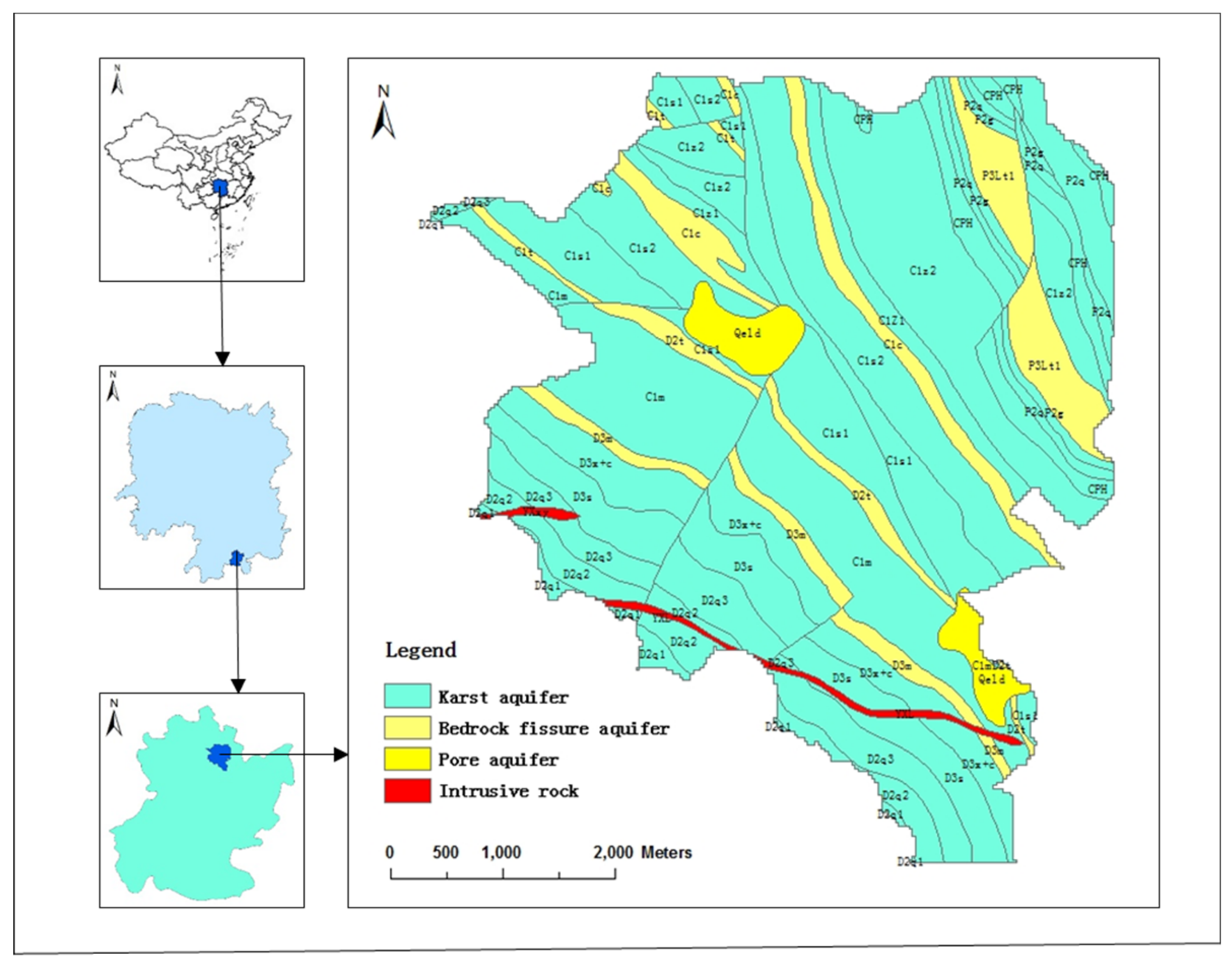
The study area in this paper is located in the Xianghualing area, the north of Linwu County, Hunan province of China (Figure 2). The annual precipitation is 1022.3–1917.4 mm, mostly concentrated in summer. In this region, Devonian and Carboniferous limestone with strong heterogeneousness are the main carriers and media for groundwater. On the surface, circular karst depressions are developed, with funnels and holes on their beneath, and there are caves and rivers underground. In this area, precipitation is the main recharge to the karst aquifer. Surface watershed and insulation boundary constitute the boundary conditions of the study area, and the discharge is located in the northwestern part. The terrain on the south side is higher than that on the north, and conduit flow is the main runoff channels. The tendency direction of the stratum is to the northeast, and the direction of groundwater flow and conduit development are both to the northwest.
3.2. The Improved SWAT Model Established
3.2.1. Data Processed
(1) DEM Processed
DEM (Digital Elevation Model) is a GIS data, describing the spatial distribution of regional geomorphology. The data we used were from the Global Digital Elevation Model with 30 m resolution ratio (GDEM 30M) database downloaded from Geospatial Data Cloud (http://www.gscloud.cn/). The data set is provided by Geospatial Data Cloud site, Computer Network Information Center, Chinese Academy of Sciences. GIS hydrological toolbox and spatial data management toolbox were used to deal with DEM data, such as data splicing, data cutting, filling depression, extracting river network, mask processing and so on. Then we got the DEM diagram containing the terrain factors. Moreover, depressions should be filled in order to reduce river disruption due to data error. In this way, rivers would be generated without disruptions and conform to actual river systems.
(2) Land Use Type Processed
Land use type has an important effect on simulation results and influences the runoff process on the land surface. We cut land use data from Land Cover Products 1.0 of China, with 250 m resolution ratio [23]. The data set is provided by Environmental and Ecological Science Data Center for West China (WESTDC) (http://westdc.westgis.ac.cn). Then we reclassified it and got three land use types, which are “ORCD”, “WATR”, “UINS”, as shown in Figure 3.” ORCD” represents that the land cover type is garden, “WATR” represents that the land cover type is waters and “UINS” represents that the land cover type is public land.
(3) Soil Type Processed and Database
Soil type plays an important role in hydrological cycle in HRUs. Soil data were obtained from the China Soil Map Based Harmonized World Soil Database version 1.1 (HWSD), established by the United Nations Food and Agriculture Organization (FAO) and the international institute for applied systems (IIASA) in Vienna, which provides physical and chemical properties for each grid point [24]. The data set is provided by Cold and Arid Regions Sciences Data Center at Lanzhou (http://westdc.westgis.ac.cn). We clipped the study area from the HWSD data set with 1000 m resolution ratio and reclassified soil type according to the soil physical parameters. If the soil names are the same but their physical parameters are different, it is necessary to define the soils into different types. If the soil names and physical parameters are both consistent, they can be defined as the same type. Finally, the study area is divided into five soil types, as shown in Figure 4.
The physical properties of soil determine the movement of water and gas in the soil profile. It is the key data for the pre-modeling process of SWAT. The values of variables needed for soil database were acquired in three ways: (1) to find the corresponding soil properties from HWSD database; (2) calculated using formula; and (3) calculated by the SWC (Soil Water Characteristics) modules of SPAW software [25,26]. Finally, the three parts of soil attribute data were filled in usersoil format and imported to SWAT2012. mdb.
(4) Meteorological Database
The importance of meteorological data to the hydrological process is obvious. It has a large impact on the entire hydrological cycle system. The meteorological data used in this paper was from China Meteorological Assimilation Driving Datasets for the SWAT model Version 1.0 (CMADS V1.1) [27]. The data set is provided by Cold and Arid Regions Sciences Data Center at Lanzhou (http://westdc.westgis.ac.cn). The CMADS V1.1 data set has been formatted and modified in accordance with the input driver data format of SWAT model, enabling the SWAT model to use the data set directly without any format conversion [28]. There is no meteorological station located inside the study area since the area is small. Therefore, we used the data of four meteorological stations located outside the area but nearest to the study area to calculate the average value of climatic variables as the values of the study area. The data include daily values of precipitation, maximum and minimum temperature, wind speed, relative humidity and solar radiation. The locations of meteorological stations are shown in Figure 5.
3.2.2. The Model Established
In the process of setting up the improved SWAT model, the processed DEM data was used to generate rivers and calculate the direction of flow. In order to lighten computational burden, the watershed range was used as the model mask. In this way, the boundary was defined simultaneously. The river network was divided according to the threshold value of the minimum area in the study catchment. In this paper, the threshold value was set to be 60 ha. Then the whole area was divided into 15 sub-catchments (Figure 6), with a total area of 26.76 km2. The parameter characteristics of each sub-basin have been listed in Table 1. The processed soil map and land use map are necessary to establish SWAT and the corresponding index tables need to be imported in the specified format. For slope classification, SWAT has two standards, i.e., Single Slope and the Multiple Slope. In this paper, we used the Multiple Slope method to divide the basin slope into two levels. Through the combination of land use type, soil type and multiple slopes, the final configuration resulted in 85 HRUs (Hydrological Response Units). The result is demonstrated in Figure 7.
4. Results and Discussion
4.1. Parameter Sensitivity
In this paper, SUFI-2 (Sequential Uncertainty Fitting Version 2) algorithm of SWAT-CUP (SWAT Calibration and Uncertainty Procedures) software was used to analyze the parameter sensitivity of the improved SWAT model. The greater the absolute value of t and the smaller the value of p, the more sensitive the parameter is [29]. According to watershed hydrological processes and the experience, we select three original SWAT parameters and four newly added parameters for global sensitivity analysis. The parameter sensitivity sequence, value ranges and the final values are shown in Table 2. Results show that the newly added parameters are much more sensitive than the original parameters. represents the infiltration proportion from the epikarst reservoir into the quick flow reservoir and it reflects the development degree of the karst fracture, relating to the geological setting and hydraulics of the karst. is the attenuation constant for the up quick flow reservoir and it represents the relative change rate of quick flow. represents the infiltration proportion from the upper quick flow reservoir to lower slow flow reservoir and reflects the development degree of the karst conduit, relating to the geological setting and hydraulics of the karst. is the attenuation constant for the lower slow flow reservoir system and it denotes the relative change rate of slow flow. CN2 is the runoff curve number of SCS (soil conservation service) and it is related to soil type, land use type and slope. RCHRG_DP is the percolation fraction of the deep aquifer and describes the characteristics of the deep aquifer. CH_N2 is Manning’s “n” value for the main channel and describes the characteristic of the main channel.
4.2. Model Evaluation
The daily runoff data observed in the watershed outlet were used to calibrate and validate the model. The simulated results obtained by the improved and original models are in comparison with observed values, as shown in Figure 8. Data from 1 January 2016 to 30 June 2016 were used to calibrate the model parameters. The results show that for the original model, the value of R2 is 0.62 and ENS is 0.63, while the value of R2 is 0.84 and ENS is 0.83 simulated by the improved model. Both the linear correlation and model reliability have been efficiently strengthened with the improvements we proposed. Furthermore, data from 1 July 2016 to 31 October 2016 were used to validate the model. The validation results show that the values of R2 and ENS are 0.82 and 0.81 obtained by the improved model, while for original model, the value of R2 and ENS are merely 0.57 and 0.58. It can be concluded that the improved model outperforms the original one in terms of both the model fitting effect and model quality.
4.3. Discussion
In the karst area of South China, the existence of underground rivers and conduits means that groundwater flow contributes more to the outlet than that of surface flow. So, the parameters involving the groundwater module are much more sensitivity than those of others. The upper quick flow reservoir is an important regulation structure for karst areas. The parameters and describe the characteristics of an upper quick flow reservoir including underground rivers, conduits, big fracture and so on. Due to various characteristics they represent, these parameters are the most sensitive and it is necessary to conduct parameter sensitivity analysis. The parameters and describe the characteristics of lower slow flow reservoir which represents small fissure, and its function is secondarily important to upper quick flow reservoir. Similarly, and are also sensitive parameters relating to a karst area. CN2 is related to the surface characteristics, and RCHRG_DP denotes the water lost from the system. CH_N2 is the parameter concerning the characteristics of the main channel. Consequently, the three parameters above are also sensitive, but less than parameters , , and .
Ens is the efficiency coefficient and R2 is the correlation coefficient. They can indicate the fitting degree between the simulated value and measured value in the simulation process. The range of their values is between 0 and 1. The correlation gets better as their values approach 1. If the value of Ens is greater than 0.5, the simulation value can be regarded within the acceptable range. R2 further reflects the coincidence degree between simulated values and measured values. If R2 = 1, it implies that the coincidence is very good. Otherwise, the lower R2 means the coincidence is not obvious. So, these two parameters are adequate to illustrate the performance of models.
The degree of karstification is very high, and underground rivers are developed in the karst area of South China. It is difficult to acquire much more measured data. We used one year’s meteorological data, including daily values of precipitation, maximum and minimum temperature, wind speed, relative humidity and solar radiation and one year’s measured runoff data. Although the data period is not long enough, they are daily scale data. Compared with existing research from academia, our daily data is more detailed since the other studies’ measured runoff data are just monthly scale. Moreover, results show that our study outperforms on accuracy and reliability. For example, Yang L Y et al. have used the simplified SWAT model to simulate the loading of non-point source pollution in the demonstration area. The data period they use is also one year and their data are in the form of monthly scale [30]. Wei C H et al. have used the SWAT model to simulate a runoff process in Chishui River karst area. Although their meteorological data are in daily scale, their runoff data are just in monthly scale [31]. Liu H et al. have used a SWAT model to evaluate groundwater resources in Lianjiang Basin karst region, and they also used monthly flow rate to determine and verify model parameters [32]. In this paper, we used daily scale data to calibrate and validate the improved SWAT model and original SWAT model. The results show that indicators of ENS and R2 in the improved SWAT model are much larger than that of the original SWAT model both in the calibration and validation period. It is illustrated that the improved model has better simulation performance and can provide a more suitable way for solving the hydrological cycle in the karst areas of South China.
5. Conclusions
In this paper, we conceptualize a karst aquifer system in a three series–parallel linear reservoirs model including epikarst reservoir to describe the characteristic of the epikarst system, quick flow reservoir to describe the recharge–storage–discharge process in the conduit system, and slow flow reservoir to describe the process of recharge–storage–discharge in the micro-fissure system. The three reservoirs model is correlative and represents a complete underground water system. Then we coupled the reservoirs model with the SWAT model to improve the performance of the original SWAT model, making it applicable and effective for simulating hydrological process in karst areas located in southern China.
A small, relatively independent watershed located in Xianghualing region is taken as the study area. The improved SWAT model is applied to simulate the hydrological process in this area. The daily observed data of basin outlet flow in 2016 were used to calibrate and validate the model. Simulation results obtained by the improved model fit well with observed values, which illustrates that the improved model is applicable for hydrological cycle process simulation in the karst area of south China. Compared with the original model, the improved model outperforms in both calibration and validation period, with significant improvements in terms of R2 and ENS. Therefore, the improved SWAT model is verified to have better simulation precision and higher model quality and feasibility than that of the original SWAT model.
Author Contributions
Data curation, Y.C.; formal analysis, Q.Z.; investigation, C.S.; methodology, J.S.; writing—original draft, Y.W.
Funding
This research was funded by (National Key R&D Program of China) grant number (2017YFC0406106).
Conflicts of Interest
The authors declare no conflict of interest.
References
- Jiang, G.H.; Chen, K.K.; Yu, S.; Peng, W. Separating Karst Slope Runoff in Peak Cluster Area. J. China Hydrol. 2009, 29, 14–19. (In Chinese) [Google Scholar]
- Luo, M.M. The Physical Machanism and Methematical Model of Karst Water Circulation: A Case Study of the Xiangxi River Karst Basin, South China; China University of Geosciences: Wuhan, China, 2017. (In Chinese) [Google Scholar]
- Brkić, Ž.; Kuhta, M.; Hunjak, T. Groundwater flow mechanism in the well-developed Karst aquifer system in the western Croatia: Insights from spring discharge and water isotopes. Catena 2018, 161, 14–26. [Google Scholar]
- Kong-A-Siou, L.; Fleury, P.; Johannet, A.; Estupina, V.B.; Pistre, S.; Dörfliger, N. Performance and complementarity of two systemic models (reservoir and neural networks) used to simulate spring discharge and piezometry for a Karst aquifer. J. Hydrol. 2014, 519, 3178–3192. [Google Scholar]
- Kourgialas, N.N.; Karatzas, G.P.; Nikolaidis, N.P. An integrated framework for the hydrologic simulation of a complex geomorphological river basin. J. Hydrol. 2010, 381, 308–321. [Google Scholar] [CrossRef]
- Tzoraki, O.; Nikolaidis, N.P. A generalized framework for modeling the hydrologic and biogeochemical response of a Mediterranean temporary river basin. J. Hydrol. 2007, 346, 112–121. [Google Scholar] [CrossRef]
- Nikolaidis, N.P.; Bouraoui, F.; Bidoglio, G. Hydrologic and geochemical modeling of a karstic Mediterranean watershed. J. Hydrol. 2013, 477, 129–138. [Google Scholar] [CrossRef]
- Zhou, Q.; Chen, L.; Singh, V.P.; Zhou, J.; Chen, X.; Xiong, L. Rainfall-runoff simulation in karst dominated areas based on a coupled conceptual hydrological model. J. Hydrol. 2019, 573, 524–533. [Google Scholar] [CrossRef]
- Zhao, Y.M.; Liao, W.H.; Lei, X.H. Hydrological Simulation for Karst Mountain Areas: A Case Study of Central Guizhou Province. Water 2019, 11, 991. [Google Scholar] [CrossRef]
- Epting, J.; Page, R.M.; Auckenthaler, A.; Huggenberger, P. Process-based monitoring and modeling of Karst springs—Linking intrinsic to specific vulnerability. Sci. Total Environ. 2017, 625, 403–415. [Google Scholar] [CrossRef]
- Ren, Q.W. Water Quantity Evaluation Methodology Based on Modified SWAT Hydrological Modeling in Southwest Karst Area; China University of Geosciences: Wuhan, China, 2006. (In Chinese) [Google Scholar]
- Baffaut, C.; Benson, V.W. Modeling flow and pollutant transport in a Karst watershed with SWAT. Trans. ASABE 2009, 52, 469–479. [Google Scholar] [CrossRef]
- Malagò, A.; Efstathiou, D.; Bouraoui, F.; Nikolaidis, N.P.; Franchini, M.; Bidoglio, G.; Kritsotakis, M. Regional scale hydrologic modeling of a Karst-dominant geomorphology: The case study of the Island of Crete. J. Hydrol. 2016, 540, 64–81. [Google Scholar]
- Wang, Y.; Brubaker, K. Implementing a nonlinear groundwater module in the soil and water assessment tool (SWAT). Hydrol. Process. 2014, 28, 3388–3403. [Google Scholar] [CrossRef]
- Wittenberg, H.; Sivapalan, M. Watershed groundwater balance estimation using streamflow recession analysis and baseflow separation. J. Hydrol. 1999, 219, 20–33. [Google Scholar] [CrossRef]
- Eris, E. Estimation of baseflow and water transfer in Karst catchments in Mediterranean Turkey by nonlinear recession analysis. J. Hydrol. 2015, 530, 500–507. [Google Scholar] [CrossRef]
- Biswal, B.; Marani, M. ‘Universal’ recession curves and their geomorphological interpretation. Adv. Water Resour. 2014, 65, 34–42. [Google Scholar] [CrossRef]
- Wittenberg, H. Baseflow recession and recharge as nonlinear storage processes. Hydrol. Process. 1999, 13, 715–726. [Google Scholar] [CrossRef]
- Ebrahim, G.Y.; Villholth, K.G. Estimating shallow groundwater availability in small catchments using streamflow recession and instream flow requirements of rivers in South Africa. J. Hydrol. 2016, 541, 754–765. [Google Scholar] [CrossRef] [Green Version]
- Griffiths, G.A.; Clausen, B. Streamflow recession in basins with multiple water storages. J. Hydrol. 1997, 190, 60–74. [Google Scholar] [CrossRef]
- Wittenberg, H. Nonlinear analysis of flow recession curves. In FRIEND—Flow Regimes from International Experimental and Network Data; IAHS Publication: Washington, DC, USA, 1994; Volume 221, pp. 61–67. [Google Scholar]
- Chen, S. Quantitative Evaluation Method of Groundwater Resources in Karst Peak Forest Area in Southwest China; China University of Geosciences: Beijing, China, 2018. (In Chinese) [Google Scholar]
- Ran, Y.; Li, X.; Lu, L. Land Cover Products of China. Cold Arid Reg. Sci. Data Cent. Lanzhou 2010. [Google Scholar] [CrossRef]
- Fischer, G.; Nachtergaele, F.; Prieler, S.; van Velthuizen, H.T.; Verelst, L.; Wiberg, D. Global Agro-Ecological Zones Assessment for Agriculture (GAEZ 2008); IIASA: Laxenburg, Austria; FAO: Rome, Italy, 2008. [Google Scholar]
- Saxton, K.E.; Willey, P.H.; Rawls, W.J. Field and Pond Hydrologic Analyses with the SPAW Model. In Proceedings of the 2006 ASAE Annual Meeting. American Society of Agricultural and Biological Engineers, Portland, OR, USA, 9–12 July 2006. [Google Scholar]
- Saxton, K.; Willey, P. The SPAW Model for Agricultural Field and Pond Hydrologic Simulation. In Watershed Models; CRC Press: Boca Raton, FL, USA, 2006. [Google Scholar]
- Meng, X.Y. China Meteorological Assimilation Driving Datasets for the SWAT model Version 1.1. Cold Arid Reg. Sci. Data Cent. Lanzhou 2016. [Google Scholar] [CrossRef]
- Meng, X.Y.; YU, D.L.; Liu, Z.H. Energy Balance-Based SWAT Model to Simulate the Mountain Snowmelt and Runoff—Taking the Application in Juntanghu Watershed (China) as an Example. J. Mt. Sci. 2015, 12, 368–381. [Google Scholar] [CrossRef]
- Abbaspour, K.C. SWAT Calibration and Uncertainty Program—A User Manual; SWAT-CUP-2012; Swiss Federal Institute of Aquatic Science and Technology: Dübendorf, Switzerland, 2012. [Google Scholar]
- Yang, L.Y.; Xia, Y.; Cai, X.F. Applicability evaluation of simulating small watershed of tributary in Lijiang River by simplified SWAT model. J. Water Resour. Water Eng. 2015, 26, 101–104. [Google Scholar]
- Wei, C.H.; He, Z.F.; Zhu, H.B. Runoff Simulation for Karst Area Based on SWAT Model—Taking Chishui River Basin Upstream as An Example. J. Mianyang Norm. Univ. 2015, 34, 98–102. [Google Scholar]
- Liu, H.; Tang, Z.H. Study on Groundwater Resources in Karst Region in SWAT Model. J. Anhui Agri. Sci. 2013, 41, 4559–4561. [Google Scholar]
Figure 1.
Reservoir model structure schematic diagram in the karst area of south China. represents the infiltration water through the epikarst reservoir; represents the injection volume from depression and aven; represents the infiltration proportion from the epikarst reservoir into the quick flow reservoir; represents the infiltration proportion from the quick flow reservoir to slower flow reservoir; represents surface runoff; represents the discharge of quick flow reservoir; represents the discharge of slower flow reservoir.

Figure 2.
Location of the study area.

Figure 3.
Classification of land use type.

Figure 4.
Classification of soil type.

Figure 5.
The locations of flow monitored and meteorological stations.

Figure 6.
The division of sub basin.

Figure 7.
The division of Hydrological Response Units (HRUs).

Figure 8.
The simulated values before and after model improvement fitting with measured values.


Table 1.
Parameter characteristic values of sub-basins.
| Subbasin | Area (ha) | % | Elev (m) | Subbasin | Area (ha) | % | Elev (m) |
|---|---|---|---|---|---|---|---|
| 1 | 395.64 | 14.78 | 565.09 | 9 | 90.72 | 3.39 | 632.42 |
| 2 | 139.95 | 5.23 | 643.34 | 10 | 454.23 | 16.97 | 620.16 |
| 3 | 196.38 | 7.34 | 705.95 | 11 | 130.95 | 4.89 | 698.28 |
| 4 | 266.67 | 9.97 | 699.38 | 12 | 76.14 | 2.84 | 694.63 |
| 5 | 66.42 | 2.48 | 735.20 | 13 | 115.29 | 4.31 | 626.43 |
| 6 | 60.30 | 2.25 | 717.04 | 14 | 92.07 | 3.44 | 667.73 |
| 7 | 209.61 | 7.83 | 633.32 | 15 | 258.66 | 9.673 | 660.26 |
| 8 | 123.03 | 4.60 | 627.05 |
Table 2.
The value ranges and final value of important parameters.
| Parameter | Value Range | Final Value |
|---|---|---|
| 0.50–1.00 | 0.73 | |
| 0.05–0.20 | 0.09 | |
| 0.10–0.50 | 0.35 | |
| 0.02–0.06 | 0.04 | |
| CN2 | 35–98 | 74 |
| RCHRG_DP | 0.10–1.00 | 0.33 |
| CH_N2 | 0.01–0.30 | 0.20 |
© 2019 by the authors. Licensee MDPI, Basel, Switzerland. This article is an open access article distributed under the terms and conditions of the Creative Commons Attribution (CC BY) license (http://creativecommons.org/licenses/by/4.0/).
Share and Cite
MDPI and ACS Style
Wang, Y.; Shao, J.; Su, C.; Cui, Y.; Zhang, Q. The Application of Improved SWAT Model to Hydrological Cycle Study in Karst Area of South China. Sustainability 2019, 11, 5024. https://doi.org/10.3390/su11185024
AMA Style
Wang Y, Shao J, Su C, Cui Y, Zhang Q. The Application of Improved SWAT Model to Hydrological Cycle Study in Karst Area of South China. Sustainability. 2019; 11(18):5024. https://doi.org/10.3390/su11185024
Chicago/Turabian StyleWang, Yufeng, Jingli Shao, Chuntian Su, Yali Cui, and Qiulan Zhang. 2019. "The Application of Improved SWAT Model to Hydrological Cycle Study in Karst Area of South China" Sustainability 11, no. 18: 5024. https://doi.org/10.3390/su11185024
Note that from the first issue of 2016, this journal uses article numbers instead of page numbers. See further details here.