Impacts of Land-Use Change on Habitat Quality during 1985–2015 in the Taihu Lake Basin

Abstract

Habitat quality (HQ) is of great significance to regional sustainable development, which is a key link for regional ecological security and human welfare. Assessing the temporal and spatial evolution of HQ caused by land-use change could provide a scientific basis for regional ecological protection and land management. Here, based on the ArcGIS platform and the InVEST model, this study quantified the spatial and temporal evolutions of land use, landscape patterns, and HQ from 1985 to 2015, in Taihu Lake Basin (TLB). Hotspot analysis tools were used to identify the spatial agglomeration and evolution characteristics of HQ in TLB. The results showed that, (1) the land use and landscape pattern in TLB experienced dramatic change process during 1985–2015, with the dominating conversion being from farmland to construction land, which led to an increase in landscape heterogeneity and fragmentation. (2) The HQ was generally reduced in the past 30 years. In particular, the decline of HQ was extremely severe in the peripheral area of cities and roads, due to urban sprawl. (3) Regarding the spatial distribution of HQ, the northern and eastern areas were generally higher, while the western and southern areas were generally lower. The hotspots areas were mainly located in the southwestern mountain area and west-central lake area, while the cold spots areas were mainly located in urban areas in the north and the east. (4) The area and degree of habitat degradation were both increased significantly due to land-use change, and the degradation of the Taihu Lake was highlighted. Strengthening the ecological environment management and reducing the threat of urban expansion to the HQ is urgently required. This study could help understand HQ of the TLB and provide a scientific basis for decision-makers.

1. Introduction

Biodiversity refers to variability among organisms from all ecosystems, including terrestrial, marine, and other aquatic ecosystems, and the ecological complexes to which they belong [1]. As one of the most important indicators of ecosystem health assessment [2], the significance of biodiversity to human welfare, human survival, and the global economy are increasingly valued and widely accepted [3]. To meet human needs, human activities directly affect land use and change landscape pattern [4], specifically, extensive urbanization and industrialization require large amounts of land, leading to dramatic changes in land use and landscape patterns [5], causing land fragmentation and reducing the connectivity of habitat patches [6]. Thus, affecting the material and energy flow of the ecosystem, and ultimately causing environmental problems [7], resulting in biodiversity decline, natural habitat destruction, and loss of ecosystem services (ES) [8,9]. Biodiversity resources can not only be directly used as food, medicine, energy, and industrial raw materials, but also indirectly provide ES, including regulating climate, maintaining the stability of natural ecosystems, degrading waste, maintaining natural gene banks, and aesthetic values [10]. The loss of biodiversity due to the increase in the intensity of human activities has received widespread attention from the international community [3,11]. Studies have shown that habitat quality (HQ) can characterize regional biodiversity levels to some extent [12]. HQ refers to the ability of ecosystems to provide appropriate conditions for the persistence of individuals and populations [13], which often depends on the intensity of human activities [14].

Human activities have a profound impact on the environmental quality [15], and land use—the most direct manifestation of human activities—is an important factor threatening HQ [16,17]. Land-use change alter the structure and composition of regional habitats, and then affect the material flow and energy flow cycle between habitat patches, thus changing the regional habitats, production capacity, and service functions [13,18,19]. Previous studies have found that HQ decrease with the increase of adjacent artificial land use [20,21]. Changes in HQ caused by land-use change have become an important reference for ecological environmental protection and land use management [4,22].

Scholars have explored many ways to strengthen the study of HQ [23,24], including the construction of evaluation index systems and the development of model evaluation. Index system method generally focuses on the assessment of habitat suitability, which might require prior information on species distribution or presence [11], and tends to ignore the impact of threat sources [25]. Model evaluation can quantify the HQ and map it, and even predict the future trend of HQ change under different development situations, by combining land-use change simulation models [26]. It has been absorbed and applied by more and more researchers. In recent years, people have gradually realized the impact of threat sources on HQ and gradually incorporated them into study models [27]. The model evaluation method can evaluate the HQ by the distribution of habitats, threat sources, and their interaction condition.

The Integrated Valuation of Environmental Services and Tradeoffs (InVEST) model was jointly developed by Stanford University, the University of Minnesota, the Nature Conservancy, and the World Wildlife Fund [11]. It is one of the most widely used software for evaluation and spatialization of ES [28], with the most detailed routine for evaluation of biodiversity [15]. It has been extensively used in ES assessments around the world and has proven to be robust [29,30,31]. There are two different perspectives to approaching the relationship between biodiversity and ES—the ES perspective and the conservation perspective; the former think hold that biodiversity and ES are equivalent, while the latter believes that biodiversity is a type of ES [1]. Biodiversity has its own intrinsic value within natural systems, thus the biodiversity module on InVEST should be considered to be an independent attribute rather than an ES [28]. The InVEST HQ module can provide rapid assessment for the impacts of different threats and land-use types on biodiversity. The HQ module is promising for estimating HQ that combines information on land use and land cover change (LUCC), accessibility to sources of threats, threats to biodiversity, the sensitivity of habitat to threats, and a half-saturation constant to generate HQ maps [12]. Detailed information on the model, working principles, data needs, results interpretations, as well as model limitation can be found in the InVEST 3.7.0 user’s guide [12]. The model has the advantages of fewer parameters, easy access to parameters, simple operation, and simple data processing [32]. Therefore, it has been widely used in HQ assessment around the world [11,33,34,35], which have been proven to be helpful for the resources and environment management and land-use planning [36]. However, the current research mostly focuses on nature reserves and single species habitats [37], and pays insufficient attention to the changes in HQ in large cities and large watersheds.

Urbanization is an unavoidable global process—since the reform and opening-up policy, China has experienced a rapid urbanization and industrialization process. Problems of a deteriorating ecological environment has accompanied the rapid social and economic development, and this has now been receiving increasing attention [38,39]. Being one of the most developed areas in China, the Taihu Lake Basin (TLB) has been affected by dramatic land-use change in the past decades. TLB is an important ecological function protection area, the ecosystem health of TLB is of great significance for maintaining the ecological balance and sustainable development of the TLB and the development of the Yangtze River Delta integration. Under the interference of high-intensity human activities and large-scale urbanization, the land-use patterns and ES functions have changed significantly [40], which has caused a remarkable change in landscape and environmental deterioration [41,42]. The HQ in this area has faced enormous human disturbance threats, therefore, it is urgent to maintain the HQ and protect the biodiversity in this basin.

In recent years, the ES such as purified water source [43], carbon fixation and oxygen release [44], water quality regulation [45], and crop yield [46] in TLB have been significantly degraded. Degradation of ES have seriously affected human life and health, harmed human well-being, and might further restrict local socio-economic development, threaten regional ecological security, hinder regional sustainable development. Previous studies have been conducted on the ES in the TLB [40,41,47,48], or the habitat environment quality in some parts of the TLB [6,49]. However, there is a lack of individual and specific study on the HQ of TLB, especially the long-term biodiversity research in the TLB still appears to be insufficient. Research on impacts and threats of land-use change on biodiversity, under the interference of anthropogenic activities, need to be strengthened.

Human activities often cause a dramatic reduction of biodiversity, especially in the deltaic areas [50,51], the application of biodiversity research approach in these areas is of great significance [51]. Therefore, it is necessary to conduct a systematic evaluation of the HQ in TLB for decision-making regarding a sustainable development of the basin [52]. Given the importance of the TLB in the sustainable development of the Yangtze River Delta, it is urgent to gain a more comprehensive understanding of the HQ under the land-use change driven by human activities. In this study, we employed the ArcGIS platform and HQ module of the InVEST model for the evaluation of the HQ on the basis of a long time-series (1985–2015) land-use data. Specifically, this study aimed to (1) reveal the temporal and spatial variation of land-use change over the past three decades; (2) evaluate the HQ and habitat degradation pattern and their changes over 30 years, based on the InVEST model; and (3) investigate the hotspots of HQ change in TLB. The results might provide scientific information for governmental departments to enhance sustainability in ecosystem management and land resource utilization, and to positively influence the improvement of HQ in TLB.

2. Materials and Methods

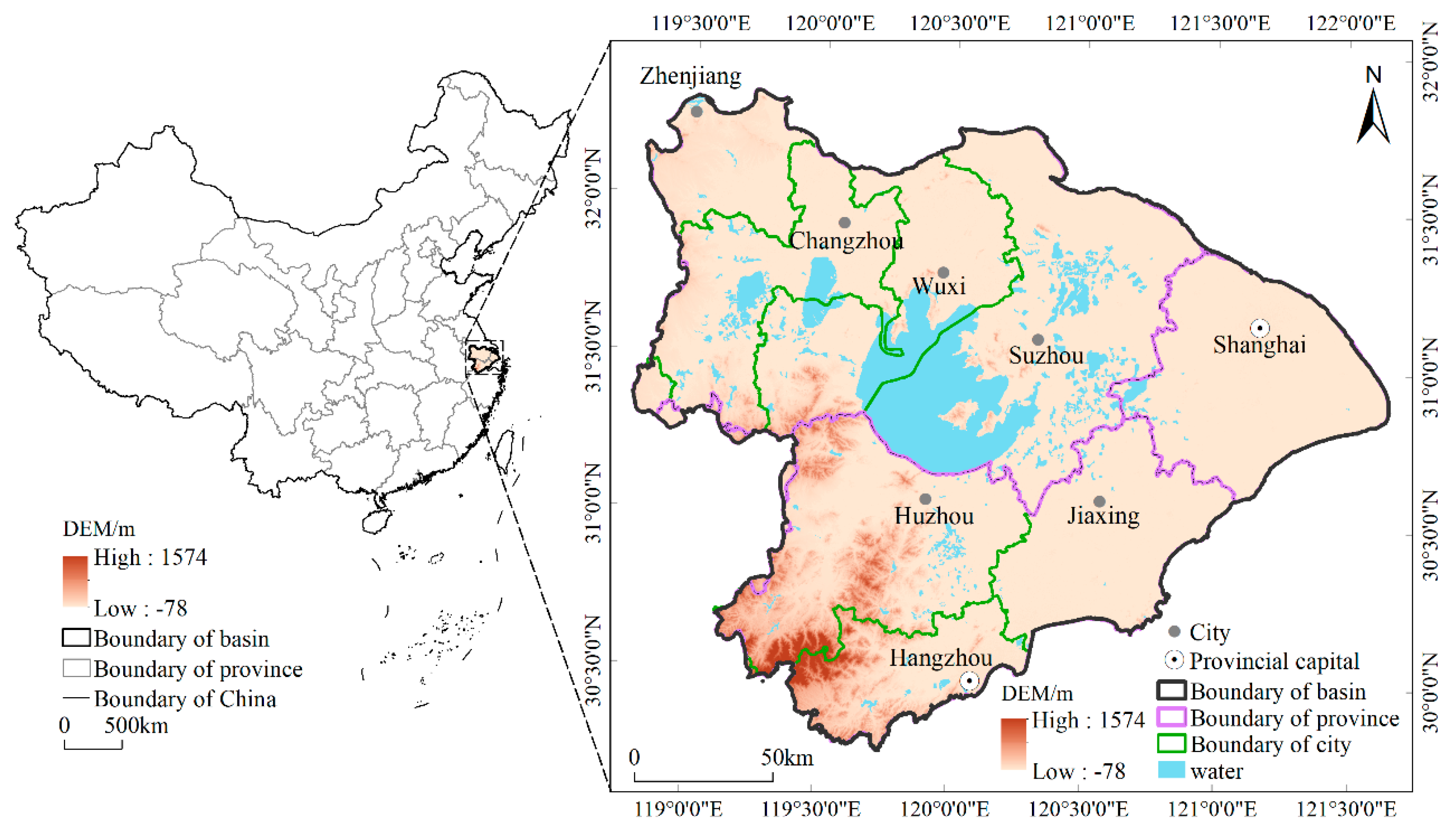
2.1. Study Area

The TLB (30°7′19″–32°14′56″ N, 119°3′1″–121°54′ 26″ E) is the core area of the Yangtze River Delta, which is located in the lower portion of the Yangtze River (Figure 1). It has an area of approximately 36,900 km², with a complex river network and numerous lakes, of which the river density is about 3.4 km/km² [53]. There are more than 200 rivers and 9 lakes with an area over 10 km² in the basin, whereby the Taihu Lake (2427.8 km²) is the largest lake in the basin and the third largest freshwater lake in China [54]. The average elevation of the TLB is 34.4 m, and there are two types of terrains in the TLB—mountains and plains. The TLB is dominated by plains, which are mainly distributed north, east, and south of the basin, accounting for 4/6 of the total area, with water surface accounting for 1/6, while the rest are hilly and mountainous areas, which are mainly distributed southwest of the basin. In the administrative unit, the TLB includes the Shanghai Municipality, the Northern Zhejiang Province, the Southern Jiangsu Province, and a small part of the Western Anhui Province. The TLB is a region with the fastest urbanization, the densest population, the most developed economy, the highest degree of land intensification, and the fastest change in land use.

The population of TLB was nearly 60 million in 2015, with 4.4% of the national population and 0.38% of the national land area, TLB contributed to 9.9% of China’s gross domestic product (GDP) in 2015 (RMB 6,688.4 billion) [55], which has been a great contribution to the socioeconomic development of China [56]. TLB has always been the pioneer zone of urbanization in China, it has been, without a doubt, the most prosperous and dynamic region in the economic development in China [57], meanwhile, it is also one of the most prominent sites of competition between the supply of ES and human demand in China [41]. With the rapid development of urbanization and industrialization, the ecological and environmental problems in the TLB are facing tremendous pressure. The contradiction between human activities and land protection has caused enormous pressure on the ecological carrying capacity and sustainable development capacity of the basin [48].

2.2. Data Collection

The Land use and land cover (LULC) vector data in 1985, 1995, and 2005 were obtained from the National Earth System Science Data Sharing Infrastructure, National Science and Technology Infrastructure of China (http://www.geodata). LULC data in 2015 was provided by the Data Center for Resources and Environmental Sciences, Chinese Academy of Sciences (RESDC) (http://www.resdc.cn/) [58]. Their spatial resolutions were both 30 m, and they used the same classification system of land-use types, which was the Chinese Academy of Sciences classification system of land-use monitoring using remote sensing [59,60]. According to the land resources and their utilization attributes, the TLB area was divided into six first-level land-use types—farmland, forestland, grassland, water, construction land, and unutilized land. According to the natural attributes of land resources, second-level land-use types can be classified on the basis of first-level land-use types. Consequently, farmland was divided into paddy field and dry land; forestland was divided into forest land, shrubland, open forest land, and other woodland; grassland was divided into high coverage grassland, medium coverage grassland, and low coverage grassland; water was divided into river canal, lake, reservoir, and pond, shallows, and bottomland; construction land was divided into urban land, rural land, and industrial and mining land.

DEM (Digital Elevation Model) data with a 30 m spatial resolution, used for the division of the basin, was also obtained from the Resources and Environmental Science Data Center of the Chinese Academy of Sciences (http://www.resdc.cn). The vector data of the latest roads, including main roads (national roads and provincial roads), minor roads (county roads and rural roads), and railways were obtained from the National Basic Geographic Information System (http://nfgis.nsdi.gov.cn) of China. Then, according to the latest roads data and the maps of China’s tourism traffic of 1985, 1995, 2005, and 2015, vectorization correction was carried out year by year, and the roads data of each year was finally obtained. The protected area layers were set up with reference to relevant research [61], among which, the basic farmland ecological protection layer and banned construction layer were vectorized using the ArcGIS software, according to the text and related maps of Land Use Master Plan published on the website of each city’s Land and Resources Bureau (2006–2020). The water restricted areas were lakes with an area of more than 10 km² in the study area, and other areas were non-protected areas.

Based on the comprehensive analysis of the size of the study area and the efficiency of the model calculation, and by reference to relevant research literature [26,62,63], we found that data with a spatial resolution of 100 m can avoid the existence of fragmented habitats and reserve enough effective information [62]. Moreover, after several tests, it turned out that the modeling efficiency could be improved significantly after the conversion of data resolution. We finally determined to set a 100 m grid as the research scale, the resolution of all raster data layers was resampled as 100 m × 100 m.

2.3. Research Method

2.3.1. Land-Use Change and Landscape Pattern Analysis

Land-use change, including area change in each land-use type and their mutual conversion, was analyzed and visualized through statistics and intersection tools in the ArcGIS 10.2 platform. Landscape pattern was revealed by the Fragstats software (version 4.2). Considering the characteristics of the metrics and by referring to other studies [62,64,65,66,67], the metrics that are commonly used and have been proven to be well-represented were selected to represent the landscape pattern. They are the Largest Patch Index (LPI), Mean Patch Size (MPS), Landscape Division Index (DIVISION), Contag Index (CONTAG), Landscape Shape Index (LSI), and Shannon’s Diversity Index (SHDI). A brief introduction was shown in

Table 1. Descriptions of the landscape-level metrics selected.

Metrics	Name and Ecological Meaning
LPI	Largest Patch Index is the proportion of the largest patches in a landscape type to the whole landscape area; it reflects the dominant species in the landscape.
MPS	Mean of Patch Size represents an average condition; a plaque with a smaller value has more fragments than a plaque with a larger value.
DIVISION	Landscape Division Index reflects the degree of separation of the landscape; the closer the value is to 1, the higher the degree of division of the landscape type.
CONTAG	Contag Index means the degree of agglomeration of the landscape; the larger the value, the higher the degree of plaque agglomeration and better the connectivity.
LSI	Landscape Shape Index indicates the complexity of the shape of the landscape; the larger the value, the more complex the shape.
SHDI	Shannon’s Diversity Index shows the changes of the number and proportion of landscape types. In a landscape system, the richer the land use, the higher the degree of fragmentation, the greater the uncertainty of the information content, and the higher the SHDI value.

and their detailed meaning can be found in the help manual of Fragstats [68].

2.3.2. Habitat Quality Module in InVEST and Its Parameterization

The HQ module in InVEST was used to evaluate and map the HQ in the TLB. The HQ Module is a spatially explicit model that uses HQ as a representative of biodiversity associated with different LULC categories [12]. The hypothesis of the model is that regions with a higher HQ can support higher local species richness, and the decline of habitat range and quality will lead to a decline in species persistence [11]. The HQ is a function of four factors: (1) each threat’s relative impact, (2) the relative sensitivity of each habitat type to each threat, (3) the distance between habitats and sources of threats, (4) and the degree to which the land is legally protected [12]. Habitat degradation needs to be calculated first, as shown in Equation (1):

$$D_{xj}={\displaystyle {\sum }_{r=1}^R{\displaystyle {\sum }_{y=1}^{Y_r}\left(\frac{w_r}{{\displaystyle {\sum }_{r=1}^R{w}_r}}\right)}}{r}_y{i}_{rxy}{\beta }_x{S}_{jr}$$

(1)

where $D_{xj}$ is the habitat degradation or total threat level of LULC type $j$ in a grid cell $x$; $R$ is the number of threat factors; $r$ presents the threat layer; $y$ indicates all grid cells on a raster map of $r$; $Y_r$ indicates the set of grid cells on a raster map of $r$; $w_r$ indicates the weight of each threat factor (value from 0 to 1); $r_y$ indicates the effect of threat $r$ that originates in grid cell $y$; $i_{rxy}$ indicates the distance between habitat and the threat source and the impact of the threat across space; ${\beta }_x$ is the factor that may mitigate the impact of threats on habitat through various protection policies (here, ${\beta }_x$ = 1); and $S_{jr}$ indicates the sensitivity of LULC type $j$ to threat factor $r$, where values closer to 1 indicate greater sensitivity, (if $S_{jr}$ = 0, then $D_{xj}$ is not a function of threat $r$).

A half-saturation function is used to interpret a raster cell degradation score into HQ. The degradation of the grid unit increases its HQ by reducing the HQ of the plaque group in the LULC type $j$. The HQ is represented by $Q_{xj}$, as shown in Equation (2):

$$Q_{xj}=H_j\left(1-\frac{D_{xj}^2}{D_{xj}^2+k^z}\right)$$

(2)

where, $Q_{xj}$ means the HQ of LULC type $j$ in a grid cell $x$; $H_j$ indicate the habitat suitability of LULC type $j$; $k$ is the half-saturation constant; $z$ is normalized constants, $z$= 2.5 is set as programmed. The final HQ values range from 0 to 1, 1 indicating the highest level of HQ and 0 indicating non-habitat.

The modeling results of the final HQ are relative values that range from 0 to 1. Areas with higher values indicate better HQ, 0 indicates a non-habitat LULC type and the lowest level of HQ, while 1 indicates a perfect habitat LULC type and the highest level of HQ. In addition to identifying the status of HQ, the model can also visualize the spatial distribution of HQ and habitat degradation of the study area, by combining the ArcGIS 10.2 software. HQ and habitat degradation in TLB were further divided into five grades by the natural breaks (Jenks) method in the ArcGIS, statistics on the area ratio of HQ at different grades were calculated.

The data requirements for the HQ module in the InVEST include the LULC map, threat factors data, sources of threats, accessibility to sources of degradation, habitat types, and their sensitivity to each threat. With reference to related research [69], threats sources in this study were assigned into the urban land, rural land, industrial and mining land, farmland, unutilized land, and roads. Whereas, farmland, forestland, grassland, and water were considered to be natural habitat types. The accessibility to sources of degradation included a basic farmland ecological protection layer and a banned construction layer. The distance between habitats and sources of threats, weight, decay type of threats factors, and the sensitivity of habitats to threat factors were derived from previous studies [25,70,71], and the InVEST Model user’s guide manual [12], see

Table 2. Threat factors and their maximum distance of influence, weight, and type of decay over space.

Threat Factors	Maximum Distance of Influence/km	Weight	Type of Decay Over Space
Urban land	10	1.00	Exponential
Rural land	5	0.60	Exponential
Industrial and Mining land	6	0.50	Exponential
Paddy field	8	0.70	Linear
Dry land	8	0.60	Linear
Unutilized land	1	0.50	Linear
Railway	5	0.70	Linear
Main roads	3	0.60	Linear
Minor roads	2	0.50	Linear

for details. The sensitivity of land-use type to threats factors is shown in

Table 3. The sensitivity of land-use type to habitat threat factors.

LULC	Habitat Suitability	Urban Land	Rural Land	Industrial and Mining Land	Unutilized Land	Paddy Fields	Dry Land	Railway	Main Roads	Minor Roads
PF	0.60	0.50	0.35	0.20	0.30	0.00	0.10	0.70	0.60	0.50
DL	0.40	0.50	0.35	0.20	0.30	0.20	0.00	0.60	0.55	0.45
FL	1.00	1.00	0.85	0.60	0.50	0.80	0.70	0.70	0.70	0.70
SL	0.95	0.60	0.45	0.40	0.40	0.50	0.40	0.70	0.70	0.70
OFL	0.90	1.00	0.90	0.65	0.55	0.85	0.75	0.75	0.75	0.65
OWL	0.85	1.00	0.95	0.70	0.50	0.90	0.80	0.75	0.75	0.65
HCG	0.80	0.60	0.45	0.40	0.60	0.40	0.40	0.50	0.55	0.60
MCG	0.75	0.65	0.50	0.45	0.60	0.45	0.45	0.55	0.60	0.70
LCG	0.70	0.70	0.55	0.50	0.60	0.50	0.50	0.60	0.65	0.70
RC	1.00	0.85	0.70	0.50	0.40	0.80	0.70	0.50	0.70	0.40
LK	1.00	0.90	0.75	0.55	0.45	0.85	0.75	0.50	0.70	0.40
RP	1.00	0.85	0.75	0.55	0.45	0.85	0.75	0.50	0.70	0.40
SH	0.60	0.95	0.80	0.60	0.50	0.70	0.60	0.50	0.80	0.50
BL	0.60	0.95	0.80	0.60	0.50	0.70	0.60	0.50	0.80	0.50

Note: PF—paddy fields; DL—dry land; FL—forest land; SL—shrubland; OFL—open forest land; OWL—other woodland; HCG—high coverage grassland; MCG—medium coverage grassland; LCG—low coverage grassland; RC—river canal; LK—lake; RP—reservoir and pond; SH—shallows; and BL—bottomland.

.

2.3.3. Hotspots Analysis

Hotspot analysis was used to study the local area clustering distribution characteristics, which can be used to test whether there are statistically significant high and low values in the spatial distribution of HQ. We employed the Getis-Ord G* index to identify statistically significant spatial clusters of high values (hotspots) and low values (cold spots) of HQ in the TLB. This indicator can be used to reveal the agglomeration of HQ in local space. Based on the ArcGIS platform, by looking at each HQ values of a grid within the context of neighboring HQ values, the HQ values of each grid and its neighbors were compared proportionally to the sum of all grids. When the G* value was significantly positive, the HQ showed a high-value concentration, which was a hotspot area. While when the G* value was significantly negative, the HQ was low-value aggregation, which was a cold spot area [72]. This method identified hotspots and cold spots through the significant levels—the area corresponding to the G* value at the 99% significant level was regarded as the hotspots and the cold spots, and the area corresponding to the G* value at the 95% significant level was the sub-hotspots and the sub-cold spots [73]. The calculation formula was:

$$G_i^{*}=\frac{{\displaystyle {\sum }_{j=1}^n{w}_{ij}{x}_j-\overline{x}{\displaystyle {\sum }_{j=1}^n{w}_{ij}}}}{S\sqrt{\frac{{\left[n{\displaystyle {\sum }_{j=1}^n{w}_{ij}^2-\left({\displaystyle {\sum }_{j=1}^n{w}_{ij}}\right)}\right]}^2}{n-1}}}$$

(3)

where, $x_j$ is the HQ of raster $j$; $w_{ij}$ is the spatial weight matrix of raster $i$ and raster $j$, if $i$ and raster $j$ are adjacent, their spatial weight is 1, otherwise 0; $\overline{x}$ is the average HQ value; $S$ is the standard deviation of HQ value; and $n$ is the total raster number.

3. Results

3.1. Land-Use Change in TLB from 1985 to 2015

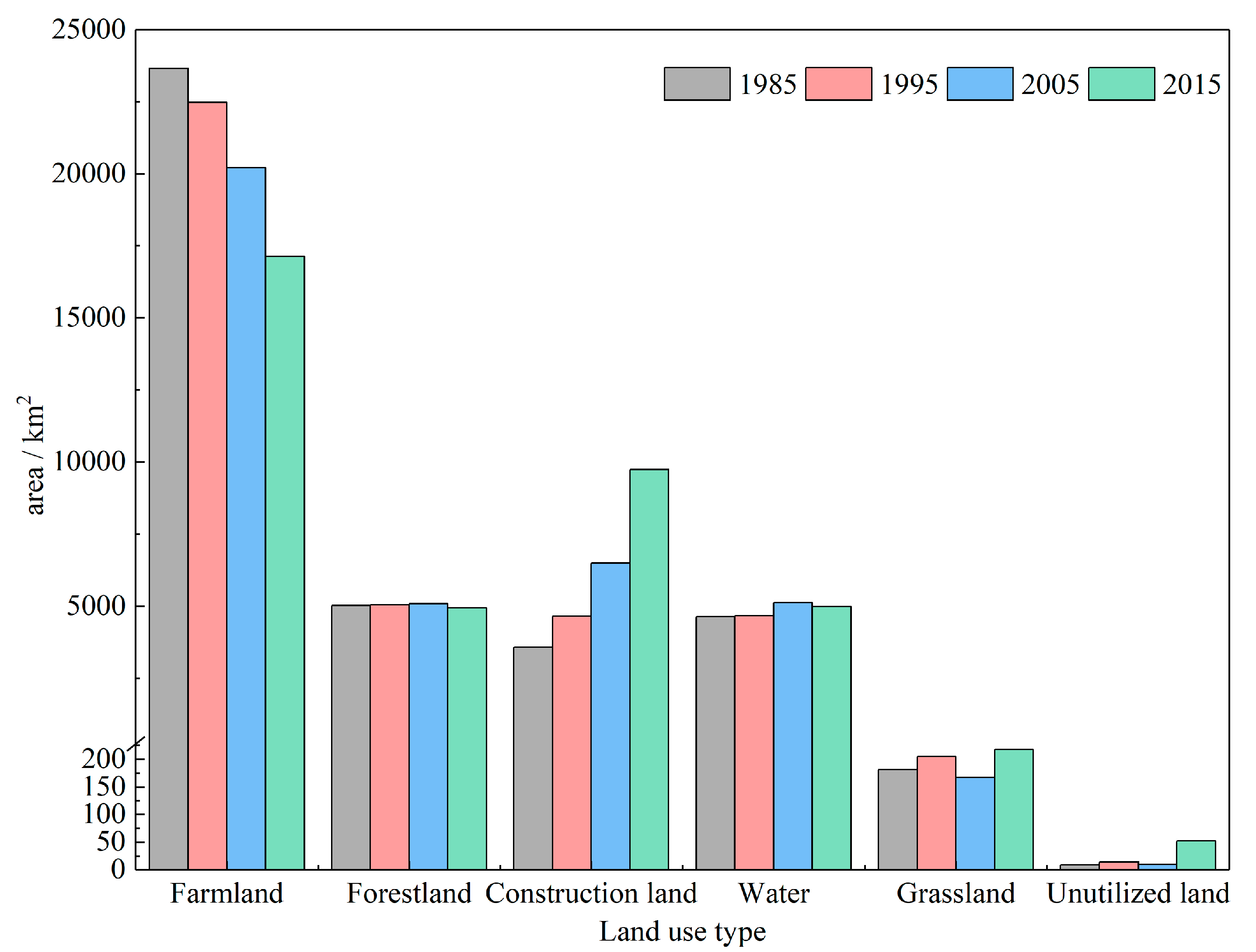
3.1.1. Spatial-Temporal Characteristics of Land-Use Change

The TLB is a place of population agglomeration and economic prosperity with a high degree of land artificialization. The land-use types in the TLB mainly include farmland, forestland, construction land and water, these land-use types constitute the landscape matrix, and the proportions of grassland and unutilized land are much smaller. The spatial distribution of each land-use types has its own characteristics (Figure 2). The TLB has a flat terrain and superior climatic conditions, which is suitable for agricultural cultivation. Farmland is the most widely distributed, forestland is mainly distributed in the southwest mountainous area of the basin, while the construction land is mainly concentrated around cities, especially Shanghai, Suzhou, Wuxi, Changzhou, and Hangzhou. With densely covered rivers and complicated water systems in the watershed, there are lots of rivers and lakes, such as the Taipu River and Taihu Lake.

The area of each land-use type in 1985, 1995, 2005, and 2015 are shown in Figure 3. The TLB has undergone a relatively strong process of land-use change. Specifically, the area of farmland decreased significantly, with a decrease of 6,523.16 km², the forestland reduced slightly, water, grassland, construction land, and unutilized land increased by varying degrees. The construction land expanded dramatically, with an increase of 6,160.39 km², the area of construction land in 2015 was about 2.72 times that of 1985. Water, grassland, and unutilized land increased by 359.49 km², 36.67 km², and 43.46 km², respectively. Obviously, the rapid expansion of construction land and the dramatical reduction of farmland were the main characteristics of land-use change in the TLB during the past 30 years.

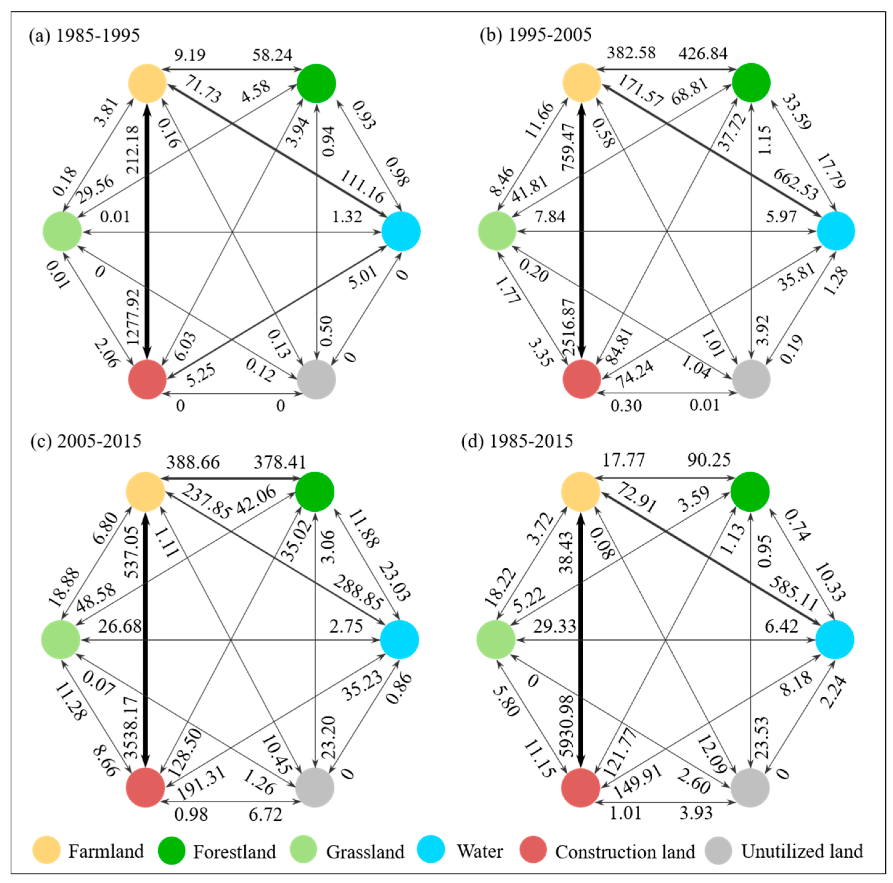
3.1.2. Land-Use Transition Matrix

To further clarify the interaction between each land-use type in the process of rapid urbanization, a land-use transition matrix was constructed and visualized. The land use of the transition matrix was conducted every 10 years (Figure 4).

During the 30 years, land conversion occurred between almost each two land-use types. Among which, the most notable characteristic was a transformation from farmland into construction land. There were 1,277.92 km² (Figure 4a), 2,995.36 km² (Figure 4b), and 3,331.99 km² (Figure 4c) of farmland, which was transformed into construction land, in the three periods, respectively. From the whole research period (Figure 4d), there was a total of 5,390.98 km² of farmland transformed into construction land, whereas the conversion area from construction land into farmland was only 38.43 km². It indicated that urban spatial expansion mainly depended on encroaching farmland during the process of rapid urbanization. In addition, a small amount of farmland was transformed into water or forestland, and was rarely transformed into other land-use types. The main reason for farmland to water transition is that local farmers have spontaneously excavated farmland into ponds for aquaculture, in order to obtain a higher income. The transition area between other land-use types was relatively small. However, it is worth noting that the transition from water to construction land was rather small from 1985 to 1995, but this conversion area increased to 74.24 km² from 1995 to 2005, and 191.31 km² from 2005 to 2015. This indicated that the shrinkage of the water area was increasingly serious under the surge of urbanization and industrialization. For instance, some water was gradually occupied by urban construction and industrial development, due to their advantage of water resources and ecological environment.

3.1.3. Landscape Pattern Index Change

The results of the landscape level analysis are shown in

Table 4. Landscape pattern index at the landscape level of the TLB in 1985, 1995, 2005, and 2015.

Years	LPI	MPS	LSI	CONTAG	DIVISION	SHDI
1985	60.20	116.02	102.09	59.28	0.63	1.07
1995	57.30	124.74	103.89	57.41	0.66	1.13
2005	47.54	144.60	108.92	54.45	0.76	1.21
2015	19.99	131.69	115.74	51.51	0.92	1.29

. From 1985 to 2015, LPI reduced from 60.20 to 19.99, indicating that as the proportion of large area patches decreased, landscape patches become more fragmented. MPS increased from 116.02 to 131.69, which meant that the average area of landscape patches increased slightly. The LSI increased from 102.09 to 115.74, which revealed that the degree of plaque aggregation was reduced and the shape tended to be complex. The CONTAG decreased from 59.28 to 51.51, implying that the degree of patches accumulation in the landscape reduced and the connection among the patches declined. The DIVISION increased from 0.63 to 0.92, indicating that the complexity of the landscape structure increased and the overall fragmentation trend increased. The SHDI increased from 1.07 to 1.29, indicating that in the landscape system, the diversity and heterogeneity in patches increased, as well as the complexity of the landscape structure. Due to the significant expansion in construction land and dramatic farmland losses, other land types changed to a relatively lesser extent, thus the difference in the proportion of the landscape components of each type became smaller, causing an increase in the SHDI. Overall, although the MPS and SHDI in the TLB had increased, the rising LSI and DIVISION and the decreasing CONTAG indicated that the landscape fragmentation in TLB had increased. The landscape level index revealed that landscape pattern was more complicated and the degree of fragmentation of landscape structure has been deepening in the TLB, over the past three decades. This situation resulted in increasing pressure in maintaining ecological balance and biodiversity, and led to the degradation of HQ in TLB.

3.2. Habitat Quality

The HQ results of the TLB in 1985–2015 is shown in

Table 5. Ratio of each HQ level of the TLB in 1985, 1995, 2005, and 2015 (%).

Grades	Value Range	1985	1995	2005	2015
		Ratio/%	Ratio/%	Ratio/%	Ratio/%
Poor	0.00–0.20	9.71	12.60	17.58	26.42
Relatively poor	0.20–0.40	4.95	4.25	3.75	3.34
Moderate	0.40–0.60	56.87	54.50	48.85	41.24
Relatively good	0.60–0.80	2.59	2.61	2.41	2.31
Good	0.80–1.00	25.88	26.04	27.41	26.70
Mean value		0.63	0.62	0.59	0.54

and Figure 5. From the perspective of time variation, in general, the HQ showed a significant downward trend, and the average HQ were 0.63 in 1985, 0.62 in 1995, 0.59 in 2005, and 0.54 in 2015. The area ratio of HQ at different grades is shown in Table 5. During the study period, most of the study area was at the moderate level of HQ. The area of moderate-quality habitats in the study area decreased significantly, from 56.87 % in 1985 to 41.24 % in 2015. While the area of poor-quality habitats increased significantly, from 9.71 % in 1985 to 26.42 % in 2015. The area of other grades changed relative slightly. The average of HQ dropped from a relatively good grade in 1985 (0.63) and 1995 (0.62), to the moderate level in 2005 (0.59) and 2015 (0.54).

From the perspective of spatial distribution, HQ distribution is shown in Figure 5. There was a significant change in spatial distribution variability in the TLB. The minimum HQ value was 0, which appeared in the non-habitat LULC type, i.e., construction land, and the maximum HQ value was 1, which appeared mainly in mountainous areas and water areas. The spatial distribution pattern of HQ was lower in the north and the east than in the south and west, which was similar to the land-use distribution. The northern and eastern parts of the TLB are dense urban areas with a high proportion of construction land. The western and southern regions have a large number of waters and mountains, where cities are relatively less dense than the northern and eastern regions. Forests in the mountainous area are important habitats in the TLB, the threatening factors and human activities are relatively few, so the HQ was higher in these areas. HQ showed a significant dynamic change in the areas around the urban regions, north of the TLB. The HQ from Shanghai to Changzhou and Shanghai to Hangzhou was lower than that in other regions.

HQ and its variation varied by habitat types, as shown in

Table 6. The HQ of different habitat types in the TLB in 1985, 1995, 2005, and 2015.

LUCC	Habitat type	1985	1995	2005	2015	1985–2015
		HQ	HQ	HQ	HQ	Change
Farmland	PF	0.5995	0.5994	0.5994	0.5993	−0.0002
	DL	0.3998	0.3998	0.3998	0.3998	0.0000
Forestland	FL	0.9995	0.9994	0.9994	0.9992	−0.0003
	SL	0.9498	0.9498	0.9497	0.9497	−0.0001
	OFL	0.8985	0.8983	0.8986	0.8978	−0.0007
	OWL	0.8481	0.8477	0.8474	0.8471	−0.0010
Grassland	HCG	0.7992	0.7993	0.7992	0.7987	−0.0005
	MCG	0.7499	0.7499	0.7499	0.7499	0.0000
	LCG	0.6996	0.6996	0.6995	0.6995	−0.0001
Water	RC	0.9977	0.9973	0.9969	0.9957	−0.0019
	LK	0.9997	0.9997	0.9997	0.9994	−0.0004
	RP	0.9982	0.9980	0.9980	0.9970	−0.0012
	SH	0.5995	0.5991	0.5996	0.5992	−0.0002
	BL	0.5990	0.5988	0.5985	0.5977	−0.0013

Note: PF—paddy fields; DL—dry land; FL—forest land; SL—shrubland; OFL—open forest land; OWL—other woodland; HCG—high coverage grassland; MCG—medium coverage grassland; LCG—low coverage grassland; RC—river canal; LK—lake; RP—reservoir and pond; SH—shallows; and BL—bottomland.

. From the aspect of second-level land-use types, dry land, paddy fields, shallows, and bottomland had relatively low HQ because of their low habitat suitability (Table 3). HQ mostly showed a downward trend, especially in the river canals, bottomlands and reservoirs, and ponds, because they are the most vulnerable to human activities like lakeside development, since they are distributed outside of waters. Only dry land and medium coverage grassland remained unchanged. HQ change in dry land was not obvious because it is mainly distributed in the western mountainous areas, which was less affected by intense human activities. From the perspective of first-level land-use types, forestland had the highest HQ, followed by water, grassland, and farmland. According to the change of land use, habitat types such as farmland, forestland, and water all showed a downward trend, i.e., the habitat types transferred to non-habitat types by 9.34%, which was the main reason for the downward trend of the overall HQ in the TLB.

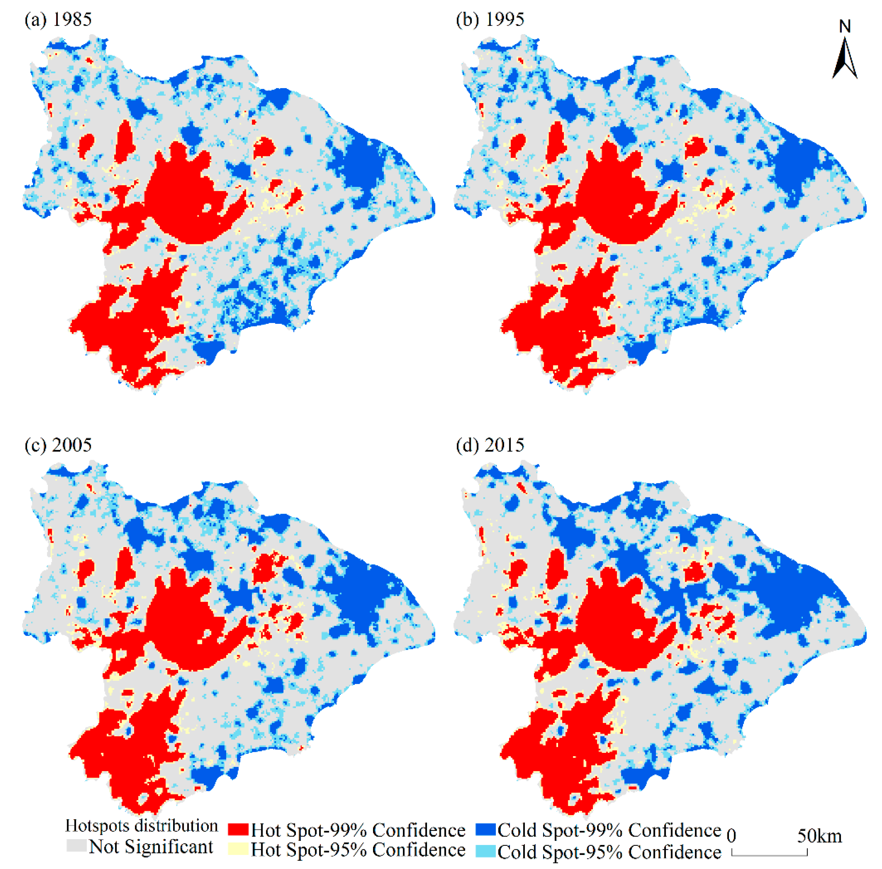
3.3. Hotspots Identification of Habitat Quality

The spatial hotspots distribution of HQ in the TLB is shown in Figure 6. The spatial distribution of HQ in the TLB showed a pattern of “hot in the west and cold in the east”. The hotspots area was mainly located in the west and south, clustered around lakes and mountains. Mountains and waters are important habitat types where human disturbance is relatively small, thus the HQ was generally higher. The cold spots areas were mainly distributed in the north and east of the TLB. These areas were flat terrain, where a large number of towns, villages, and roads and other construction land were distributed in. Due to the strong interference of human activities, the HQ in these areas were lower. The distribution of sub-cold spots and sub-hotspots were not obvious in the TLB. From 1985 to 2015, the hotspots area showed a decreasing trend, and was more obvious in the southwest mountainous area, while the cold spots area showed an increasing trend, and the northern and eastern areas were more visible. It is worth noting that the surrounding area of the water body, especially around the Taihu Lake, had a marked increase in the cold spots area, indicating that the source of habitat threats around Taihu Lake had increased.

4. Discussion

4.1. Habitat Degradation Change Associated with LUCC

Habitat degradation can be used to predict the potential for future damage to the ecological environment and the decline in HQ. It reflects the extent to which the grid unit of the landscape type is affected by threat factors. The higher the value, the greater the impact of threat factors on the grid unit, and the higher the degree of habitat degradation [12]. The spatial distribution and ratio of habitat degradation of TLB are shown in Figure 7. With time, the low degradation area ratio was decreased from 12.36% in 1985 to 9.53% in 2015, while the high degradation area ratio had increased significantly, from 3.79% in 1985 to 9.03% in 2015. This indicated that the threats sources and their accessibility has increased and the TLB is at risk of habitat degradation. In this study, we conducted construction land, farmland, unutilized land, and roads as threats factors, from the previous analyses of land-use changes, construction land, i.e., non-habitat type had increased from 9.67 % in 1985 to 26.28 in 2015, meanwhile, with the rapid development of urbanization, all kinds of roads in the study area increased rapidly, greatly increasing the road threats and their accessibility, as a result.

Regions with high degradation were mainly located near big cities and along roads. In 1985 and 1995, highly degraded areas were concentrated in urban areas and distributed around cities in a circular shape. By 2005 and 2015, with the increasing density of roads, the areas with a high degradation were linearly distributed around roads and gradually connected with the degraded areas around cities. In addition, the degradation degree around the watershed has been increasing, especially the area with a low degradation in the Taihu Lake has been shrinking significantly, which indicated that the impact of human activities on the watershed has been deepening. These findings supported the previous studies that demonstrated that urbanization has had a significant and extensive impact on the local biodiversity [36,62].

4.2. Linking Habitat Quality, Land Use, and Human Well-Being

Regional HQ directly affects human livelihoods and well-being, previous studies have indicated that urbanization has had major and widespread impacts on the native biodiversity, and has thus caused the loss of HQ [74,75]. With the development of the social economy and the growth of population, the contradiction between human and land has intensified [2,76], and the impact of human disturbance on habitats has been growing, along with changes in land use, this interaction is closely related to human well-being [77]. In order to improve human well-being and achieve sustainable development, we need to comprehensively understand and evaluate the health of complex ecosystems, in various ways [51]. To this end, the InVEST model provides us with good research methods and perspectives [11,21].

This study indicated that the HQ was mainly influenced by land-use change. A great deal of farmland was occupied by construction land, resulting in the loss and fragmentation of habitats, and in turn, leading to HQ reduction in the region. One of the main reasons for the decrease is that farmland has been transferred into construction land, under the background of rapid urban development, which is consistent with previous studies in other areas at home and abroad, such as Beijing city [25], Shule river basin [78], Yellow river delta [79], Northeast China [64], the Po river delta [2], Lake Michigan tributaries [80], and Bharathapuzha river basin [77]. This indicates that HQ decline caused by land-use change is a common phenomenon and has aroused widespread attention. In terms of landscape pattern, TLB had undergone strong landscape fragmentation during the study period, the landscape pattern became increasingly diverse, irregular, fragmented, and isolated; similar situations have been reported in related studies [62,64,65,66,67,81]. In the process of urbanization, the rapid increase of construction land threatens the surrounding habitats, resulting in an increased habitat fragmentation and poor connectivity, which ultimately leads to a decline in HQ. Landscape level index in this study showed that fragmentation, aggregation, and heterogeneity were closely related to the decline of HQ, which has been proven to be a major factor of HQ decline [64,82]. Other scholars have showed evidence of HQ decline in the Jiangsu section of the TLB and the Changzhou city [6,39], our research further enriches the habitat-degradation and HQ study in the TLB.

4.3. Policy Implication

The social and economic development of the TLB is ever growing and land use is constantly changing, as a result, the decline of HQ in TLB is becoming increasingly prominent. To improve the HQ in TLB and achieve a sustainable development, it is suggested that the corresponding scientific land management strategies should be implemented in a targeted manner, according to the regional differences in HQ.

(1) In the south, the west, and the central part of the basin, the land-use types are mainly forestland and water, which are important habitat gathering area with good or relatively good HQ. For these areas, occupying the ecological space for construction should be strictly controlled, and extremely important habitats and ecological spaces, for example, lakes and forestland, need to be effectively protected. In addition, for some habitats, such as bottomland and shallows, which are small and easily occupied by urban development, attention needs to be paid to their important role in maintaining biodiversity and habitat diversity. These above areas need to be strictly protected, such as by delineating the ecological conservation red line [83].

(2) In areas with moderate HQ, where farmland is the main land-use type. As the core carrier of agriculture space, farmland (including paddy fields and dry land) must be effectively protected. HQ of dry land has been affected to a lesser degree, so it is necessary to avoid increasing any threat to it. The encroachment of large areas of paddy fields by construction land needs to be reduced in the future. It is recommended to stabilize the agricultural space and reduce the loss of important farmland resources by strictly controlling farmland transition. For instance, delineating the red line of permanent basic farmland protection to strengthen the construction of farmland ecosystem [84].

(3) In the northern, eastern, and southern urban areas of the basin, construction land with poor or relatively poor HQ is dominant. It is necessary to optimize the allocation of land use on the premise of understanding the HQ and the risk of degradation [85,86]. Identification of urban growth boundary is regarded as an effective way to control disorderly urban sprawl, our results can provide an important basis for the urban planning process. Specifically, planners should select districts with lower HQ as construction land, and the urban growth boundary can be determined on the basis of a given area of construction land requirements. Considering the diverse future land demand scenarios, different urban growth boundaries can be developed.

4.4. Research Limitations and Future Prospects

This study used the InVEST model to explore the temporal and spatial variation of HQ in the TLB, over the past 30 years, which was helpful to deepen the understanding of the HQ of TLB on the basis of the existing literature, thus, broadening the horizon of HQ research in the TLB. However, due to the limited data obtained in this study, it will be necessary to continue to supplement the following aspects in the future.

(1) How to set input parameters of the HQ model more rationality requires further study, such as the maximum influence distance, the threat-source weight, and the habitat sensitivity, which have certain subjectivity and affect the HQ evaluation to some extent. In this study, the HQ was calculated based on the area threat sources of LULC, and the linear threat sources of railway and highway construction. The impact of non-stationary point threat-sources, such as pollutant emissions, was not studied. In the future, it is necessary to strengthen the collection of point threat-sources data and consider the impact of specific human activities on HQ, to further supplement and optimize the model parameters, in order to obtain more accurate analysis results [6,75].

(2) The InVEST model integrates a variety of ES assessment models. Some related studies have been carried out on some ES functions in the TLB, such as water production [43], carbon storage [44], crop production [46], etc. In the future, the combination of the HQ module and other ES function assessment modules can be further considered. Based on this model, integrated ES in TLB can be analyzed. The change will provide support for ecological security and a sustainable development.

(3) In addition, there are some other factors that HQ module of the InVEST model tool does not yet consider and need to be strengthened. For instance, the socio-ecological interaction based on the stakeholder perspective needs to be taken into account, as changes in HQ actually reflect the stakeholder’s trade-offs in ES. It is important to understand the behavior and attitude of stakeholders when carrying out ecological environmental protection. Then, we can optimize human activities and promote the harmonious development of human–land relationship. Beyond this, climate change and species information (especially invasive species) are quite sensitive to habitat loss and fragmentation. Therefore, the changes of HQ can be more comprehensively understood by combining their impact.

5. Conclusions

Taking the TLB as an example, this study investigated the HQ changes in TLB associated with land-use change between 1985 and 2015, based on the ArcGIS platform and the InVEST model, the hotspots and causes of the HQ were revealed. This will be helpful for enriching the study of temporal and spatial changes of HQ in TLB, and it also has a positive reference for ecological security construction and pattern optimization in TLB. It was conducted that, (1) the land-use changed dramatically during the past 30 years—among six land-use types, the change was dominated by the continuous increase of construction land and a sharp decrease of farmland; the land use transferred mainly from farmland to construction land. Urban land expansion in the process of urbanization in TLB usually occurred on farmland, especially around big cities, including Shanghai, Suzhou, Wuxi, and Changzhou. (2) The landscape pattern had changed significantly with the LUCC, landscape level index indicated that the landscape pattern in the TLB became increasingly more diverse, irregular, and isolated. It turned out that the TLB had undergone strong landscape fragmentation during the study period. (3) The HQ of the TLB showed a downward trend during 30 years, the hotspots area was mainly clustered around lakes and mountains, while the cold spots areas were mainly distributed around cities and roads. (4) This study provides the longtime land-use change, landscape pattern, and HQ information of the TLB, which would be helpful to minimize the degradation of ES in future environmental conservation.

References

1. Mace, G.M.; Norris, K.; Fitter, A.H. Biodiversity and ecosystem services: A multilayered relationship. Trends Ecol. Evol. 2012, 27, 19–26. [Google Scholar] [CrossRef] [PubMed]
2. Gaglio, M.; Aschonitis, V.G.; Gissi, E.; Castaldelli, G.; Fano, E.A. Land use change effects on ecosystem services of river deltas and coastal wetlands: Case study in Volano–Mesola–Goro in Po river delta (Italy). Wetl. Ecol. Manag. 2017, 25, 67–86. [Google Scholar] [CrossRef]
3. Rands, M.R.W.; Adams, W.M.; Bennun, L.; Butchart, S.H.M.; Clements, A.; Coomes, D.; Entwistle, A.; Hodge, I.; Kapos, V.; Scharlemann, J.P.W.; et al. Biodiversity Conservation: Challenges Beyond 2010. Science 2010, 329, 1298–1303. [Google Scholar] [CrossRef] [PubMed] [Green Version]
4. Wu, J.-S.; Cao, Q.-W.; Shi, S.-Q.; Huang, X.-L.; Lu, Z.-Q. Spatio-temporal variability of habitat quality in Beijing-Tianjin-Hebei Area based on land use change. Ying Yong Sheng Tai Xue Bao = J. Appl. Ecol. 2015, 26, 3457–3466. [Google Scholar] [CrossRef]
5. Liu, D.; Liang, X.; Chen, H.; Zhang, H.; Mao, N. A Quantitative Assessment of Comprehensive Ecological Risk for a Loess Erosion Gully: A Case Study of Dujiashi Gully, Northern Shaanxi Province, China. Sustainability 2018, 10, 3239. [Google Scholar] [CrossRef]
6. Gao, Y.; Ma, L.; Liu, J.X.; Zhuang, Z.Z.; Huang, Q.H.; Li, M.C. Constructing Ecological Networks Based on Habitat Quality Assessment: A Case Study of Changzhou, China. Sci. Rep. 2017, 7, 11. [Google Scholar] [CrossRef] [PubMed]
7. Carvalho, F.; Carvalho, R.; Mira, A.; Beja, P. Assessing landscape functional connectivity in a forest carnivore using path selection functions. Landsc. Ecol. 2016, 31, 1021–1036. [Google Scholar] [CrossRef]
8. Fuller, T.; Sanchez-Cordero, V.; Illoldi-Rangel, P.; Linaje, M.; Sarkar, S. The cost of postponing biodiversity conservation in Mexico. Biol. Conserv. 2007, 134, 593–600. [Google Scholar] [CrossRef]
9. Long, H.L.; Liu, Y.Q.; Hou, X.G.; Li, T.T.; Li, Y.R. Effects of land use transitions due to rapid urbanization on ecosystem services: Implications for urban planning in the new developing area of China. Habitat Int. 2014, 44, 536–544. [Google Scholar] [CrossRef]
10. Hooper, D.U.; Chapin, F.S.; Ewel, J.J.; Hector, A.; Inchausti, P.; Lavorel, S.; Lawton, J.H.; Lodge, D.M.; Loreau, M.; Naeem, S.; et al. Effects of biodiversity on ecosystem functioning: A consensus of current knowledge. Ecol. Monogr. 2005, 75, 3–35. [Google Scholar] [CrossRef]
11. Terrado, M.; Sabater, S.; Chaplin-Kramer, B.; Mandle, L.; Ziv, G.; Acuna, V. Model development for the assessment of terrestrial and aquatic habitat quality in conservation planning. Sci. Total Environ. 2016, 540, 63–70. [Google Scholar] [CrossRef] [PubMed] [Green Version]
12. Sharp, R.; Tallis, H.T.; Ricketts, T.; Guerry, A.D.; Wood, S.A.; Chaplin-Kramer, R.; Nelson, E.; Ennaanay, D.; Wolny, S.; Olwero, N.; et al. InVEST 3.7.0.post9+ug.h12fcefd18548 User’s Guide; The Natural Capital Project, Stanford University, University of Minnesota, The Nature Conservancy, and World Wildlife Fund, 2018; Available online: http://releases.naturalcapitalproject.org/invest-userguide/latest/InVEST_3.7.0.post10+h2ce175de3cea_Documentation.pdf (accessed on 4 May 2019).
13. McKinney, M.L. Urbanization, biodiversity, and conservation. Bioscience 2002, 52, 883–890. [Google Scholar] [CrossRef]
14. Peng, J.; Pan, Y.; Liu, Y.; Zhao, H.; Wang, Y. Linking ecological degradation risk to identify ecological security patterns in a rapidly urbanizing landscape. Habitat Int. 2018, 71, 110–124. [Google Scholar] [CrossRef]
15. Cotter, M.; Häuser, I.; Harich, F.K.; He, P.; Sauerborn, J.; Treydte, A.C.; Martin, K.; Cadisch, G. Biodiversity and ecosystem services−A case study for the assessment of multiple species and functional diversity levels in a cultural landscape. Ecol. Indic. 2017, 75, 111–117. [Google Scholar] [CrossRef]
16. Parkes, M. Personal commentaries on “Ecosystems and human well-being: Health synthesis—A report of the Millennium Ecosystem Assessment”. Ecohealth 2006, 3, 136–140. [Google Scholar] [CrossRef]
17. Zhao, G.; Liu, J.; Kuang, W.; Ouyang, Z. Disturbance impacts of land use change on biodiversity conservation priority areas across China during 1990-2010. Acta Geogr. Sin. 2014, 69, 1640–1650. [Google Scholar] [CrossRef]
18. Liu, Y.; Huang, X.; Yang, H.; Zhong, T. Environmental effects of land-use/cover change caused by urbanization and policies in Southwest China Karst area—A case study of Guiyang. Habitat Int. 2014, 44, 339–348. [Google Scholar] [CrossRef]
19. Guo, Z.; Zhang, L.; Li, Y. Increased Dependence of Humans on Ecosystem Services and Biodiversity. PLoS ONE 2010, 5, e13113. [Google Scholar] [CrossRef] [PubMed]
20. Petrosillo, I.; Zaccarelli, N.; Semeraro, T.; Zurlini, G. The effectiveness of different conservation policies on the security of natural capital. Landsc. Urban Plan. 2009, 89, 49–56. [Google Scholar] [CrossRef]
21. Romero-Calcerrada, R.; Luque, S. Habitat quality assessment using Weights-of-Evidence based GIS modelling: The case of Picoides tridactylus as species indicator of the biodiversity value of the Finnish forest. Ecol. Model. 2006, 196, 62–76. [Google Scholar] [CrossRef]
22. Ahrends, A.; Hollingsworth, P.M.; Ziegler, A.D.; Fox, J.M.; Chen, H.F.; Su, Y.F.; Xu, J.C. Current trends of rubber plantation expansion may threaten biodiversity and livelihoods. Glob. Environ. Chang. 2015, 34, 48–58. [Google Scholar] [CrossRef]
23. Donald, P.F.; Green, R.E.; Heath, M.F. Agricultural intensification and the collapse of Europe’s farmland bird populations. Proc. R. Soc. Lond. Ser. B Biol. Sci. 2001, 268, 25–29. [Google Scholar] [CrossRef] [PubMed]
24. Otto, C.R.V.; Roth, C.L.; Carlson, B.L.; Smart, M.D. Land-use change reduces habitat suitability for supporting managed honey bee colonies in the Northern Great Plains. Proc. Natl. Acad. Sci. USA 2016, 113, 10430–10435. [Google Scholar] [CrossRef] [PubMed] [Green Version]
25. Chen, Y.; Qiao, F.; Jiang, L. Effects of Land Use Pattern Change on Regional Scale Habitat Quality Based on InVEST Modela Case Study in Beijing. Acta Sci. Nat. Univ. Pekin. 2016, 52, 553–562. [Google Scholar] [CrossRef]
26. He, J.; Huang, J.; Li, C. The evaluation for the impact of land use change on habitat quality: A joint contribution of cellular automata scenario simulation and habitat quality assessment model. Ecol. Model. 2017, 366, 58–67. [Google Scholar] [CrossRef]
27. Yan, S.; Wang, X.; Cai, Y.; Li, C.; Yan, R.; Cui, G.; Yang, Z. An Integrated Investigation of Spatiotemporal Habitat Quality Dynamics and Driving Forces in the Upper Basin of Miyun Reservoir, North China. sustainability 2018, 10, 1–17. [Google Scholar] [CrossRef]
28. Ochoa, V.; Urbina-Cardona, N. Tools for spatially modeling ecosystem services: Publication trends, conceptual reflections and future challenges. Ecosyst. Serv. 2017, 26, 155–169. [Google Scholar] [CrossRef]
29. Huang, L.; Liao, F.H.; Lohse, K.A.; Larson, D.M.; Fragkias, M.; Lybecker, D.L.; Baxter, C.V. Land conservation can mitigate freshwater ecosystem services degradation due to climate change in a semiarid catchment: The case of the Portneuf River catchment, Idaho, USA. Sci. Total Environ. 2019, 651, 1796–1809. [Google Scholar] [CrossRef]
30. Meisch, C.; Schirpke, U.; Huber, L.; Rudisser, J.; Tappeiner, U. Assessing Freshwater Provision and Consumption in the Alpine Space Applying the Ecosystem Service Concept. Sustainability 2019, 11, 16. [Google Scholar] [CrossRef]
31. Xu, X.; Yang, G.; Tan, Y.; Liu, J.; Hu, H. Ecosystem services trade-offs and determinants in China’s Yangtze River Economic Belt from 2000 to 2015. Sci. Total Environ. 2018, 634, 1601–1614. [Google Scholar] [CrossRef]
32. Polasky, S.; Nelson, E.; Pennington, D.; Johnson, K.A. The Impact of Land-Use Change on Ecosystem Services, Biodiversity and Returns to Landowners: A Case Study in the State of Minnesota. Environ. Resour. Econ. 2011, 48, 219–242. [Google Scholar] [CrossRef]
33. Leh, M.D.K.; Matlock, M.D.; Cummings, E.C.; Nalley, L.L. Quantifying and mapping multiple ecosystem services change in West Africa. Agric. Ecosyst. Environ. 2013, 165, 6–18. [Google Scholar] [CrossRef]
34. Baral, H.; Keenan, R.J.; Sharma, S.K.; Stork, N.E.; Kasel, S. Spatial assessment and mapping of biodiversity and conservation priorities in a heavily modified and fragmented production landscape in north-central Victoria, Australia. Ecol. Indic. 2014, 36, 552–562. [Google Scholar] [CrossRef]
35. Wu, C.F.; Lin, Y.P.; Chiang, L.C.; Huang, T. Assessing highway’s impacts on landscape patterns and ecosystem services: A case study in Puli Township, Taiwan. Landsc. Urban Plan. 2014, 128, 60–71. [Google Scholar] [CrossRef]
36. Li, F.; Wang, L.; Chen, Z.; Clarke, K.C.; Li, M.; Jiang, P. Extending the SLEUTH model to integrate habitat quality into urban growth simulation. J. Environ. Manag. 2018, 217, 486–498. [Google Scholar] [CrossRef] [PubMed] [Green Version]
37. Schleupner, C.; Link, P.M. Potential impacts on important bird habitats in Eiderstedt (Schleswig-Holstein) caused by agricultural land use changes. Appl. Geogr. 2008, 28, 237–247. [Google Scholar] [CrossRef]
38. Wang, Y.T.; Li, X.; Sun, M.X.; Yu, H.J. Managing urban ecological land as properties: Conceptual model, public perceptions, and willingness to pay. Resour. Conserv. Recycl. 2018, 133, 21–29. [Google Scholar] [CrossRef]
39. Ai, J.Y.; Sun, X.; Feng, L.; Li, Y.F.; Zhu, X.D. Analyzing the spatial patterns and drivers of ecosystem services in rapidly urbanizing Taihu Lake Basin of China. Front. Earth Sci. 2015, 9, 531–545. [Google Scholar] [CrossRef]
40. Xu, X.B.; Yang, G.S.; Tan, Y.; Tang, X.G.; Jiang, H.; Sun, X.X.; Zhuang, Q.L.; Li, H.P. Impacts of land use changes on net ecosystem production in the Taihu Lake Basin of China from 1985 to 2010. J. Geophys. Res. Biogeosci. 2017, 122, 690–707. [Google Scholar] [CrossRef]
41. Li, J.; Jiang, H.; Bai, Y.; Alatalo, J.M.; Li, X.; Jiang, H.; Liu, G.; Xu, J. Indicators for spatial–temporal comparisons of ecosystem service status between regions: A case study of the Taihu River Basin, China. Ecol. Indic. 2016, 60, 1008–1016. [Google Scholar] [CrossRef]
42. Sun, X.; Xiong, S.; Zhu, X.; Zhu, X.; Li, Y.; Li, B.L. A new indices system for evaluating ecological-economic-social performances of wetland restorations and its application to Taihu Lake Basin, China. Ecol. Model. 2015, 295, 216–226. [Google Scholar] [CrossRef]
43. Guo, L. Doing battle with the green monster of Taihu Lake. Science 2007, 317, 1166. [Google Scholar] [CrossRef] [PubMed]
44. Wang, G.X.; Zhang, L.M.; Zhuang, Q.L.; Yu, D.S.; Shi, X.Z.; Xing, S.H.; Xiong, D.Z.; Liu, Y.L. Quantification of the soil organic carbon balance in the Tai-Lake paddy soils of China. Soil Tillage Res. 2016, 155, 95–106. [Google Scholar] [CrossRef]
45. Yin, Y.X.; Xu, Y.P.; Chen, Y. Relationship between flood/drought disasters and ENSO from 1857 to 2003 in the Taihu Lake basin, China. Quat. Int. 2009, 208, 93–101. [Google Scholar] [CrossRef]
46. Liu, G.L.; Zhang, L.C.; Zhang, Q.; Musyimi, Z. The response of grain production to changes in quantity and quality of cropland in Yangtze River Delta, China. J. Sci. Food Agric. 2015, 95, 480–489. [Google Scholar] [CrossRef] [PubMed]
47. Xu, X.B.; Yang, G.S.; Tan, Y.; Zhuang, Q.L.; Li, H.P.; Wan, R.R.; Su, W.Z.; Zhang, J. Ecological risk assessment of ecosystem services in the Taihu Lake Basin of China from 1985 to 2020. Sci. Total Environ. 2016, 554, 7–16. [Google Scholar] [CrossRef] [PubMed]
48. Qiao, X.N.; Gu, Y.Y.; Zou, C.X.; Xu, D.L.; Wang, L.; Ye, X.; Yang, Y.; Huang, X.F. Temporal variation and spatial scale dependency of the trade-offs and synergies among multiple ecosystem services in the Taihu Lake Basin of China. Sci. Total Environ. 2019, 651, 218–229. [Google Scholar] [CrossRef] [PubMed]
49. Liu, H.; Cai, Y.; Yu, M.; Gong, L.; An, S. Assessment of river habitat quality in Yixing district of Taihu Lake basin. Chin. J. Ecol. 2012, 31, 1288–1295. [Google Scholar] [CrossRef]
50. Gaglio, M.; Lanzoni, M.; Nobili, G.; Viviani, D.; Castaldelli, G.; Fano, E.A. Ecosystem services approach for sustainable governance in a brackish water lagoon used for aquaculture. J. Environ. Plan. Manag. 2019, 1–24. [Google Scholar] [CrossRef]
51. Adger, W.N.; Adams, H.; Kay, S.; Nicholls, R.J.; Hutton, C.W.; Hanson, S.E.; Rahman, M.M.; Salehin, M. Ecosystem Services, Well-Being and Deltas: Current Knowledge and Understanding. Ecosyst. Serv. Well-Being Deltas 2018, 1. [Google Scholar] [CrossRef]
52. Fu, B.J.; Wang, S.; Su, C.H.; Forsius, M. Linking ecosystem processes and ecosystem services. Curr. Opin. Environ. Sustain. 2013, 5, 4–10. [Google Scholar] [CrossRef]
53. Wang, C.; Bi, J. TMDL development for the Taihu Lake’s influent rivers, China using variable daily load expressions. Stoch. Environ. Res. Risk Assess. 2016, 30, 1–11. [Google Scholar] [CrossRef]
54. Qiao, X.M.; Gu, Y.Y.; Zou, C.X.; Wang, L.; Luo, J.H.; Huang, X.F. Trade-offs and Synergies of Ecosystem Services in the Taihu Lake Basin of China. Chin. Geogr. Sci. 2018, 28, 86–99. [Google Scholar] [CrossRef] [Green Version]
55. Taihu Basin Authority of Ministry of Water Resources. Taihu Basin and Southeast Rivers Water Resource Bulletin. Available online: http://www.tba.gov.cn/contents/44/14716.html (accessed on 4 May 2019).
56. Su, W.Z.; Gu, C.L.; Yang, G.S.; Chen, S.; Zhen, F. Measuring the impact of urban sprawl on natural landscape pattern of the Western Taihu Lake watershed, China. Landsc. Urban Plan. 2010, 95, 61–67. [Google Scholar] [CrossRef]
57. Zhou, S.; Du, A.; Bai, M. Application of the environmental Gini coefficient in allocating water governance responsibilities: A case study in Taihu Lake Basin, China. Water Sci. Technol. 2015, 71, 1047–1055. [Google Scholar] [CrossRef]
58. Liu, J.Y.; Zhang, Z.X.; Xu, X.L.; Kuang, W.H.; Zhou, W.C.; Zhang, S.W.; Li, R.D.; Yan, C.Z.; Yu, D.S.; Wu, S.X.; et al. Spatial patterns and driving forces of land use change in China during the early 21st century. J. Geogr. Sci. 2010, 20, 483–494. [Google Scholar] [CrossRef]
59. Xu, X.L.; Pang, Z.G.; Wang, X.F. Spatial-Temporal Pattern Analysis of Land Use/Cover; Scientific and Technical Documentation Press: Beijing, China, 2014. [Google Scholar]
60. Liu, J.Y.; Zhang, Z.X.; Zhuang, D.F.; Zhang, S.W.; Li, X.B. Remote Sensing Information Study of Land Use Change in China in 1990s; Sciences Press: Beijing, China, 2005. [Google Scholar]
61. Ye, G.; Su, W.; Chen, W. The Elevation Characteristics Variation of Urban and Rural Construction Land Expansion in Taihu Lake Basin. J. Nat. Resour. 2015, 30, 938–950. [Google Scholar] [CrossRef]
62. Deng, Y.; Jiang, W.; Wang, W.; Lu, J.; Chen, K. Urban expansion led to the degradation of habitat quality in the Beijing-Tianjin-Hebei Area. Acta Ecol. Sin. 2018, 38, 4516–4525. [Google Scholar] [CrossRef]
63. Lin, Y.-P.; Lin, W.-C.; Wang, Y.-C.; Lien, W.-Y.; Huang, T.; Hsu, C.-C.; Schmeller, D.S.; Crossman, N.D. Systematically designating conservation areas for protecting habitat quality and multiple ecosystem services. Environ. Model. Softw. 2017, 90, 126–146. [Google Scholar] [CrossRef]
64. Dai, L.; Li, S.; Lewis, B.J.; Wu, J.; Yu, D.; Zhou, W.; Zhou, L.; Wu, S. The influence of land use change on the spatial–temporal variability of habitat quality between 1990 and 2010 in Northeast China. J. For. Res. 2018, 1–10. [Google Scholar] [CrossRef]
65. Liu, Z.; Tang, L.; Qiu, Q.; Xiao, L.; Xu, T.; Yang, L. Temporal and spatial changes in habitat quality based on land-use change in Fujian Province. Acta Ecol. Sin. 2017, 37, 4538–4548. [Google Scholar] [CrossRef]
66. Feng, Y.J.; Liu, Y.; Tong, X.H. Spatiotemporal variation of landscape patterns and their spatial determinants in Shanghai, China. Ecol. Indic. 2018, 87, 22–32. [Google Scholar] [CrossRef]
67. Szilassi, P.; Bata, T.; Szabo, S.; Czucz, B.; Molnar, Z.; Mezosi, G. The link between landscape pattern and vegetation naturalness on a regional scale. Ecol. Indic. 2017, 81, 252–259. [Google Scholar] [CrossRef] [Green Version]
68. McGarigal, K. FRAGSTATS v4: Spatial Pattern Analysis Program for Categorical and Continuous Maps. Computer software program produced by the authors at the University of Massachusetts, Amherst. Available online: http://www.umass.edu/landeco/research/fragstats/fragstats.html (accessed on 4 May 2019).
69. Hou, Y.; Li, B.; Muller, F.; Chen, W.P. Ecosystem services of human-dominated watersheds and land use influences: A case study from the Dianchi Lake watershed in China. Environ. Monit. Assess. 2016, 188, 652. [Google Scholar] [CrossRef] [PubMed]
70. Ou, W.; Zhang, L.; Tao, Y.; Guo, J. A land-cover-based approach to assessing the spatio-temporal dynamics of ecosystem health in the Yangtze River Delta region. China Popul. Resour. Environ. 2018, 28, 84–92. [Google Scholar] [CrossRef]
71. Zhang, D.; Sun, X.; Yuan, X.; Liu, F.; Guo, H.; Xu, Y.; Li, B. Land use change and its impact on habitat quality in Lake Nansi Basin from 1980 to 2015. J. Lake Sci. 2018, 30, 349–357. [Google Scholar] [CrossRef]
72. Getis, A.; Ord, J.K. The Analysis of Spatial Association by Use of Distance Statistics. Geogr. Anal. 1992, 24, 189–206. [Google Scholar] [CrossRef]
73. Li, Y.J.; Zhang, L.W.; Yan, J.P.; Wang, P.T.; Hu, N.K.; Cheng, W.; Fu, B.J. Mapping the hotspots and coldspots of ecosystem services in conservation priority setting. J. Geogr. Sci. 2017, 27, 681–696. [Google Scholar] [CrossRef]
74. Li, X.; Hou, X.; Song, Y.; Shan, K.; Zhu, S.; Yu, X.; Mo, X. Assessing Changes of Habitat Quality for Shorebirds in Stopover Sites: A Case Study in Yellow River Delta, China. Wetlands 2018, 39, 67–77. [Google Scholar] [CrossRef]
75. Jie, G.; Feng, L.; Hui, G.; Zhou, C.; Zhang, X. The impact of land-use change on water-related ecosystem services: A study of the Guishui River Basin, Beijing, China. J. Clean. Prod. 2015, 163, S148–S155. [Google Scholar] [CrossRef]
76. Lu, X.L.; Zhou, Y.Y.; Liu, Y.L.; Le Page, Y. The role of protected areas in land use/land cover change and the carbon cycle in the conterminous United States. Glob. Chang. Biol. 2018, 24, 617–630. [Google Scholar] [CrossRef] [PubMed]
77. John, J.; Chithra, N.R.; Thampi, S.G. Prediction of land use/cover change in the Bharathapuzha river basin, India using geospatial techniques. Environ. Monit. Assess. 2019, 191, 15. [Google Scholar] [CrossRef] [PubMed]
78. Ma, L.B.; Bo, J.; Li, X.Y.; Fang, F.; Cheng, W.J. Identifying key landscape pattern indices influencing the ecological security of inland river basin: The middle and lower reaches of Shule River Basin as an example. Sci. Total Environ. 2019, 674, 424–438. [Google Scholar] [CrossRef] [PubMed]
79. Yang, W.; Jin, Y.; Sun, T.; Yang, Z.; Cai, Y.; Yi, Y. Trade-offs among ecosystem services in coastal wetlands under the effects of reclamation activities. Ecol. Indic. 2017, 92, 354–366. [Google Scholar] [CrossRef]
80. Brumm, K.J.; Jonas, J.L.; Prichard, C.G.; Watson, N.M.; Pangle, K.L. Land cover influences on juvenile Rainbow Trout diet composition and condition in Lake Michigan tributaries. Ecol. Freshw. Fish 2019, 28, 11–19. [Google Scholar] [CrossRef]
81. Su, S.; Rui, X.; Jiang, Z.; Yuan, Z. Characterizing landscape pattern and ecosystem service value changes for urbanization impacts at an eco-regional scale. Appl. Geogr. 2012, 34, 295–305. [Google Scholar] [CrossRef]
82. Boswell, G.P.; Britton, N.F.; Franks, N.R. Habitat fragmentation, percolation theory and the conservation of a keystone species. Proc. R. Soc. Lond. Ser. B Biol. Sci. 1998, 265, 1921–1925. [Google Scholar] [CrossRef]
83. Gao, J. How China will protect one-quarter of its land. Nature 2019, 569, 457. [Google Scholar] [CrossRef]
84. Su, W.; Ru, J.; Yang, G. Modelling stormwater management based on infiltration capacity of land use in the watershed scale. Acta Geogr. Sin. 2019, 74, 948–961. [Google Scholar] [CrossRef]
85. Ren, C.F.; Li, Z.H.; Zhang, H.B. Integrated multi-objective stochastic fuzzy programming and AHP method for agricultural water and land optimization allocation under multiple uncertainties. J. Clean. Prod. 2019, 210, 12–24. [Google Scholar] [CrossRef]
86. Singh, A. Optimal allocation of water and land resources for maximizing the farm income and minimizing the irrigation-induced environmental problems. Stoch. Environ. Res. Risk Assess. 2017, 31, 1147–1154. [Google Scholar] [CrossRef]
Figure 1. Location of the Taihu Lake Basin (TLB) in China.
Sustainability 11 03513 g001
Figure 2. Land-use maps of the TLB in (a) 1985, (b) 1995, (c) 2005, and (d) 2015.
Sustainability 11 03513 g002
Figure 3. Area of each land-use type of the TLB in 1985, 1995, 2005, and 2015.
Sustainability 11 03513 g003
Figure 4. Transition matrix of land-use type in the different study period (km²). (a) 1985–1995, (b) 1995–2005, (c) 2005–2015, and (d) 1985–2015 values close to the land-use type, represent the conversion area from the other land-use types.
Sustainability 11 03513 g004
Figure 5. Spatial distribution of HQ of the TLB in (a) 1985, (b) 1995, (c) 2005, and (d) 2015.
Sustainability 11 03513 g005
Figure 6. Hotspots distribution of HQ of the TLB in (a) 1985, (b) 1995, (c) 2005, and (d) 2015.
Sustainability 11 03513 g006
Figure 7. Distribution of habitat degradation of the TLB in (a) 1985, (b) 1995, (c) 2005, and (d) 2015.
Sustainability 11 03513 g007