On Soil Capability, Capacity, and Condition

Abstract

The role of soil in the existential environmental problems of declining biodiversity, climate change, water and energy security, impacting on food security has highlighted the need to link the soil functions to ecosystem services. We describe and illustrate by a limited example, the concepts and assessment of soil’s capacity measured through its capability and condition as contributors to an overall soil security framework. The framework is based on the concepts of genosoils and phenosoils. The links to other notions, such as threats to soil and soil functions are made. The framework can be potentially applied elsewhere to quantify soil changes under natural processes and human activities.

1. Introduction

There are several approaches to what soil can do functionally for humanity and/or the ecosystem. Sometimes this is called soil capability, and sometimes when the focus is on management, soil quality, soil condition, or soil health. The notion of soil quality is often defined in terms of the chemical, physical, and biological aspects of the topsoil [1]. The shift from quality to the term soil health is largely characterized by its redefinition to include biological terms [2] to capture the ecological attributes of the soil and improve communication with non-scientists. The term soil condition refers to soil changes compared to a reference state, as a function of management [3]. Soil quality is aligned with the ideas around production, while soil health attempts to expand to include the range of soil functions [4] and ecosystem services [5]. They are primarily focused on the ‘condition’ of the soil, with no explicit statement of a reference state, as implied by Sojka et al. [6], i.e., the notion of capability. Scientists have recognized a number of functions that soil can perform (a) for humanity and (b) for the general ecosystem. There is no single definition of soil functions and they are not simply a collection of intrinsic soil processes [7]. According to Lehmann and Stahr [8], earlier definitions focused on securing food production, providing and cleaning ground water, and filtering, buffering and transformation of nutrients and pollutants. Many of the earlier definitions were developed with a strong orientation toward agriculture and forestry, as demonstrated by Larson and Peirce [9]. This was followed by an expansion in thinking about soil functions to link with ecosystem functions [5,10,11]. This resulted in inclusion of soil acting as a carbon pool recognizing its contribution to climate change. The recognition of soil as a habitat for soil organisms and a genetic reserve was introduced to a broader audience outside of soil science when the European Commission focused on soil protection [12].

The role of soil in the existential environmental problems of declining biodiversity, climate change, water and energy security, impacting on food security [13] has highlighted the need to link the soil functions to ecosystem services. Both Dominati et al. 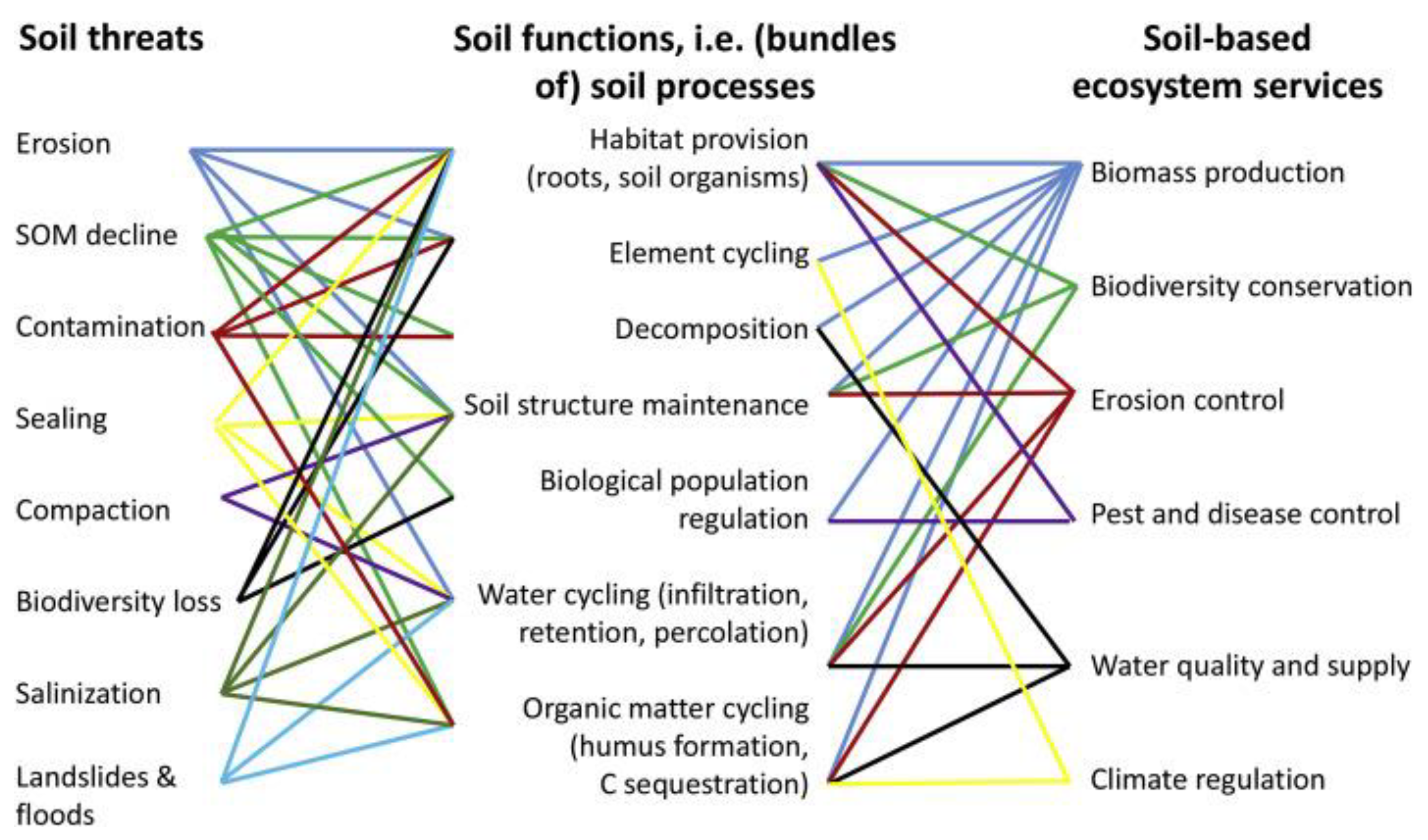[5] and Robinson [11] have clearly identified the ecosystem services and linked these to soil functions, and this is a logical way to consider interdisciplinary studies on ecosystem services [14,15]. The European Commission has also identified up to eight significant threats to soil, and McBratney et al. [3] has related these threats to the concept of soil security. The potential link between soil threats, soil functions, and soil-provided ecosystem services is illustrated in Figure 1, which is taken from Bünemann et al. [16]. In turn, soil functions have been linked to the sustainable development goals (SDGs) through ecosystem services [15]. According to Lehmann and Stahr [8], the list of soil functions in

Table 1. The seven soil functions as defined by the European Commission [12].

Number	Soil Function
1	Biomass production
2	Storing, filtering, and transformation of nutrients, substances, and water
3	Biodiversity pool, habitats, species, and genes
4	Physical and cultural environment for humans
5	Source of raw materials
6	Acting as a carbon pool
7	Archive of geological and archaeological heritage.

are applicable to agriculture, climate change, ecological systems, and urban environments.

Others try to quantify the ability of a given soil (profile, individual, areal, landscape) to perform these functions. A comprehensive set of indicators has been identified to quantify the physical, chemical, and biological properties that affect the soil condition [17] and these have often been aggregated in assessment frameworks, score cards, and kits for farmers and education [18,19]. Some of these frameworks are flexible, allowing the user to select indicators depending on the ecosystem services and management options [20], others are standardized systems targeted to particular users along with management advice [21]. There are a plethora of soil quality/health frameworks developed in Europe where there also was an attempt to develop a set focused on the assessment of the threats to soil [22], resulting in three priority indicators for each threat [23]. Dominati et al. [5] has demonstrated the use of soil properties as indicators to assess ecosystem services. Albeit, Bünemann et al. [16] stated that there are a few clear interpretation schemes of measured indicator values in relation to soil threats, soil functions, and ecosystem services. The mapping of indictors of soil quality, functions, and/or ecosystem services is becoming more feasible with the increasing adoption of spectroscopic and other remote and proximal soil sensing techniques [16,24,25]. The increasing abilities of digital soil mapping have the potential to map soil functions [26], and it is suggested that a shift in focus to digital soil assessment will focus mapping of soil functions and threats [27]. There is also the need to consider political, social, and economic aspects of soil function as a means to assess the opportunity for soil protection, i.e., a risk assessment approach [28].

It is suggested by Hatfield et al. [7] that the integration of soil functionality with the newly developed interdisciplinary soil security concept is a way to develop soil functionality and ecosystem services links. Recently, the soil security concept [3] was devised to develop a framework to consider soil function holistically and broaden the conversation beyond soil science alone. Soil security also provides a framework to quantify the magnitude and relevance of soil functions. It consists of five dimensions, capability, condition, capital, connectivity, and codification.

(a) Capability and (b) Condition attempt to measure the biophysical ability of a soil to carry out a function, while the other dimensions attempt to make and measure non-biophysical statements and estimates about whether a soil can continue to support that function or range of functions through.

(c) The Capital value of soil affords the production of human-demanded function and the attendant ecosystem services. The larger this value, the greater the potential for capturing the attention of those using soil functions and services and presumably the greater the potential for recognizing the importance of soil in society, policy, and the economy. (d) The Connectivity between soil and those who wish to use its products and services. The larger this connection the greater the potential for the society formally recognizing and protecting continued functioning.

(e) The Codification or governance of the soil is through public regulation for use or activity or private regulation through environmental sustainability accreditation and certification schemes. The greater the successful regulation, the more likely the chance of protecting the continued functioning of soil. Here we focus on (a) and (b), and suggest a way forward for their quantification and draw parallels wherever possible with other approaches. The approach proposed here is purposely generic.

2. A Generic Approach to Soil Capability, Capacity, and Condition

This kind of evaluation was to some extent conventionally done using a qualitative and later a quantitative land-evaluation approach, using decision tables or simulation modelling [29]. Later, emphasis was placed on simpler approaches using less soil information—a set of fuzzy or hard indicators [30]—and largely for some generic rather than specific biomass production function; this was the transition from land evaluation approaches to soil quality [1]. Even later, the term soil quality tended to be replaced by soil health (first coined by Acton and Gregorich [31]). Admittedly, the focus of the latter approaches was somewhat more on dynamic properties and sustainability. There is still overlap and uncertainty between these terms. Axiomatically, the more we know the more likely the quantification will be.

Let us consider evaluating some soil s for some human (or ecosystem) function f (s can be a soil profile, or the average for a soil areal depending on the context).

We can estimate capacity, condition, and capability starting with a data matrix such as this,

$$D_t=\left(\begin{array}{cc}U& Y\\ V& Z\end{array}\right)$$

U is an m by n matrix of n soil attributes observed at m soil locations (m may minimally be 1) for some soil of interest. The n soil attributes will be those that affect the function of the soil but are not readily changed by human forcing (e.g., soil clay content). This represents the capacity attributes of the soil of interest.

Y is an m by p matrix of p soil attributes observed at the same m soil locations as in U (m may minimally be 1 when it is an areal average) for the soil of interest. The p soil attributes will be those that affect the function of the soil but are readily changed by human forcing. This represents the condition attributes of the soil of interest. These conditional attributes could include undesired and desired attributes—contamination (e.g., heavy metal concentration) or agronomic (e.g., available N) attributes.

V is a q by n matrix of the same n soil attributes as in U observed at q soil locations (q may minimally be 1) for a reference soil. A reference soil is the least disturbed phenosoil (possibly the genosoil) of the soil of interest [32,33]. This represents the capacity attributes of the reference soil.

Z is an q by p matrix of the same p soil attributes as in Y observed at the same q soil locations as in V (m may minimally be 1 when it is an areal average) for the soil of interest. This represents the condition attributes of the reference soil.

Under certain circumstances, m = q. First, it may be possible to set up paired sites between the soil of interest and the reference soil; or second, when m = q = 1 this represents an areal average of the soil attributes (not a single observation or profile).

D is a m + q by n + p matrix describing the data for the assessment.

Further, we can specify, two submatrices of D

$$\begin{gathered} X_t= \left(\begin{array}{cc}U& Y\end{array}\right)=U \parallel Y, \\ {R}_t= \left(\begin{array}{cc}V& Z\end{array}\right)=V \parallel Z, \end{gathered}$$

where, $\parallel$ represents column-wise concatenation. Therefore X (m by n + p) represents the capability attributes of the soil of interest, and R (q by n + p) represents the capability attributes of the reference soil.

Recalling,

$$D_t=\left(\begin{array}{c}X\\ R\end{array}\right)=X ^ R,$$

where $^$ represents row-wise concatenation.

The capability a, is given by

$$a_f={ℂ}_f\left(X\right);$$

the capacity b, is given by

$$b_f={ℂ}_f\left(U\right);$$

and the condition c, is given by

$$c_f={ℂ}_f\left(Y\right).$$

Here, ${ℂ}_f(.)$ represents generically a (possibly nonlinear) transformation of the soil attribute data contained in the appropriate matrix to the scalar quantity. The transformation represents the ability to perform a given soil function, as outlined in the introduction. Generically, ${ℂ}_f$ would be different for each soil function f. Not all soil attributes will be given equal weight (and for some soil functions some may be unweighted). This transformation could be achieved variously, e.g., by a decision table, a combination of fuzzy indicators, or dynamic process simulation modelling.

We can calculate the differences for capability, capacity, and condition attributes relative to the reference state,

$$\begin{gathered} C_t=R- X; E_t=U- V \approx \mathbf{0};\mathrm{and} \\ {F}_t=Y- Z. \end{gathered}$$

We expect E $\approx \mathbf{0}$ (a null matrix, in this case a matrix of almost zeroes), otherwise we may need a new reference state. Most importantly, F gives a strong indication of the change in condition attributes caused by human forcings (this approximates the properties that many might ascribe to soil health or quality).

We can define other quantities, such as the following.

Differential capability d_f, is

$$d_f={ℂ}_f\left(R\right)- {ℂ}_f\left(X\right).$$

Differential capacity e_f, is

$$e_f={ℂ}_f\left(U\right)- {ℂ}_f\left(V\right).$$

Differential condition g_f, is

$$g_f={ℂ}_f\left(Y\right)- {ℂ}_f\left(Z\right).$$

Further, including the time dimension will give the associated temporal rate of change of capability, capacity, and condition. This can be estimated by the elapsed time the soil of interest has experienced different forcings (soil management) from the reference state.

The stability, resistance or buffering of capability, capacity or condition is probably most difficult to quantify because it requires a measure of the forcings themselves, not simply the temporal rate of change. The forcing could be measured by an energy or financial input; all soil can be changed if enough energy and/or economic capital is applied. After removal of the forcing, the recovery is measured by both the temporal rate and quantum of change. This is easier to estimate since it only requires temporal rates. Resistance and recovery are components of resilience [34].

Estimates of all these quantities are enhanced by having a reference soil that can be used in the calculations. Generally, the forcings are considered under various land degradation processes such as, water or wind erosion, salinization, contamination, etc. However strictly theoretically, we do not need to specify these forces of degradation. But they do indicate which soil attributes should be considered, because they may be variously affected by such forcings.

In the few paragraphs above, we have outlined a theoretical framework for quantifying aspects of capability and condition as two of the dimensions of global soil security, and for consideration in the processes of assessing changes in soil health or quality.

There are many considerations required to turn this theoretical framework into a quantitative assessment. We believe, this is possible by careful consideration. For a generic assessment we need to derive and agree upon sets of attributes that represent capacity and condition. We need to derive and agree upon appropriate ${ℂ}_f$ for each of the soil functions. Finally, we need to be able to derive reference soils at the appropriate level of taxonomic generalisation (soil classification does have its part to play). The work of Huang et al. [33] suggests a digital soil mapping approach to derive reference soil areals. A perhaps simpler, but similar approach is to derive terrons [35] and then subdivide these based on land-use history. This suggests that soil security assessment, and specifically assessments of soil condition (quality and health) should be spatially based and spatially explicit. The advantage of a spatial approach is that ameliorative operations can be actioned on the ground in known locations. The development of this approach is a surmountable and noble challenge for the wider soil science community.

3. Example

We present here a brief partial example that illustrates the key features. We acquired the approach and data from Huang et al. [33] and reinterpret the approach and results in terms of soil capability, condition, and capacity.

Huang et al. [33] recognized and mapped a number of local soil classes that could be allocated to a range of suborders of the Australian soil classification system [36]. Further, each of these local soil classes were divided into subclasses based on the degree of land management intensity by observing current and past aerial and satellite imagery. For the purpose of this paper, we concentrated on two of the classes, and within each of the classes we performed a rudimentary capability, capacity, and condition attribute analysis.

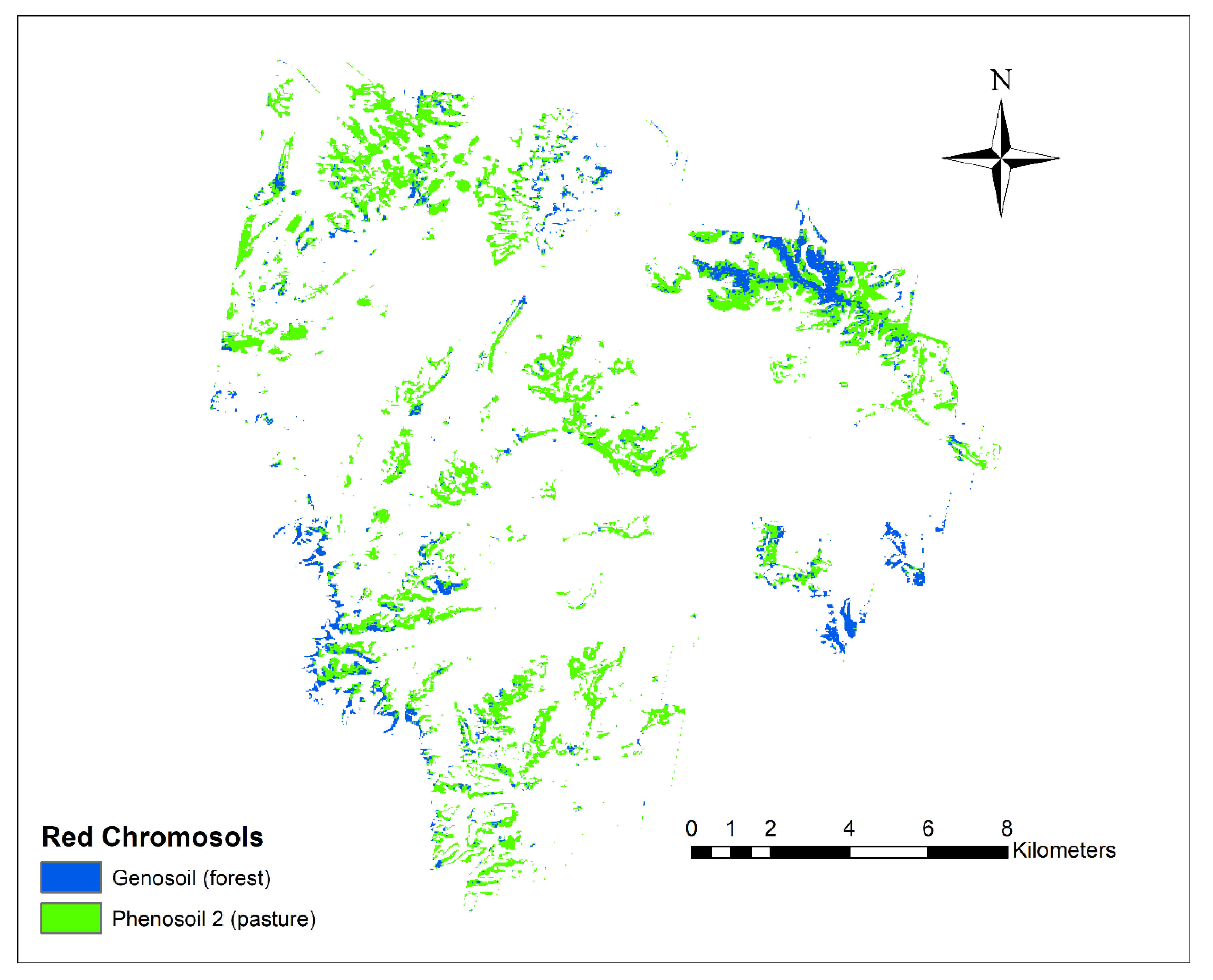
Figure 2 shows the location of Red Chromosols phenosoil 2, which are the Red Chromosols under perennial pasture management. This is the soil of interest. We compared this with Red Chromosols genosoil 1 (also shown on Figure 1), which are the least disturbed of these soils, and occur under remnant or regrowth forest. Red Chromosol genosoil 1 represents the reference soil. We have 22 observations for the reference soil and 112 for the pasture soil. Observations are from two depths, namely 0 to 10 cm and 40 to 50 cm. The soil capacity attributes are clay, silt, and sand at 0 to 10 and 40 to 50 cm, respectively (6 attributes). Using the notation from above and areal averages to describe the soil of interest and the reference soil, matrix U is then a 1 by 6 matrix (row vector) (

Table 2. Matrices of various genosoils and phenosoils for Red Chromosols and Calcarosols mapped by Huang et al. [33].

Red Chromosols	Land Cover	Capacity	Condition
Genosoil 1 (reference soil)	Forest	V = [24.0 40.4 23.8 23.0 52.2 36.7]	Z = [6.0 5.6 3.5 0.9]
Phenosoil 2	Pasture	U = [27.1 39.8 27.8 23.6 45.0 36.6]	Y = [6.1 6.2 3.3 1.1]
Change from Genosoil 1 to Phenosoil 2	Forest to Pasture	E = [3.1 −0.6 4.0 0.6 −7.2 −0.1]	F = [0.1 0.6 −0.2 0.2]
Calcarosols	Land cover	Capacity	Condition
Genosoil 1 and Phenosoil 1 (reference soil)	Forest	V = [25.4 37.4 29.4 26.2 45.1 36.4]	Z = [6.2 6.6 5.4 1.8]
Phenosoil 2	Pasture	U = [25.2 46.3 24.0 25.9 50.8 27.8]	Y = [6.8 7.5 4.9 2.0]
Phenosoil 3	Vineyard	U = [33.5 50.7 22.0 19.1 44.5 30.2]	Y = [6.9 7.7 3.9 2.1]
Change from Genosoil 1 and Phenosoil 1 to Phenosoil 2	Forest to Pasture	E = [−0.2 8.9 −5.4 −0.2 5.6 −8.7]	F = [0.7 0.9 −0.5 0.2]
Change from Genosoil 1 and Phenosoil 1 to Phenosoil 3	Forest to Vineyard	E = [8.1 13.3 −7.4 −7.1 −0.7 −6.2]	F = [0.7 1.1 −1.5 0.3]

). In this case,

U = [27.1 39.8 27.8 23.6 45.0 36.6];

where the elements are clay at 0 to 10 cm, clay at 40 to 50 cm, and likewise for silt and sand, all units of %. Similarly, for the reference soil,

V = [24.0 40.4 23.8 23.0 52.2 36.7].

Attributes of interest that are more readily affected by management include, soil pH and organic carbon, in %. These two properties were measured at the same two depths as U. Hence, matrix Y, based on 112 observations, is

Y = [6.1 6.2 3.3 1.1];

where, the elements are pH at 0 to 10 and 50 to 60 cm depth, respectively, followed by organic carbon (%) at 0 to 10 cm and 50 to 60 cm, respectively. For the reference soil, with the same attributes and in the same order,

Z = [6.0 5.6 3.5 0.9].

Recalling that matrix E = U – V

E = [3.1 −0.6 4.0 0.6 −7.2 −0.1]. The p-value, testing the hypothesis that E = 0, was calculated using the Welch Anova testing of means with unequal variances. The p-values that test changes in the soil properties (representing capability) are the following, [0.52, 0.94 0.46 0.89 0.21 0.99], where small p-values indicate means are different or E ≠ 0. In this example, we have no evidence to suggest that the means are different. The interpretation is that the capability of the Red Chromosols phenosoil 2 and genosoil 1 is similar. Or in other words genosoil 1 is of a similar texture to serve as a reference soil for phenosoil 2.

Matrix F = Y – Z;

F = [0.1 0.6 −0.2 0.2]; and the p-values are [0.24 0.0002 0.58 0.47].

The small p-value suggests a significant increase in pH (from decreased organic C and possibly from the grasses preventing deeper leaching of base cations in the subsoil. The changes indicated by F represents a time span of over 100 years, but does not indicate when or how fast the change occurred. Both the soil of interest and the reference soil have been similarly affected by climate change, and therefore that effect can be ruled out. This is an advantageous feature of the reference-state approach.

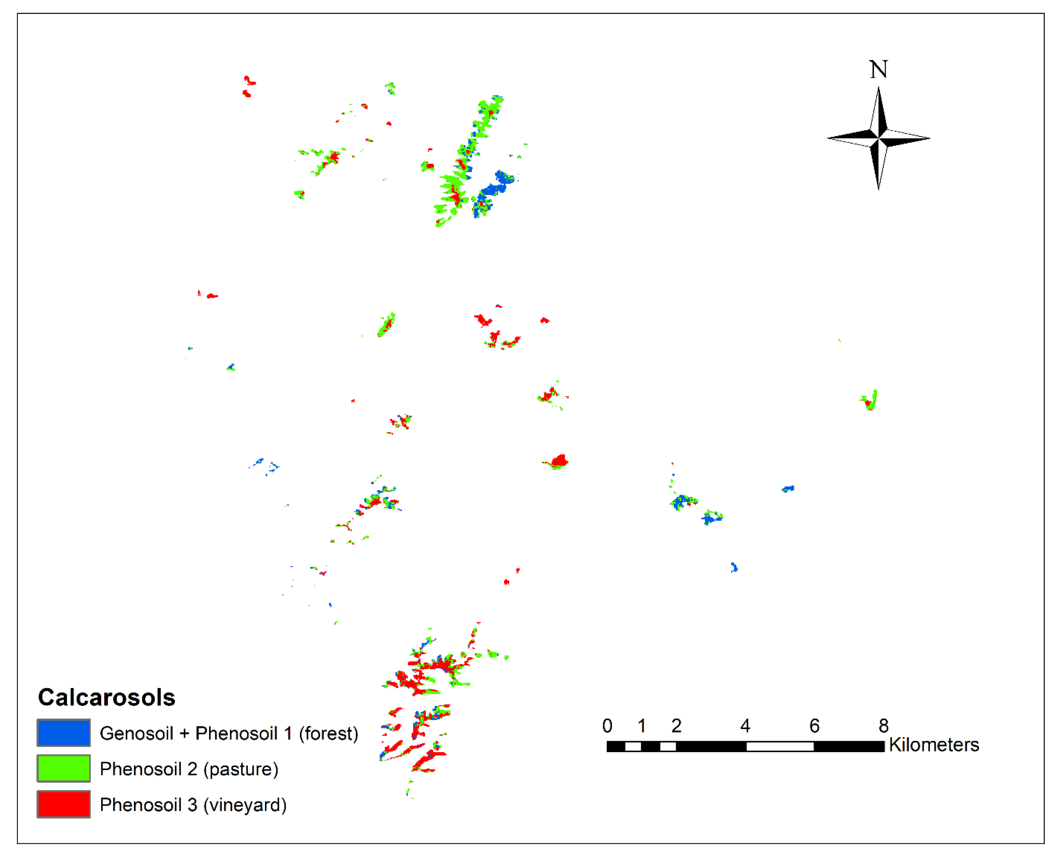
Another example of these analyses includes Calcarosol and the same attributes and depths as the previous example. Here, we compare Calcarosols under forest (combined native forest with sparse forest genosoil 1 and phenosoil 1 in [33]) with Calcarosols in pastures (phenosoil 2) and vineyards phenosoil 3 (Figure 3). In this case, the soil properties of Calcarosols under forest were combined because we had only three soil profile observations under dense forest and seven under sparse forest. All combined forest samples are considered as the reference state. The Calcarosols under pasture, Calcarosol phenosoil 2, are compared [33] with the references state (forest) and other land uses, vineyards.

Phenosoil 2 (pasture) has 37 observations. Using the same soil properties, depths, and order as the Red Chromosol example, the matrices for a Calcarosol forest and pastureland are the following (Table 2);

V = [25.4 37.4 29.4 26.2 45.1 36.4];

Z = [6.2 6.6 5.4 1.8];

U = [25.2 46.3 24.0 25.9 50.8 27.8]; and

Y = [6.8 7.5 4.9 2.0].

Hence,

E = [−0.2 8.9 −5.4 −0.2 5.6 −8.7], with the p-values of [0.99, 0.46 0.52 0.97 0.60 0.44], and

F = [0.7 0.9 −0.5 0.2], with p-values of [0.12, 0.26 0.70 0.88].

For Calcarosols under pasture, the E matrix shows 8% higher clay and equally lower sand contents at 40 to 50 cm deep. If these numbers were significantly different from the reference state, the increased clay indicates that some erosion of the sandy topsoil may have occurred in the pastureland, resulting in the eluvial horizon being closer to the surface in the pasture compared to the reference state. However there are not enough observations to support this conclusion statistically (p-value’s are large).

Second, we compare with Calcarosols under vineyards (Calcarosol phenosoil 3 [33]) to the reference state using an average of 65 observations, Figure 3.), where V and Z are the same.

U = [33.5 50.7 22.0 19.1 44.5 30.2]; and

Y = [6.9 7.7 3.9 2.1].

Hence,

E = [8.1 13.3 −7.4 −7.1 −0.7 −6.2], with p-values of [0.33, 0.18 0.39 0.20 0.94 0.48], and

F = [0.7 1.1 −1.5 0.3], with p-values of [0.07, 0.16 0.12 0.80].

The results of U indicates even more clay in the 40 to 50 cm depth than the reference state and this increase of clay also shows in the topsoil. Soil capacity attributes have changed, but again the number of observations in the reference state hinder a strong statistical interpretation. An alternative interpretation of both E matrices is that there is no remnant vegetation on this soil to compare to; no reference state exists for comparison. This conclusion also might be the case in other longer-developed agricultural regions; we may need to regard the Calcarosol under pasture as the reference state. To continue this point, we can compare the pasture as a reference state with the vineyard area of interest. This kind of comparison is often done by researchers investigating soil quality or soil health, but the analyses are generally focused on the topsoils and only for the attributes that describe the soil condition.

Using the matrices from above, we compare the pasturelands to the vineyards.

E = [8.3 4.4 −2.0 −6.8 −6.3 2.5], with p-values [0.30, 0.63 0.72 0.30 0.43 0.77], and

F = [0.1 0.2 −1.1 0.1], with p-values [0.84 0.59 0.38 0.90].

In these examples, when Calcarosols under vineyard are compared to the same soils in pasture (the average age of vineyards is ~40 years) we still see some increase in clay % (that is still not statistically significant), and potential loss of organic carbon (that is not statistically significant). The change represented in E appears somewhat smaller than when forest is converted to pasture.

4. Discussion and Conclusions

In this short paper, we have presented a generic way of estimating quantities that relate to the actual and potential biophysical ability of soil to perform one or more functions. The approach recognizes that to do assessment of soil change, we need to observe state matrices to describe a soil in its current state and in a reference state. For a given soil, the reference state can be found by using mapped entities described at a particular level in a soil taxonomy and comparing them based on land-use history. Further work is now needed to devise meaningful and estimable ${ℂ}_f$ for each of the soil functions. Kidd et al. [28] suggested a versatile method of estimating ${ℂ}_f$ for the general function biomass production (Function 1, Table 1).

Clearly, we can estimate capability, capacity, and condition of a soil for a range of functions. Should we combine these, and if so, how? A soil could be very multifunctional but is only supplying 50% of its potential relative to the reference state. On the other hand, a soil could only supply a few functions (well) but was doing that at full potential relative to the reference state. There is no doubt in the first case the soil condition can be improved; while in the second, management will not improve the situation. Clearly, in difficult choices of preservation, multifunctional soils may be preferred over unifunctional ones. Soils with highly multifunctional reference states, but which have lost functionality through loss of condition, should be the prime targets for restoration.

We can map either soil functions [37,38] or threats to soil. Instead of trying to map soil functions themselves [38], in soil security we (should) try to evaluate how well a given soil point can perform each function. This recognizes that different soils will have different functionalities even in their pristine condition.

We need to develop an agreement upon the sets of attributes that represent capacity and condition. We need to derive and agree upon appropriate ${ℂ}_f$ for each of the soil functions, and an appropriate level of pedotaxonomic generalisation (soil series or family or higher) for the reference state and a way of spatial delineation of the soil of interest and the reference state. Finally, we need to develop fully worked examples; given that we will have successfully quantified the two biophysical dimensions of soil security in a multifunctional way. This approach presents a worthy and potentially fruitful proposition to soil science and its community of practice.