Statistical and Electrical Features Evaluation for Electrical Appliances Energy Disaggregation

Abstract

In this paper we evaluate several well-known and widely used machine learning algorithms for regression in the energy disaggregation task. Specifically, the Non-Intrusive Load Monitoring approach was considered and the K-Nearest-Neighbours, Support Vector Machines, Deep Neural Networks and Random Forest algorithms were evaluated across five datasets using seven different sets of statistical and electrical features. The experimental results demonstrated the importance of selecting both appropriate features and regression algorithms. Analysis on device level showed that linear devices can be disaggregated using statistical features, while for non-linear devices the use of electrical features significantly improves the disaggregation accuracy, as non-linear appliances have non-sinusoidal current draw and thus cannot be well parametrized only by their active power consumption. The best performance in terms of energy disaggregation accuracy was achieved by the Random Forest regression algorithm.

1. Introduction

With the development of technology and the increasing usage of electrical appliances and automated services, the electric energy needs have been growing steadily for the last century with an annual growth of approximately 3.4% per year in the last decade [1]. Nowadays residential and commercial buildings account already for roughly 36% of the total electrical demand in the USA and 25% in the EU while they are responsible for roughly 43% of carbon dioxide (${\mathrm{CO}}_2$) emissions [2,3,4]. To assure balance between renewable energies, ${\mathrm{CO}}_2$ emissions, political stability and economic growth it is essential to focus on a sustainable development [5]. To achieve sustainable economic growth energy consumption in industrial and residential areas must be minimized under the consideration of rising volatility of nowadays energy production with increasing amounts of renewable energies [6]. Under the consideration of sustainable development several studies investigated real time pricing with additional storage systems [7,8] or large scale energy buffering [6] to reduce electrical energy consumption and peak loads. Other studies indicate that detailed analysis and real-time feedback of energy consumption in residential areas can lead to up to 20% savings in energy consumption through detection of faulty devices and poor operational strategies and thus would improve the sustainability of nowadays consumer households [9,10]. Therefore in the last few decades extensive research in smart grids, smart systems and demand management was carried out and different optimization techniques have been developed to reduce residential energy consumption [11,12,13]. To make use of those techniques, accurate and fine-grained monitoring of electrical energy consumption is needed [14]. However nowadays the energy consumption of most households is monitored via monthly aggregated measurements and therefore cannot provide real-time feedback information.

To measure the energy consumption of a household or building with high resolution in the order of seconds or below smart meters are utilized. According to [15] the largest improvements in terms of energy savings can be made when monitoring energy consumption on device level. Therefore the analysis of energy on device level is performed through energy disaggregation, i.e., the extraction of energy consumption on appliance level based on one or multiple measures from smart meters. When using only one sensor (smart meter) per household or building, therefore measuring only the aggregated consumption, the task is referred to as Non-Intrusive Load Monitoring ($NILM$) [16], in contrast to Intrusive Load Monitoring ($ILM$) where multiple sensors are used, usually one per device. The goal of $NILM$ is to find the inverse of the aggregation function through a disaggregation algorithm using as input only the aggregated power consumption, which makes $NILM$ a highly under-determined problem and thus impossible to solve analytically [17].

In order to solve the $NILM$ problem different approaches have been proposed in literature, which can be split into methods with or without Source Separation ($SS$). Approaches with $SS$ consider the task of energy disaggregation as a single channel source separation problem and extract the corresponding signal of each device from the aggregated samples using a set of conditions and constraints (e.g., sparseness or sum-to-one) [18,19]. Approaches without $SS$ are based on the decomposition of the aggregated signal to a sequence of feature vectors. These feature vectors are then classified to device labels using a machine learning algorithm [8,20,21] or by predefined set of rules or thresholds [22,23]. As machine learning classification/regression models a wide variety of algorithms have been used such as Artificial Neural Networks ($ANNs$) [8], Decision Trees ($DTs$) [24], Hidden Markov Models ($HMMs$) [24,25,26,27,28,29], K-Nearest-Neighbours ($KNNs$) [30], Random Forests ($RFs$) [20], Support Vector Machines ($SVMs$) [24] and ensemble classifiers [31].

Another classification of $NILM$ methods is based on the sampling frequency $f_s$ of the smart meter and thus the features that can be extracted from the measured data [32]. In detail, depending on the sampling frequency either macroscopic (e.g., active/reactive power [23,33,34]) or microscopic (e.g., transient energy, harmonics, wavelets [22,35]) features are extracted to disaggregate energy consumption on appliance level for steady state and transient behaviour, respectively. Macroscopic features are extracted in low sampling frequencies in the order of $\frac{1}{60}$ Hz to 1 Hz while microscopic features are extracted in high sampling frequencies from 50 Hz up to 30 kHz [32]. Many researchers have used microscopic features to efficiently detect transient device behaviour and thus improve energy disaggregation [36,37]. However measuring the power consumption with high sampling frequency has the drawback of higher cost through hardware and increase of computational power [38]. Therefore most studies focus on disaggregation algorithms using macroscopic features or only active power samples in combination with low computational cost disaggregation algorithms utilizing sampling rates in the order of seconds and minutes [28,39,40,41,42,43,44].

Considering the wide range of appliances with either steady-state behaviour [16], where appliances are modelled as finite state machines [16,45] or appliances with transient behaviour including non-linear and continuous appliances [18,36,46], investigation of the effect of different features and classification algorithms is essential. In this paper we evaluate the performance of various well-known and widely used classifiers and various features on the energy disaggregation task for the $NILM$ task. Specifically, we present a large scale evaluation of several features with respect to the $NILM$ performance on specific appliance types in combination with several widely used classification algorithms, in order to investigate which feature sets are more appropriate for accurately detecting specific appliance types, e.g non-linear appliances and the effect of using appliance specific features in the overall $NILM$ performance. The proposed methodology with appliance specific features is evaluated using several combinations of feature sets and classification algorithms.

The remainder of this paper is organized as follows: In Section 2 the baseline $NILM$ system is presented. In Section 3 the experimental setup is described and in Section 4 the evaluation results are presented. Finally conclusions are provided in Section 5.

2. NILM Architecture

$NILM$ energy disaggregation can be formulated as the task of determining the power consumption on device level based on the measurements of one sensor, within time windows (frames or epochs). Specifically, for a set of $M-1$ known devices each consuming power $p_m$ with $1\le m\le M$, the aggregated power $P_{agg}$ measured by the sensor will be

$$P_{agg}=f(p_1,p_2,\dots ,p_{M-1},g)={\displaystyle \sum _{m=1}^{M-1}}{p}_m+g={\displaystyle \sum _{m=1}^M}{p}_m$$

(1)

where $g=p_M$ is a ‘ghost’ power consumption (noise) consumed by one or more unknown devices and f is the aggregation function. In $NILM$ the goal is to find estimations ${\widehat{p}}_m,\widehat{g}$ of the power consumption of each device m using an estimation method $f^{-1}$ with minimal estimation error and ${\widehat{p}}_M=\widehat{g}$, resulting in the total estimated power $\widehat{P}$, i.e.,

$$\begin{array}{c}\widehat{P}=\{{\widehat{p}}_1,{\widehat{p}}_2,\dots ,{\widehat{p}}_{M-1},\widehat{g}\}\leftarrow f^{-1}\left(P_{agg}\right)\\ s.t.\underset{f^{-1}}{argmin}\{{(P_{agg}-{\displaystyle \sum _{m=1}^M}{\widehat{p}}_m)}^2\}\end{array}$$

(2)

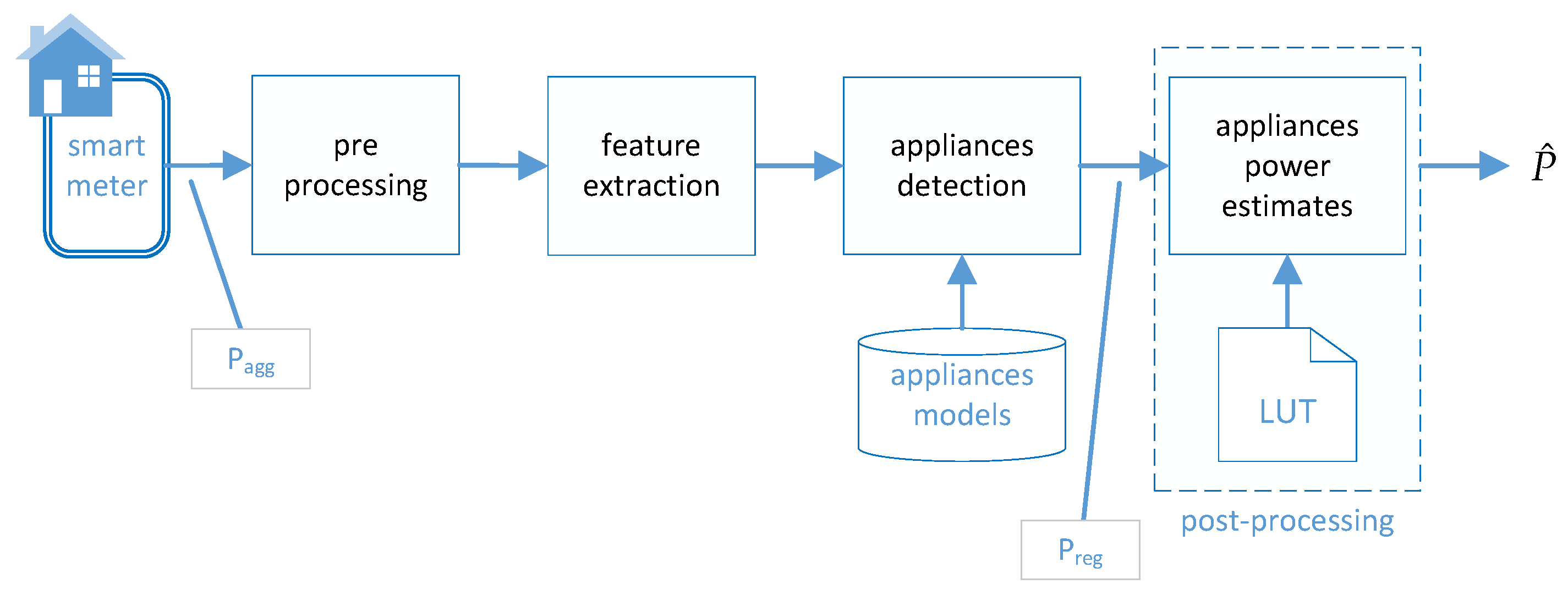
The block diagram of the $NILM$ architecture adopted in the present evaluation is illustrated in Figure 1 and consists of of four stages, namely pre-processing, feature extraction, appliance detection and post-processing. In detail, the aggregated power consumption signal calculated from a smart meter is initially pre-processed, i.e., passed through a median filter [47] and then frame blocked in time frames. After pre-processing feature vectors, v of length $∥v∥$, one for each frame are calculated. In the appliance detection stage the feature vectors are processed by a regression algorithm using a set of pre-trained appliance models to estimate the power consumption of each device. The output of the regression algorithm ($P_{reg}$) estimates the corresponding device consumption and a set of thresholds $T_m$ with $1\le m\le M$ with $T_g=T_M$ for the each device including the ghost device ($m=M$) is used to decide whether a device is switched on or off. The detection of appliances and estimation of their power consumption is performed for each frame of the aggregated signal. A post-processing stage is refining the power estimates form the regression model by mapping them to apriori known device states using a Look-Up-Table ($LUT$), i.e., if the distance of the regression output to any state in the device model is larger than $25W$ the regression output is mapped to the closest device state. In order to define the number of states per device the K-Means algorithm was used for initialisation followed by Expectation-Maximization ($EM$) clustering to calculate the power consumption for each state of each device and form the $LUT$ for the post-processing stage [48].

3. Experimental Setup

The $NILM$ architecture presented in Section 2 was evaluated using a number of publicly available datasets and a number of well-known machine learning algorithms for regression.

3.1. Datasets

To evaluate performance five different datasets of the $ECO$ [47] database were used. The $ECO$ database was chosen as it contains power consumption measurements per device as well as the aggregated consumption. The $ECO$-3 dataset was excluded as it contains only the aggregated signal and not the power consumptions per device. Furthermore the aggregated consumption measurements include not only the active power, but also the line currents ($I_x$), line voltages ($V_x$) and load angles (${\phi }_x$) for all three phases ($x\in \{1,2,3\}$).

The evaluated datasets and their characteristics are tabulated in

Table 1. List of evaluated datasets and their respective properties.

Dataset	Parameters
	#App	${\mathit{T}}_{\mathit{s}}$	T	Appliance Type
ECO-1	7 (6)	1s	7d	One-state/multi-state
ECO-2	12 (9)	1s	7d	One-state/multi-state/non-linear
ECO-4	8 (8)	1s	7d	One-state/multi-state/non-linear
ECO-5	8 (6)	1s	7d	One-state/multi-state/non-linear
ECO-6	7 (6)	1s	7d	One-state/multi-state/non-linear

with the number of appliances denoted in the column $\#App$. In the same column, the number of appliances in brackets is the number of appliances after excluding devices with power consumption below $25W$, which were added to the power of the ghost device, similarly to the experimental setup followed in [40,49]. The next three columns in Table 1 are listing the sampling period $T_s$, the duration T of the aggregated signal used and the appliance type for each evaluated dataset. The appliances type categorization is based on their operation as described in [50,51], i.e., one-state devices have only on/off status (e.g., resistive lamps, kettles or fridges without significant power spikes), multi-state devices having several discrete power consumption states (e.g., washing machines including different washing cycles) and non-linear loads (e.g., electronic appliances) having various states and stronger power variation. Considering their electrical layout all one- and multi-state appliances consist of a series of resistors, inductors and capacitors and thus can further be classified into resistive, inductive and capacitive devices. Non-linear appliances can include additional active components (e.g., semiconductors) and non-linear passive elements (e.g., diodes).

To evaluate $NILM$ performance in close to real conditions the aggregated signal including the ghost power from unknown devices was used as proposed in [52], instead of creating an artificial aggregated signal by adding the corresponding power consumption from each device. The aggregated signal includes real power samples, raw current samples, raw voltage samples and load angles, depending on the chosen feature set.

3.2. Pre-Processing and Feature Ranking

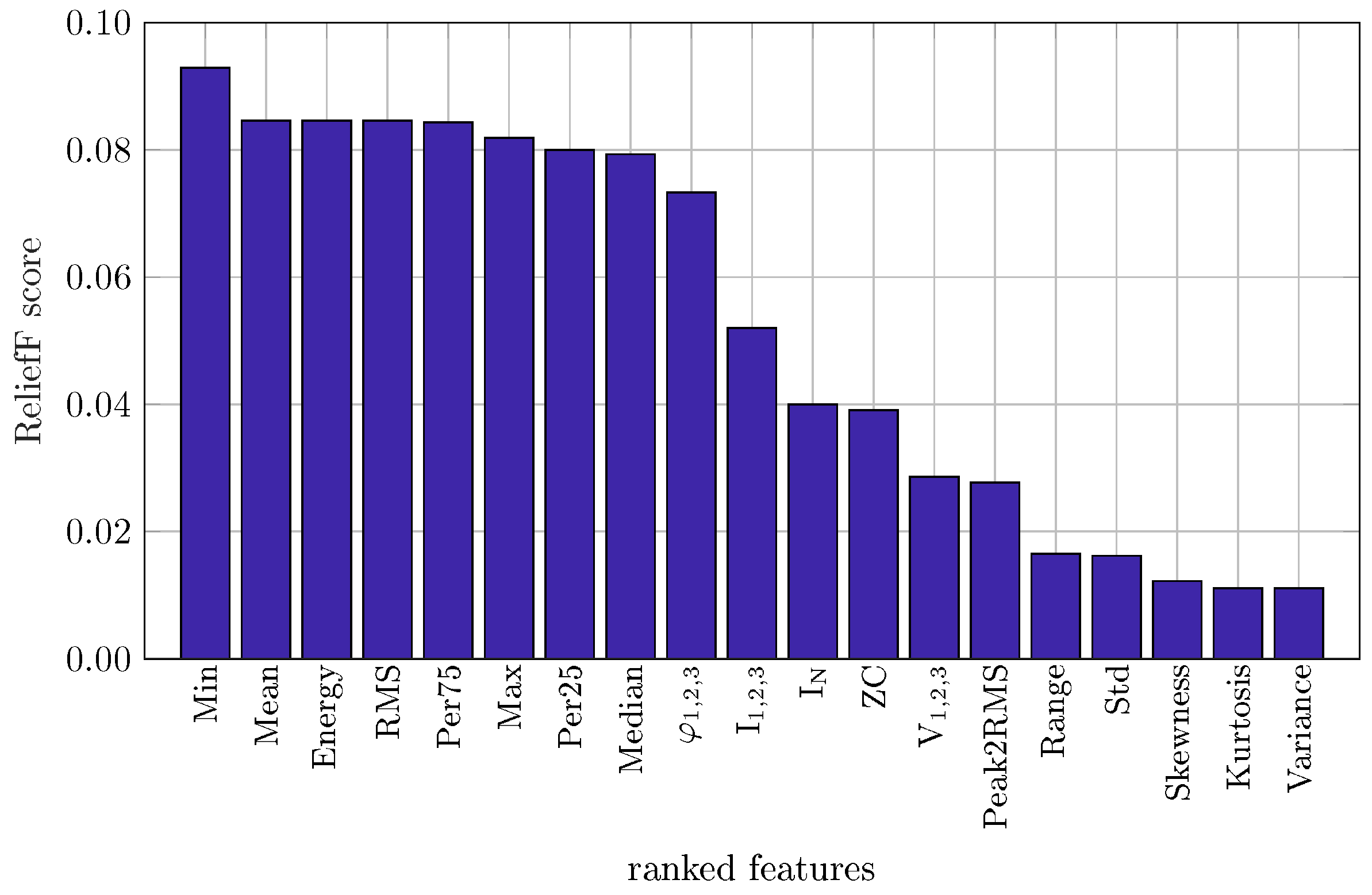
During pre-processing the aggregated signal was processed by a median filter of 5 samples as proposed in [47] and then was frame blocked in frames of 10 samples with overlap between successive frames equal to 50% (i.e., 5 samples). For every frame a feature vector v∈${\mathbb{R}}^D$ consisting of 15 statistical (mean value, minimum and maximum values, Root-Mean-Square ($RMS$) value, median value, percentiles 25% and 75%, variance, standard deviation ($std$), skewness, kurtosis, range, energy and Zero Crossings ($ZC$)) and four electrical features (line current, neutral current, line voltage and load angle) were calculated resulting in a feature vector of dimensionality equal to $D=19$. In order to calculate the statistical importance of the 19 features the $ReliefF$ feature ranking algorithm [53] was used. The $ReliefF$ algorithm was chosen as it can deal with noisy data (in our task mainly coming from the ghost power) and is appropriate for feature ranking estimation of multi-class datasets [54], as the multiple devices of the $NILM$ task. The average $ReliefF$ ranking scores across the five evaluated $ECO$ datasets are shown in Figure 2.

As can be seen in Figure 2 statistical and electrical features can be divided into two groups based on their $ReliefF$ scores. The first group includes eight statistical and three electrical features with high ranking score (≥0.04) namely the Min/Max, Mean, Energy, $RMS$, Percentiles75/25 (Per75/Per25), Median and the load angles (${\phi }_{1,2,3}$), the line currents ($I_{1,2,3}$) and the neutral current ($I_N$), respectively. The second group includes features with lower ranking score (<0.04) namely the Zero Crossing rate, Peak2Rms, Range, Standard Deviation, Skewness, Kurtosis, Variance from the statistical features and the line voltages ($V_{1,2,3}$) from the electrical features. For the electrical features it must be mentioned that the neutral current and the load angles are given by the sum of the line currents and the phase-shift between line currents and voltages, respectively, therefore they carry complementary information which affects their ranking scores.

The outcome of the feature ranking was used to design a set of seven experimental protocols, with the first four including only statistical features and the last three employing the additional electrical features. The chosen features for each experiment are tabulated in

Table 2. Definition of seven different experimental protocols including different numbers of features determined from the feature ranking (experiments 1–4 with statistical features only and experiments 5–7 with additional electrical features).

Protocol	Features	Category
1	Mean	Statistical Features
2	Mean, Max, Min, RMS, Energy	Statistical Features
3	Mean, Max, Min, RMS, Energy, Median, Per25, Per75	Statistical Features
4	Mean, Max, Min, RMS, Energy, Median, Per25, Per75, Peak2Rms, Range, Std, Variance, Skewness, Kurtosis	Statistical Features
5	Statistical Features, Line Currents	Statistical/Electrical Features
6	Statistical Features, Line Currents, Line Voltages	Statistical/Electrical Features
7	Statistical Features, Line Currents, Line Voltages, Load Angles	Statistical/Electrical Features

where the first experiment is only considering the mean value of active power samples and thus is considered as baseline system, while for the following experiments features with decreasing feature score from the feature ranking were added under consideration of keeping similar pairs of features together (e.g., $Min/Max$). There is one exceptional case (in protocol 5/7) for the electrical features were the load angles are added after the line currents/voltages. This is due to two reasons, namely that the combination of line current and voltages contains the same information as the load angles and that load angles can only be computed if line currents and voltages are available.

For the regression stage four different well known and widely used machine learning algorithms have been employed namely the feed-forward Deep Neural Networks ($DNNs$), the k-Nearest Neighbours ($KNNs$), the Random Forests ($RFs$) and the Support Vector Machines ($SVMs$). The free parameters of each regression algorithm were empirically optimized after grid search on a bootstrap training subset including data from the $ECO$-1/2/4/5/6 datasets with ideal aggregated data (without ghost power) as shown in

Table 3. Parametrization results (%) for four different classifiers namely Deep Neural Networks ($DNNs$), Random Forest ($RFs$), K-Nearest-Neighbours ($KNNs$) and Support Vector Machines ($SVMs$).

Deep Neural Network (DNN)
Nodes/ Layers	4	8	16	32	64	128
1	80.42	87.54	87.85	83.73	86.38	81.67
2	70.09	86.39	86.92	87.50	82.68	83.62
3	80.40	86.70	87.86	88.71	88.39	84.20
4	75.40	87.95	87.02	87.15	85.32	x
Random Forest (RF)
Trees	8	16	32	64	128	256
	85.45	85.31	85.47	85.42	85.44	85.42
K-Nearest-Neighbours (KNN)
K	1	2	3	4	5	6
	82.15	82.74	82.68	83.05	83.26	82.42
Support Vector Machine (SVM)
Kernel	Linear	Gaussian	Rbf	Pol-2	Pol-3	Pol-4
	55.02	72.33	76.29	59.24	63.58	67.83

. The best performance corresponding to the optimal values of each regression model is shown in bold. A “one vs. all” approach was chosen with the output of each regression model being the prediction of the power of the $m^{th}$ appliance. In order to avoid overlap between training and test data, each of the evaluated datasets was equally split into two subsets, one for training each regression model and one for evaluating its performance.

As can be seen in Table 3 the parameter optimized regression models are a $DNN$ feed-forward architecture with 3-hidden layers and 32 sigmoid nodes per layer, a $KNN$ with $K=5$ nearest neighbours, a $RF$ with 32 trees per forest and a $SVM$ with Radial Basis Function ($Rbf$) as kernel and optimized kernel parameters $\gamma =12.8$, $C=1.45$. The $DNN$ regression model achieved accuracy equal to 88.71% and outperformed all other evaluated regression models on the bootstrap training set.

4. Experimental Results

The $NILM$ architecture presented in Section 2 was evaluated according to the experimental setup described in Section 3 with the optimized parameters shown in Table 3. The performance was evaluated in terms of power estimation accuracy ($E_{ACC}$), as proposed in [55] and defined in Equation (3). The estimation accuracy is taking into account the estimated power ${\widehat{p}}_m$ and the ground-truth power consumption $p_m$ for each device m, where T is the number of frames and M is the number of disaggregated devices including the ghost power. For evaluating estimation accuracy on device level Equation (3) is modified by eliminating the summation over M appliances resulting in Equation (4) measuring the estimation accuracy on device level ($E_{ACC}^m$).

$$E_{ACC}=1-\frac{{\sum }_{t=1}^T{\sum }_{m=1}^M|{\widehat{p}}_m^t-p_m^t|}{2{\sum }_{t=1}^T{\sum }_{m=1}^M\left|p_m^t\right|}$$

(3)

$$E_{ACC}^m=1-\frac{{\sum }_{t=1}^T|{\widehat{p}}_m^t-p_m^t|}{2{\sum }_{t=1}^T\left|p_m^t\right|}$$

(4)

The evaluation results for different experimental protocols and different regression models are tabulated in

Table 4. Disaggregation results (%) for five different datasets out of the $ECO$ database utilizing four different classifiers ($DNN$, $KNN$, $RF$, $SVM$) with seven experimental protocols each.

ECO-1
Protocol	1	2	3	4	5	6	7
DNN	73.14	70.94	71.94	73.12	77.18	73.52	78.38
KNN	72.56	75.87	75.82	76.02	76.06	75.90	78.92
RF	72.42	77.02	77.00	78.34	79.05	78.23	80.22
SVM	67.04	66.43	66.35	66.84	69.41	67.75	67.98
ECO-2
DNN	83.70	84.69	81.99	85.75	89.78	83.39	89.17
KNN	85.40	85.17	85.22	85.40	85.44	85.26	87.88
RF	83.84	86.16	85.99	86.22	90.03	90.40	91.18
SVM	80.97	71.71	70.85	78.70	81.81	80.64	81.09
ECO-4
DNN	82.42	83.00	81.34	82.45	78.35	84.16	80.78
KNN	80.85	82.16	82.17	82.13	82.50	82.42	83.11
RF	82.27	83.27	83.49	83.84	86.76	86.42	87.49
SVM	77.88	78.79	78.55	80.41	82.35	82.46	81.70
ECO-5
DNN	88.11	86.89	83.48	87.59	91.48	89.47	91.05
KNN	85.63	88.36	88.40	88.08	88.53	88.55	88.88
RF	87.65	88.80	88.83	89.18	93.79	93.78	93.79
SVM	88.62	87.35	86.78	88.42	91.71	91.14	90.18
ECO-6
DNN	80.03	81.30	82.87	82.42	81.94	81.88	68.06
KNN	72.56	75.87	75.82	76.02	76.06	75.90	78.92
RF	79.00	83.39	83.63	84.57	88.32	87.37	80.90
SVM	72.85	70.58	70.23	71.74	72.93	72.77	59.03

. As can be seen in Table 4 adding additional statistical and electrical features improves the energy disaggregation performance across all evaluated datasets, with the $RF$ regression model outperforming all other regression algorithms. In detail for the $RF$ regression model the greatest absolute improvement was observed for the $ECO$-6 dataset (9.32%), followed by the $ECO$-1 dataset (7.80%), while the lowest absolute improvement was found for the $ECO$-3 dataset (5.22%). Moreover, for almost all of the evaluated datasets and regression algorithms the best energy disaggregation performance was achieved when using additional electrical features, i.e., in protocols 5–7.

In order to evaluate the appropriateness of each regression algorithm in the seven experimental protocols the average performance across the five datasets for each of the regression models was calculated. The results are tabulated in

Table 5. Comparison of different regression algorithms for averaged estimation accuracies (% $E_{ACC}$) (average performance across the five datasets $ECO$-1/2/4/5/6) for the seven experimental protocols.

Protocol	1	2	3	4	5	6	7
DNN	81.48	81.36	80.32	82.27	83.75	82.48	81.49
KNN	80.47	83.07	83.16	83.07	83.26	83.17	83.89
RF	81.04	83.73	83.79	84.43	87.59	87.24	86.72
SVM	77.47	74.97	74.55	77.22	79.64	78.95	76.00

.

As can be seen in Table 5, protocol five shows the best average performance for the $DNN$, $SVM$ and $RF$ regression models, while the $KNN$ model shows a slightly higher performance protocol seven followed by protocol five. Moreover, as also shown in Table 4, the $RF$ regression model outperforms the other models (87.6% with 6.5% performance increase), followed by $KNN$ and $DNN$ with similar performance (∼83.8% with 2.5% performance increase), while $SVM$ achieved the lowest performance (79.6% with 1.9% performance increase).

Further analysis of the evaluated results was conducted on appliance type level, as they are described in Section 3 and tabulated in Table 1. The results for per device improvement using the best performing classifier ($RF$) are tabulated in

Table 6. Maximum improvement (%) with respect to the baseline (first) protocol for the best performing regression model ($RF$). The protocol with the best performance is given in brackets. Further devices that are not operating during the testing period are marked in red.

Device	Category	ECO-1	ECO-2	ECO-4	ECO-5	ECO-6
Air-Exhaust	one-state	-	0.00 (1)	-	-	-
Coffee-Maker	one-state	-	-	-	30.97 (5)	0.00 (1)
Dryer	multi-state	24.55 (5)	-	-	-	-
Entertainment	non-linear	-	6.76 (6)	11.12 (6)	18.97 (6)	16.85 (5)
Freezer	one-state	8.87 (7)	2.91 (7)	5.57 (7)	-	-
Fridge	one-state	15.78 (7)	9.76 (7)	22.65 (7)	30.09 (7)	38.16 (5)
Ghost	undefined	3.35 (4)	4.48 (7)	2.46 (5)	3.30 (7)	3.44 (5)
Kettle	one-state	28.42 (6)	-	-	-	14.77 (5)
Kitchen	undefined	-	-	18.59 (4)	-	-
Lamp	one-state	-	0.56 (7)	46.44 (5)	-	-
Laptop	non-linear	-	22.30 (5)	-	2.19 (5)	11.30 (5)
Microwave	multi-state	-	-	23.10 (7)	0.01 (0)	-
Stereo	non-linear	-	8.31 (6)	0.33 (7)	-	-
TV	non-linear	-	5.81 (6)	-	-	-
WM	multi-state	32.24 (4)	-	-	-	-

. The first experimental protocol uses only the mean value of the active power as feature and thus is considered here as baseline system, against which all performance improvements have been calculated in Table 6 with the corresponding protocol denoted in brackets. Moreover appliances that are not operating during the testing are marked in red and were excluded from further investigation.

As can be seen in Table 6 high improvements of performance do not necessarily appear in experimental protocols with the highest number of features. To investigate the relation between appliance types and features on the energy disaggregation task we consider two types of linear appliances, either with pure resistive equivalent circuit diagram or complex loads with inductive/capacitive behaviour. Therefore three appliances categories are formed, namely one/multi-state appliances with resistive behaviour, one/multi-state appliances that can be modelled as complex loads (mainly inductive) and non-linear appliances. This appliance categorization is illustrated in

Table 7. Impact of employing temporal contextual infromation for three different devices categories.

One/Multi-State (Resistive)	One/Multi-State (Inductive)	Non-Linear
$\begin{array}{cc}\hfill P& =V·I\hfill \\ \hfill Q& =0\hfill \end{array}$	$\begin{array}{c}\hfill P=V·I·cos\left(\phi \right)\\ \hfill Q=V·I·sin\left(\phi \right)\end{array}$	$\begin{array}{cc}\hfill P& =\frac{1}{T}{\int }_{t-T}^T{\displaystyle \sum _k^{\infty }}{v}_k·i_{k}dt\hfill \\ \hfill Q& =Q_{reactive}+Q_{non-linear}\hfill \end{array}$
Coffee Maker, Dryer, Kettle, Lamp, Microwave, WM	Fridge, Freezer	Entertainment, Stereo, Laptop, TV

.

After examining the results from Table 6 under the consideration of Table 7 it can be seen that for resistive one/multi-state appliances (e.g., kettle, coffee machine or lamp) where the reactive power is zero ($Q=0$) the best performing experimental protocol is protocol five in which together with the statistical features the line current is included in the feature vector as an electrical feature. For this appliance type adding the line voltage or the load angle as additional feature is not beneficial, since the load angle or the shift between current and voltage is always zero and thus does not contribute to their parametrized power signature with significant information. Except this, one/multi-state appliances with strong inductive behaviour (e.g., fridges or freezers) benefit from adding the load angle as a feature, as they consume a significant amount of reactive power and thus achieved their best performance with experimental protocol seven. In addition, non-linear devices cannot be described in terms of the active and reactive power consumption including the corresponding load angle, since the current flowing through them is non-sinusoidal as illustrated in Table 7. Thus their power consumption must be described through different techniques, as for example the Fryze power theory [56], where time domain analysis of active and non-active currents is used and the reactive power is split into a reactive component caused by the time domain shift between current and voltage and a component caused by the non-linearity of the device. For such appliances (e.g., entertainment, laptop or TV) the best performing experimental protocol was protocol six where line current and line voltage are added as features hence a time domain description is performed as suggested in [56] and does not include the load angle, since in non-linear appliances the load angle does not carry any device-dependent information.

As regards performance on dataset level the maximum overall performance can be achieved when detecting each device using its own set of optimal features (i.e., the best performing experimental protocol) as tabulated in Table 6. Additionally to selecting appliance-driven features the disaggregation results can be improved when employing the post-processing step from Section 2 where the power estimates from the regression stage $P_{reg}$ are mapped to the appliance states determined through the appliance model during the pre-processing. The per dataset results when choosing the optimal set of features individually for each device and utilizing the post-processing are tabulated in

Table 8. Maximum performance (%) per dataset for all classifiers using appliance driven features with (‘Post’) and without post-processing (‘App’) when compared to the best performing protocol without post-procesing and with uniform appliance features for all appliances (‘Base’).

	DNN			KNN			RF			SVM
	Base	App	Post	Base	App	Post	Base	App	Post	Base	App	Post
ECO-1	78.38	81.56	81.86	78.92	79.71	79.32	80.22	81.89	82.47	69.41	69.75	69.85
ECO-2	89.78	90.52	90.61	87.88	90.52	90.47	91.18	91.75	92.39	81.81	83.64	85.25
ECO-4	84.16	85.34	86.56	83.11	83.32	83.34	87.49	87.90	87.99	82.46	84.02	84.88
ECO-5	91.48	92.36	93.13	88.88	89.94	89.62	93.79	93.92	94.54	91.71	92.71	93.21
ECO-6	82.87	83.05	86.62	83.71	84.62	85.24	88.32	89.54	90.13	72.93	75.14	76.58
AVG	85.33	86.57	87.76	84.50	85.62	85.60	88.20	89.00	89.50	79.66	81.05	81.95

with the best performing datasets shown in bold.

As can be seen in Table 8, employing the optimal set of features for each device results in further improvement of the disaggregation accuracy varying from 0.1% to 3.2% depending on the dataset and the regression model. The maximum average performance increase for the best performing classifier ($RF$) is 0.8% with an overall average disaggregation accuracy of 89.0%. When further employing the post-processing as described in Section 2 another performance increase between 0.5% and 1.2% can be observed when utilizing $DNNs$, $RFs$ or $SVMs$. However, no performance increase was observed when using $KNNs$. The performance increase when using $DNNs$, $RFs$ or $SVMs$ is mainly due to one/multi-state linear appliances, which can be modelled as finite-state-machines and benefit from the post-processing step where power estimates are mapped to discrete power states of the corresponding appliance. In terms of absolute improvement $RF$ still outperforms all other classifiers when applying the $LUT$ post-processing with overall disaggregation accuracy equal to 89.5%.

5. Conclusions

In this paper the performance of different classifiers in combination with different sets of features for energy disaggregation in non-intrusive load monitoring was investigated. The evaluation results showed significant importance on the selection of features, with the electrical features being more discriminative than the statistical ones. It was also shown that the optimal choice of features strongly depends on the device type and its electrical characteristics, with the non-linear devices better being disaggregated when using line current and line voltage, while linear devices were disaggregated well with statistical features only. After evaluating energy disaggregation across several datasets, random forest ($RF$) was found the best performing regression algorithm outperforming all other evaluated machine learning algorithms by an absolute performance increase of approximately 6.5%. Moreover, it was shown that, when using device dependent features and device state mapping as post-processing, further improvement in energy disaggregation accuracy can be achieved (up-to 1.3%), resulting in a maximum disaggregation performance of 89.5%. Energy disaggregation and especially non-intrusive load monitoring is a very challenging task. The use of detectors which have been designed, adapted or fine-tuned to the specifications of each appliance is a direction which will result in further improvement of disaggregation performance and, in combination with the recent evolution of deep learning [43,57,58] and the use of big data for training device models, e.g., in the order of years [57], is expected to contribute to even more accurate disaggregation methodologies. Moreover multimodal information other than energy data acquired from smart meters like weather, occupancy or socio-economical events could be supportive for disaggregating the energy consumption of households and buildings [59].

References

- Yu, B.; Tian, Y.; Zhang, J. A dynamic active energy demand management system for evaluating the effect of policy scheme on household energy consumption behavior. Energy 2015, 91, 491–506. [Google Scholar] [CrossRef]
- Elma, O.; Selamogullar, U.S. A survey of a residential load profile for demand side management systems. In Proceedings of the 2017 the 5th IEEE International Conference on Smart Energy Grid Engineering (SEGE), Oshawa, ON, Canada, 14–17 August 2017; Gabbar, H.A., Ed.; IEEE Press: Piscataway, NJ, USA, 2017; pp. 85–89. [Google Scholar] [CrossRef]
- Eurostat. Energy Statistics—An Overview; European Union: Brussels, Belgium, 2018. [Google Scholar]
- Pérez-Lombard, L.; Ortiz, J.; Pout, C. A review on buildings energy consumption information. Energy Build. 2008, 40, 394–398. [Google Scholar] [CrossRef]
- Bilan, Y.; Streimikiene, D.; Vasylieva, T.; Lyulyov, O.; Pimonenko, T.; Pavlyk, A. Linking between Renewable Energy, CO2 Emissions, and Economic Growth: Challenges for Candidates and Potential Candidates for the EU Membership. Sustainability 2019, 11, 1528. [Google Scholar] [CrossRef]
- Sinn, H.W. Buffering volatility: A study on the limits of Germany’s energy revolution. Eur. Econ. Rev. 2017, 99, 130–150. [Google Scholar] [CrossRef]
- Miyazato, Y.; Tahara, H.; Uchida, K.; Celestino Muarapaz, C.; Motin Howlader, A.; Senjyu, T. Multi-Objective Optimization for Smart House Applied Real Time Pricing Systems. Sustainability 2016, 8, 1273. [Google Scholar] [CrossRef]
- Lin, Y.H.; Tsai, M.S. An Advanced Home Energy Management System Facilitated by Nonintrusive Load Monitoring With Automated Multiobjective Power Scheduling. IEEE Trans. Smart Grid 2015, 6, 1839–1851. [Google Scholar] [CrossRef]
- Lee, D.; Cheng, C.C. Energy savings by energy management systems: A review. Renew. Sustain. Energy Rev. 2016, 56, 760–777. [Google Scholar] [CrossRef]
- Zeifman, M.; Roth, K. Viterbi algorithm with sparse transitions (VAST) for nonintrusive load monitoring. In Proceedings of the 2011 IEEE Symposium on Computational Intelligence Applications in Smart Grid, Paris, France, 11–15 April 2011; Staff, I., Ed.; IEEE: Piscataway, NJ, USA, 2011; pp. 1–8. [Google Scholar] [CrossRef]
- Indragandhi, V.; Logesh, R.; Subramaniyaswamy, V.; Vijayakumar, V.; Siarry, P.; Uden, L. Multi-objective optimization and energy management in renewable based AC/DC microgrid. Comput. Electr. Eng. 2018, 70, 179–198. [Google Scholar] [CrossRef]
- Çavdar, İ.; Faryad, V. New Design of a Supervised Energy Disaggregation Model Based on the Deep Neural Network for a Smart Grid. Energies 2019, 12, 1217. [Google Scholar] [CrossRef]
- Gabaldón, A.; Álvarez, C.; Ruiz-Abellón, M.; Guillamón, A.; Valero-Verdú, S.; Molina, R.; García-Garre, A. Integration of Methodologies for the Evaluation of Offer Curves in Energy and Capacity Markets through Energy Efficiency and Demand Response. Sustainability 2018, 10, 483. [Google Scholar] [CrossRef]
- Chis, A.; Rajasekharan, J.; Lunden, J.; Koivunen, V. Demand response for renewable energy integration and load balancing in smart grid communities. In Proceedings of the 2016 24th European Signal Processing Conference (EUSIPCO), Budapest, Hungary, 29 August–2 September 2016; IEEE: Piscataway, NJ, USA, 2016; pp. 1423–1427. [Google Scholar] [CrossRef]
- Meziane, M.N.; Abed-Meraim, K. Modeling and estimation of transient current signals. In Proceedings of the 2015 23rd European Signal Processing Conference (EUSIPCO), Nice, France, 31 August–4 September 2015; pp. 1960–1964. [Google Scholar] [CrossRef]
- Hart, G.W. Nonintrusive appliance load monitoring. Proc. IEEE 1992, 80, 1870–1891. [Google Scholar] [CrossRef]
- Gaur, M.; Majumdar, A. Disaggregating Transform Learning for Non-Intrusive Load Monitoring. IEEE Access 2018, 6, 46256–46265. [Google Scholar] [CrossRef]
- Zhu, Y.; Lu, S. Load profile disaggregation by Blind source separation: A wavelets-assisted independent component analysis approach. In Proceedings of the 2014 IEEE PES General Meeting, National Harbor, MD, USA, 27–31 July 2014; IEEE: Piscataway, NJ, USA, 2014; pp. 1–5. [Google Scholar] [CrossRef]
- Figueiredo, M.; Ribeiro, B.; de Almeida, A. Electrical Signal Source Separation Via Nonnegative Tensor Factorization Using On Site Measurements in a Smart Home. IEEE Trans. Instrum. Meas. 2014, 63, 364–373. [Google Scholar] [CrossRef]
- Bilski, P.; Winiecki, W. Generalized algorithm for the non-intrusive identification of electrical appliances in the household. In Proceedings of the the Crossing Point of Intelligent Data Aquisition & Advanced Computing Systems and East & West Scientists, Bucharest, Romania, 1–23 September 2017; IEEE: Piscataway, NJ, USA, 2017; pp. 730–735. [Google Scholar] [CrossRef]
- Liebgott, F.; Yang, B. Active learning with cross-dataset validation in event-based non-intrusive load monitoring. In Proceedings of the EUSIPCO 2017, Kos, Greece, 28 August–2 September 2017; IEEE: Piscataway, NJ, USA, 2017; pp. 296–300. [Google Scholar] [CrossRef]
- Bilski, P.; Winiecki, W. The rule-based method for the non-intrusive electrical appliances identification. In Proceedings of the IDAACS’2015, Warsaw, Poland, 24–26 September 2015; IEEE: Piscataway, NJ, USA, 2015; pp. 220–225. [Google Scholar] [CrossRef]
- Zhou, Y.; Zhai, Q.; Li, X.; Yang, Y. A method for recognizing electrical appliances based on active load demand in a house/office environment. In Proceedings of the 2017 Chinese Automation Congress (CAC), Jinan, China, 20–22 October 2017; IEEE: Piscataway, NJ, USA, 2017; pp. 3584–3589. [Google Scholar] [CrossRef]
- Basu, K.; Debusschere, V.; Bacha, S.; Maulik, U.; Bondyopadhyay, S. Nonintrusive Load Monitoring: A Temporal Multilabel Classification Approach. IEEE Trans. Ind. Inform. 2015, 11, 262–270. [Google Scholar] [CrossRef]
- Li, Y.; Peng, Z.; Huang, J.; Zhang, Z.; Son, J.H. Energy Disaggregation via Hierarchical Factorial HMM. In Proceedings of the 2nd International Workshop on Non-Intrusive Load Monitoring, Austin, TX, USA, 3 June 2014. [Google Scholar]
- Valera, I.; Ruiz, F.; Svensson, L.; Perez-Cruz, F. Infinite Factorial Dynamical Model. In Proceedings of the NIPS’15 Proceedings of the 28th International Conference on Neural Information Processing Systems-Volume 1, Montreal, QC, Canada, 7–12 December 2015. [Google Scholar]
- Mueller, J.A.; Kimball, J.W. Accurate Energy Use Estimation for Nonintrusive Load Monitoring in Systems of Known Devices. IEEE Trans. Smart Grid 2018, 9, 2797–2808. [Google Scholar] [CrossRef]
- Kong, W.; Dong, Z.Y.; Ma, J.; Hill, D.J.; Zhao, J.; Luo, F. An Extensible Approach for Non-Intrusive Load Disaggregation With Smart Meter Data. IEEE Trans. Smart Grid 2018, 9, 3362–3372. [Google Scholar] [CrossRef]
- Agyeman, K.; Han, S.; Han, S. Real-Time Recognition Non-Intrusive Electrical Appliance Monitoring Algorithm for a Residential Building Energy Management System. Energies 2015, 8, 9029–9048. [Google Scholar] [CrossRef]
- Kim, Y.; Kong, S.; Ko, R.; Joo, S.K. Electrical event identification technique for monitoring home appliance load using load signatures. In Proceedings of the IEEE International Conference on Consumer Electronics (ICCE), Las Vegas, NV, USA, 10–13 January 2014; IEEE: Piscataway, NJ, USA, 2014; pp. 296–297. [Google Scholar] [CrossRef]
- Bilski, P. Non-Intrusive Appliance Load Identification with the Ensemble of Classifiers. In Proceedings of the NILM2016 3rd International Workshop on Non-Intrusive Load Monitoring, Vancouver, BC, Canada, 14–15 May 2016. [Google Scholar]
- Gao, J.; Kara, E.C.; Giri, S.; Berges, M. A feasibility study of automated plug-load identification from high-frequency measurements. In Proceedings of the 2015 IEEE Global Conference on Signal and Information Processing (GlobalSIP), Orlando, FL, USA, 14–16 December 2015; IEEE: Piscataway, NJ, USA, 2015; pp. 220–224. [Google Scholar] [CrossRef]
- Zhao, B.; Stankovic, L.; Stankovic, V. On a Training-Less Solution for Non-Intrusive Appliance Load Monitoring Using Graph Signal Processing. IEEE Access 2016, 4, 1784–1799. [Google Scholar] [CrossRef] [Green Version]
- Bouhouras, A.; Gkaidatzis, P.; Chatzisavvas, K.; Panagiotou, E.; Poulakis, N.; Christoforidis, G. Load Signature Formulation for Non-Intrusive Load Monitoring Based on Current Measurements. Energies 2017, 10, 538. [Google Scholar] [CrossRef]
- Barriquello, C.H.; Borin, V.P.; Campos, A. Approach for home appliance recognition using vector projection length and Stockwell transform. Electron. Lett. 2015, 51, 2035–2037. [Google Scholar] [CrossRef]
- Chang, H.H.; Lian, K.L.; Su, Y.C.; Lee, W.J. Power-Spectrum-Based Wavelet Transform for Nonintrusive Demand Monitoring and Load Identification. IEEE Trans. Ind. Appl. 2014, 50, 2081–2089. [Google Scholar] [CrossRef]
- Chang, H.H. Non-Intrusive Demand Monitoring and Load Identification for Energy Management Systems Based on Transient Feature Analyses. Energies 2012, 5, 4569–4589. [Google Scholar] [CrossRef] [Green Version]
- Koutitas, G.C.; Tassiulas, L. Low Cost Disaggregation of Smart Meter Sensor Data. IEEE Sens. J. 2016, 16, 1665–1673. [Google Scholar] [CrossRef]
- van Cutsem, O.; Lilis, G.; Kayal, M. Automatic multi-state load profile identification with application to energy disaggregation. In Proceedings of the 2017 22nd IEEE International Conference on Emerging Technologies and Factory Automation, Limassol, Cyprus, 12–15 September 2017; IEEE: Piscataway, NJ, USA, 2017; pp. 1–8. [Google Scholar] [CrossRef]
- Wang, H.; Yang, W. An Iterative Load Disaggregation Approach Based on Appliance Consumption Pattern. Appl. Sci. 2018, 8, 542. [Google Scholar] [CrossRef]
- Zhang, C.; Zhong, M.; Wang, Z.; Goddard, N.; Sutton, C. Sequence-to-point learning with neural networks for nonintrusive load monitoring. arXiv 2018, arXiv:1612.09106. [Google Scholar]
- Rehman, A.U.; Lie, T.T.; Valles, B.; Tito, S.R. Low Complexity Event Detection Algorithm for Non- Intrusive Load Monitoring Systems. In Proceedings of the 2018 IEEE Innovative Smart Grid Technologies—Asia (ISGT Asia), Singapore, 22–25 May 2018; IEEE: Piscataway, NJ, USA, 2018; pp. 746–751. [Google Scholar] [CrossRef]
- Le, T.T.H.; Kim, H. Non-Intrusive Load Monitoring Based on Novel Transient Signal in Household Appliances with Low Sampling Rate. Energies 2018, 11, 3409. [Google Scholar] [CrossRef]
- Wang, H.; Yang, W.; Chen, T.; Yang, Q. An Optimal Load Disaggregation Method Based on Power Consumption Pattern for Low Sampling Data. Sustainability 2019, 11, 251. [Google Scholar] [CrossRef]
- Ridi, A.; Hennebert, J. Hidden Markov Models for ILM Appliance Identification. Procedia Comput. Sci. 2014, 32, 1010–1015. [Google Scholar] [CrossRef] [Green Version]
- Zheng, Z.; Chen, H.; Luo, X. A Supervised Event-Based Non-Intrusive Load Monitoring for Non-Linear Appliances. Sustainability 2018, 10, 1001. [Google Scholar] [CrossRef]
- Beckel, C.; Kleiminger, W.; Cicchetti, R.; Staake, T.; Santini, S. The ECO data set and the performance of non-intrusive load monitoring algorithms. In Proceedings of the BuildSys’14, 1st ACM Conference on Embedded Systems for Energy-Efficient Buildings, Memphis, TN, USA, 3–6 November 2014; Srivastava, M., Ed.; ACM: New York, NY, USA, 2014; pp. 80–89. [Google Scholar] [CrossRef]
- Ridi, A.; Gisler, C.; Hennebert, J. Appliance and state recognition using Hidden Markov Models. In Proceedings of the International Conference on Data Science and Advanced Analytics (DSAA), Shanghai, China, 30 October–1 November 2014; Cao, L., Ed.; IEEE: Piscataway, NJ, USA, 2014; pp. 270–276. [Google Scholar] [CrossRef]
- Tabatabaei, S.M.; Dick, S.; Xu, W. Toward Non-Intrusive Load Monitoring via Multi-Label Classification. IEEE Trans. Smart Grid 2017, 8, 26–40. [Google Scholar] [CrossRef]
- Shaw, S.R.; Leeb, S.B.; Norford, L.K.; Cox, R.W. Nonintrusive Load Monitoring and Diagnostics in Power Systems. IEEE Trans. Instrum. Meas. 2008, 57, 1445–1454. [Google Scholar] [CrossRef]
- Zoha, A.; Gluhak, A.; Imran, M.A.; Rajasegarar, S. Non-intrusive load monitoring approaches for disaggregated energy sensing: A survey. Sensors 2012, 12, 16838–16866. [Google Scholar] [CrossRef] [PubMed]
- Pereira, L.; Nunes, N. Performance evaluation in non-intrusive load monitoring: Datasets, metrics, and tools-A review. Wiley Interdiscip. Rev. Data Min. Knowl. Discov. 2018, 8, e1265. [Google Scholar] [CrossRef]
- Urbanowicz, R.J.; Meeker, M.; LaCava, W.; Olson, R.S.; Moore, J.H. Relief-Based Feature Selection: Introduction and Review. J. Biomed. Informat. 2018, 85, 189–203. [Google Scholar] [CrossRef] [PubMed]
- Kononenko, I.; Robnik-Sikonja, M.; Pompe, U. ReliefF for Estimation and Discretization of Attributes in Classification, Regression, and ILP Problems. In Proceedings of the AIMSA-96, Sozopol, Bulgaria, 21–22 September 1996; pp. 31–40. [Google Scholar]
- Kolter, J.Z.; Johnson, M.J. (Eds.) REDD: A Public Data Set for Energy Disaggregation Research. In Proceedings of the SustKDD Workshop on Data Mining Applications in Sustainability, San Diego, CA, USA, 21 August 2011. [Google Scholar]
- Staudt, V. Fryze-Buchholz-Depenbrock: A time-domain power theory. In Proceedings of the 2008 International School on Nonsinusoidal Currents and Compensation, Lagow, Poland, 10–13 June 2008; IEEE: Piscataway, NJ, USA, 2008; pp. 1–12. [Google Scholar] [CrossRef]
- Harell, A.; Makonin, S.; Bajić, I.V. Wavenilm: A Causal Neural Network for Power Disaggregation from the Complex Power Signal. arXiv 2019, arXiv:1902.08736. [Google Scholar]
- Valenti, M.; Bonfigli, R.; Principi, E.; Squartini, S. Exploiting the Reactive Power in Deep Neural Models for Non-Intrusive Load Monitoring. In Proceedings of the 2018 International Joint Conference on Neural Networks (IJCNN), Rio de Janeiro, Brazil, 8–13 July 2018; IEEE: Piscataway, NJ, USA, 2018; pp. 1–8. [Google Scholar]
- Ma, M.; Lin, W.; Zhang, J.; Wang, P.; Zhou, Y.; Liang, X. Towards Energy-Awareness Smart Building: Discover the Fingerprint of Your Electrical Appliances. IEEE Trans. Ind. Inform. 2017, 1. [Google Scholar] [CrossRef]
Figure 1.
Block diagram of the proposed Non-Intrusive Load Monitoring () architecture.
Figure 2.
Feature ranking for 19 different statistical and electrical features determined with the algorithm.