Investment and Management Decisions in Aluminium Melting: A Total Cost of Ownership Model and Practical Applications

Abstract

The well-established Total Cost of Ownership (TCO) concept has been applied to several durable goods industries, including machinery. However, none of the existing TCO models explicitly focus on such highly energy-intensive equipment as metal melting furnaces. In this paper, an application of the TCO concept to aluminium melting furnaces is explored. A TCO model is created and tested through seven case studies in the aluminium die casting industry. Results indicate that the capital expenditure (CAPEX) incurred by the sample companies accounts for only 3–5% of a furnace TCO. Moreover, the melting technology implemented in the furnace highly impacts its TCO, as both the furnace’s thermal efficiency and melting loss (i.e., the fraction of aluminium burnt during the melting process) significantly affect the costs incurred. Moreover, the sample furnaces’ cost effectiveness clearly relies on scale. This evaluation leads to identify technological and managerial levers to reduce a furnace TCO, e.g., by adopting energy-efficient furnaces and by installing centralized, large-sized furnaces to pursue scale economies.

1. Introduction

Aluminium die casting producers incur particularly high costs in the utilization of melting furnaces, especially the cost of energy consumed [1,2]. To reduce the impact of such costs, companies may apply technological levers to improve the efficiency of machinery, equipment and plants, and managerial levers, to enhance the efficiency of business processes, operating procedures and information flows.

Adopting a lifecycle standpoint, the cost effect of such levers can be measured through the computation of the “Total Cost of Ownership” (TCO) of melting furnaces. TCO is defined as the sum of all costs associated with the acquisition, use and maintenance of the referred product or service [3]: thus, TCO computation implies evaluating costs along the lifecycle of the considered object, evaluated with the end user’s viewpoint. Despite being known and used since the late 1920s [4,5,6], the TCO concept was popularized between the 1980s and the 1990s [7], when it was firstly applied to supplier selection [8,9,10].

However, the TCO methodology can also support managers to identify and apply effective technological and managerial levers for cost reduction, and to measure-up their effects. Nonetheless, the few applications of the TCO methodology to the metallurgical industry reported in scientific literature [9,10,11,12,13] do not focus on melting furnaces.

In this paper, a new TCO model of aluminium melting furnaces is developed and then applied to seven small- and-medium-sized producers in the aluminium die casting industry. The paper is structured as follows. Section 2 describes the background and objectives of this research. Section 3 presents the new TCO model of aluminium melting furnaces. Section 4 illustrates the results achieved by applying the new model to seven die casting companies. Such findings are discussed in Section 5. Finally, Section 6 draws some concluding remarks and discusses the limitations of this research.

2. Background

2.1. Aluminium Melting in Die Casting Facilities

Melting is a physical process which results in the complete transition of a substance from solid to liquid. In the metallurgical industry, this process is of central importance to foundries, where melting furnaces are generally used to carry out the melting process, i.e., to liquefy metal ingots and scraps in preparation for a casting process [1]. Among all the techniques to produce semi-finished metal components and product, metal casting is the most ancient and versatile: it consists of pouring molten metal into a mould and then allowing it to solidify again and cool down [14]. The currently utilised die casting process was invented in the late 1830s and has been established since the early twentieth century as a high-rate manufacturing process of non-ferrous components with extremely smooth surfaces and excellent dimensional accuracy [14]. Owing to these characteristics, aluminium die casting accounts for a remarkable worldwide output of 11 million tons of components per year, which equals 59% of the global production of non-ferrous die castings [15].

Since the melting and casting equipment requires large investments, the aluminium die casting process is profitable for large-scale production and high utilization rates. Moreover, it is a high-energy-consuming process, owing to the latent heat that has to be transferred to the metal in order to make it melt. The combination of these characteristics in turn can entail considerable operating costs [14]. The amount of energy and fixed capital required to carry out such process is considerably impacted by the melting furnaces, i.e., the equipment which liquefies metal prior to die casting: empirical studies indicate that the melting department accounts, on average, for 77% of the overall energy consumption of an aluminium die casting facility [16]. Therefore, melting furnaces play a central role in optimising both the net present value and the payback time of investments in aluminium die casting equipment.

The most diffused aluminium melting furnaces include three main types [1,16]:

• Gas crucible furnaces. Aluminium is introduced in a movable or flipping container and is liquefied via heat conduction by an external gas burner. Due to poor thermal efficiency, significant melting loss (i.e., the fraction of aluminium burnt during the melting process) and reduced dimensions, these furnaces are generally used for small-scale production purposes. However, they are characterised by a lower acquisition cost than large-sized furnaces, and provide high flexibility, which makes them suitable for frequent alloy changes.
• Reverberatory furnaces. Aluminium is introduced in a melting chamber and liquefied via heat radiation by a set of burners installed in the chamber’s sidewalls or roof. Thanks to their high production rate, these furnaces are generally suitable for medium- and large-scale production. On the other hand, these furnaces have high acquisition costs and adapting them to low production volumes is difficult.
• Tower furnaces. They are an “optimised” variant of reverberatory furnaces: aluminium is loaded at the top of a vertical pre-heating tower before descending into the melting chamber. The hot gas stream produced by the melting process is conveyed through the pre-heating tower and heats the solid aluminium before it enters the melting chamber. Thus, tower furnaces have a higher thermal efficiency and a lower melting loss as compared to the reverberatory furnaces, though being affected by the same limitations.

Table 1 summarises the technological features of the melting furnaces described above.

Table 1. Technological Features of Aluminium Melting Furnaces [1,16].

Furnace Type	Thermal Efficiency (% of Input Energy)	Melting Loss (% of Input Aluminium)	Advantages	Limitations
Crucible (gas-fired)	7–19%	3–4%	Low acquisition cost Limited floor occupation High flexibility	Low production rate Poor thermal efficiency High melting loss
Reverberatory	32–40%	2–5%	High production rate Low maintenance costs Large buffer capacity	Large floor space requirements Energy dispersion through exhaust gases High melting loss
Tower	40–48%	1–2%	High production rate Large buffer capacity Optimised energy dispersion and floor space requirements Low melting loss	Height occupation High maintenance costs

2.2. The Total Cost of Ownership (TCO) Concept

The TCO concept implies the adoption of a value-chain [11,17] and lifecycle-oriented approach [3,12] Therefore, TCO is informally defined as the “true cost” of buying a product or service from a supplier [8,10,18].

Although a clear, standardized procedure to compute the TCO of a given good is not defined [19,20], TCO models in the literature have several features in common, including:

• There is the need to consider costs arising before, during and after the procurement process, respectively [3,21]. Post-transaction costs, in turn, include costs related to the good’s utilization, maintenance and disposal [12,17,22].
• They adopt Activity-Based Costing [10,23] and/or Life Cycle Costing [24,25] procedures to allocate the costs of relevant resources to the studied good.
• They focus on monetary costs incurred by the good’s user or owner [10,25,26].

The TCO concept was popularized in 1987 by Gartner Consulting Group, as a methodology to assess the actual cost of investments in corporate computing systems [7]. Since then, researchers and practitioners have established TCO as a valid methodology to support both supplier selection processes [3,12] and utilization of products or services [17] decisions. In the last 15 years, the TCO concept has been extensively applied to heterogeneous industries, predominantly Information Technology (IT) [27,28,29,30], telecoms [31,32,33] and automotive [26,34,35].

2.3. Application of the TCO Methodology to the Machinery Industry

Several TCO models have been proposed for heterogeneous kinds of machinery. The production equipment addressed includes assembly lines and networks [36,37,38], production lines [13,39] and production machines [19,40,41]. Other authors focus on heavy equipment, such as construction and mining machines [42] and forklifts [43]. Few studies address the application of the TCO methodology to fluid machinery, such as hydraulic pumps [44] and heat pumps [45].

Table 2 provides an overview of existing applications of the TCO concepts to the machinery industry, comparing the standpoints, the indicators measured and the decisions supported. TCO models of machines aim to support different decisions over a machine lifetime, such as:

Table 2. Applications of the TCO Methodology to the Machinery Industry.

ID	References	Target(s)	Proposed model
			Model object	Point of view	Supported decision(s)	Explicit formulae?	Indicator(s)
1	[19]	Comparing the total costs of a tinting machine incurred by machine manufacturers, paint producers and paint retailers	Tinting machines	Supply-chain	Machine utilisation	No	TCO
2	[42]	Proposing and testing a lifecycle cost model of heavy equipment for the mining industry	Heavy equipment	Industrial customer/user	Machine utilisation	Yes	Lifecycle Cost (LCC), TCO
3	[37]	Comparing the lifecycle costs and performances of manual and semi-automated assembly lines for the manufacturing industry	Assembly lines	Industrial customer/user	Design, configuration	Yes	Cost of Ownership (COO), Overall Equipment Effectiveness (OEE)
4	[13]	Identifying the configuration and utilisation strategies which minimise the total cost and the environmental impact of a car body welding line	Welding lines	Industrial customer/user	Machine utilisation	No	TCO, Environmental Impact [tons CO2 eq.]
5	[39]	Identifying the configuration and utilisation strategies which minimise the total cost and the environmental impact of a cast-iron components finishing line	Finishing lines	Industrial customer/user	Machine utilisation	No	TCO, Environmental Impact [tons CO2 eq.]
6	[48]	Comparing the overall costs of retrofitting standard electric engines vs. replacing them with high-efficiency engines	Electric engines	Industrial customer/user	Replacement, substitution	Yes	Lifecycle Savings (LCS), Payback Time
7	[49]	Analysing the impact of different obsolescence mitigation strategies on the total cost of machines or complex systems	Spare parts	Industrial customer/user	Replacement, substitution	Yes	TCO, Expected Reward
8	[45]	Comparing the total costs of air/water heat pumps adopting variable speed control vs. “on–off” control	Heat pumps	Private customer/user	Machine utilisation	Yes	TCO, Savings
9	[38]	Identifying the machines and buffers configuration which maximise the production rate of an assembly network, subject to a total cost constraint	Assembly networks	Industrial customer/user	Design, configuration	Yes	TCO, Production Rate
10	[44]	Determining the total cost of hydraulic pumps	Machine	Industrial customer/user	Supplier and product selection	Yes	Total Cost (TC)
11	[36]	Determining the total cost of automated assembly lines for the manufacturing of optoelectronic equipment	Assembly line	Industrial customer/user	Design, configuration	Yes	Cost of Ownership (COO)
12	[47]	Identifying the least-cost supplier selection strategy for non-repairable components of machines or complex systems	Spare parts	Industrial customer/user	Supplier and product selection	Yes	TCO
13	[43]	Comparing the total costs of hydrogen-feed, “fast charge” and electric forklifts	Forklifts	Industrial customer/user	Supplier and product selection	No	TCO, Net Present Cost (NPC)
14	[46]	Selecting the least-cost procurement strategy for spare electric engines, subject to random failure frequency and repair time	Engines	Industrial customer/user	Supplier and product selection	Yes	Cost of Ownership (COO)
15	[41]	Computing the total cost of injection moulding machines, considering both deterministic and stochastic elements (e.g., energy demand over time, frequency and duration of emergency maintenance works)	Injection moulding machines	Industrial customer/user	Supplier and product selection	No	TCO
16	[40]	Comparing the costs of alternative nanoimprinting technologies for the semiconductor industry	Machine	Industrial customer/user	Design, configuration	No	Cost of Ownership (COO)

• design or configuration [36,37,40];
• supplier and product selection [43,44,46,47]; and
• machine utilisation optimisation [13,19,39,45].

In particular, whereas several authors use the TCO methodology to merely compare the cost effectiveness of alternative equipment [43,45,48], others have addressed the effects of machine productivity [36,37,40,46], failure rate or expected duration of critical components [47,49] or end user’s operational modalities [13,39,41] on the TCO of a machine.

Thus, authors have already explored the adoption of output-dependent TCO indicators [36,40,46] and the integration between the TCO and the Overall Equipment Effectiveness (OEE) [37] or the environmental impact of the machine [13,39].

Moreover, the TCO concept’s application to the metallurgical industry has already been explored [9,10,11,12,39]; however, none of their TCO models focus on melting furnaces. On the other hand, the existing TCO methodology applications in the machinery industry (see Section 2.3) provide helpful suggestions for structuring our model.

2.4. Research Setting

This research addresses two major questions:

(1)

How can the TCO of melting furnaces be modelled?

(2)

Can the TCO methodology help to identify relevant cost reduction levers for melting furnaces?

To this purpose, this research aimed:

• to develop and test a TCO model specifically designed for aluminium melting furnaces;
• to identify the main determinants of aluminium melting furnaces’ TCO; and
• to identify cost reduction levers applicable to aluminium die casting producers.

3. The TCO Model for Aluminium Melting Furnaces

The new TCO model of aluminium melting furnaces aims to evaluate all relevant costs associated with the acquisition, utilization, maintenance and disposal of a furnace, adopting the viewpoint of an aluminium die casting producer, i.e., the furnace user. Moreover, it focuses on the processes required to transform aluminium ingots and scraps into molten aluminium at an optimal temperature for the subsequent casting process. Furnace loading and unloading processes are also considered in the model.

On the contrary, such processes taking place in the die casting facility but not directly pertaining to the furnaces, such as mould making, casting and finishing; stock control and inventory planning, or inbound and outbound logistics, are not considered by the model.

As suggested by several researchers [9,20,21,50,51], an Activity-Based Costing (ABC) procedure is adopted to allocate the costs of resources required to operate and supervise the furnace within the activities carried out at any stage of its lifecycle. To this purpose, costs are divided in:

• Capital expenditures (CAPEX), which companies incur to acquire the furnace and related tools and machinery, include:

  ○

  the costs of purchasing the furnace itself ($T{C}_F$); and

  ○

  tooling and equipment ($T{C}_M$): other equipment used to support the melting process (e.g., automatic loading and unloading systems).

• Operating expenditures (OPEX), which companies incur to run the furnace and carry out the production of molten aluminium, include:

  ○

  energy ($T{C}_E$): costs of the sources consumed by the furnace (e.g., natural gas, electricity);

  ○

  labour ($T{C}_L$): costs of the personnel assigned to furnace operation and supervision (e.g., direct operators, maintenance staff, etc.); and

  ○

  materials ($T{C}_M$): costs of direct and indirect goods consumed by the furnace (e.g., aluminium wasted due to melting loss of the furnace, de-slagging salt, etc.).

Accordingly, the overall TCO of a melting furnace is the sum of all costs listed above:

$$\overline{TCO}=CAPEX+OPEX=\left(T{C}_F+T{C}_M\right)+\left(T{C}_E+T{C}_L+T{C}_M\right)$$

(1)

By dividing the overall TCO of a melting furnace by its projected lifecycle output, a TCO per output unit or unit TCO indicator can also be computed:

$$TCO=\frac{1}{{{\displaystyle \sum }}_t{{\displaystyle \sum }}_a\left\{T{P}_a\left(t\right)\right\}}·\overline{TCO}$$

(2)

The following paragraphs describe the computation procedures adopted for the five cost categories included in Equation (1).

3.1. Total Cost of the Furnace

The total cost of the furnace ($T{C}_F$) can be computed as the difference between the initial purchase price of the furnace ($p_F$) and its discounted residual value ($r{v}_F$), if any:

$$T{C}_F=p_F-\left[r{v}_F·\frac{1}{{\left(1+r\right)}^{LC}}\right]$$

(3)

3.2. Total Cost of Tooling and Equipment

The total cost of tooling and equipment ($T{C}_T$) can be computed by summing, for every tool or piece of equipment j, the difference between its initial purchase price ($p_j$) and its discounted residual value ($r{v}_j$), if any.

$$T{C}_T={\displaystyle \sum }_j\left\{p_j-\left[r{v}_j·\frac{1}{{\left(1+r\right)}^{LC}}\right]\right\}$$

(4)

3.3. Total Cost of Energy

Generally, four operating statuses can be identified over the lifecycle of aluminium melting furnaces:

Inactivity: The furnace is emptied out and turned off due to either scheduled stops (e.g., plant closing and scheduled maintenance) or unscheduled stops (e.g., relevant furnace failure or malfunctioning). The amount of energy consumed during this status is negligible.

Switch-on: The furnace is reactivated after a (scheduled or unscheduled) stop. The furnace temperature must be gradually increased, otherwise the inner refractory shell would be damaged by thermal shock. Consequently, a temporary, yet steady increase of power is required to reactivate the furnace.

Melting: The furnace is loaded with metal charge, but the aluminium is not completely liquefied yet. Consequently, the energy consumed by the furnace is destined to the melting process, regardless of the availability of downstream machines (e.g., die casting machines).

Holding: The metal charge is completely liquefied, but the downstream machines are not ready to process it. Accordingly, the furnace consumes energy to keep the molten aluminium at optimal temperature for the die casting process until the downstream machines become available to process it.

Since the amount of energy consumed by a melting furnace varies significantly considering different operating statuses, the costs related to energy consumption during the melting status ($C_{E,melt}\left(t\right))$, the holding status ($C_{E,hold}\left(t\right)$) and the switch-on status ($C_{E,swit}\left(t\right)$) are computed separately. The total cost of energy ($T{C}_E$) is then obtained by discounting and summing these costs:

$$T{C}_E={\displaystyle \sum }_t\left\{\left[C_{E,melt}\left(t\right)+C_{E,swit}\left(t\right)+C_{E,hold}\left(t\right)\right]·\frac{1}{{\left(1+r\right)}^t}\right\}$$

(5)

The following sections explain the procedure to compute the duration and the energy cost of each operating status.

3.3.1. Inactivity Status

As mentioned above, the amount of energy consumed by a furnace during the inactivity status is negligible. However, computing the duration of this status ($D_{off}\left(t\right)$) is still required to estimate the total cost of energy: to this purpose, the durations of plant closings ($D_{clos}\left(t\right)$), of furnace setups ($D_{setup}\left(t\right)$) and of both routine and emergency maintenance works ($D_{rman}\left(t\right)$ and $D_{eman}\left(t\right)$, respectively) must be summed up.

$$D_{off}\left(t\right)=D_{clos}\left(t\right)+D_{setup}\left(t\right)+D_{rman}\left(t\right)+D_{eman}\left(t\right)$$

(6)

The overall duration of plant closings ($D_{clos}\left(t\right)$) is computed by summing the duration of holiday, weekly and daily closings. In particular:

• The yearly duration of holiday closings is equal to $x_{holi}\left(t\right)·\left[52-N_{weeks}\left(t\right)\right]·7·24$ [hours/year].
• the yearly duration of weekly closings is equal to $x_{weeks}\left(t\right)·N_{weeks}\left(t\right)·\left[7-N_{days}\left(t\right)\right]·24$ [hours/year].
• the yearly duration of daily closings is equal to $x_{days}\left(t\right)·N_{weeks}\left(t\right)·N_{days}\left(t\right)·\left[24-N_{hours}\left(t\right)\right]$ [hours/year].

Combining all terms above results in:

$$\begin{gathered} D_{clos}\left(t\right)=x_{holi}\left(t\right)·\left[52-N_{weeks}\left(t\right)\right]·7·24+N_{weeks}\left(t\right)·\left\{x_{weeks}\left(t\right)·\left[7-N_{days}\left(t\right)\right]· \\ 24+x_{days}\left(t\right)·N_{days}\left(t\right)·\left[24-N_{hours}\left(t\right)\right]\right\} \end{gathered}$$

(7)

The overall duration of stops due to furnace setups ($D_{setup}\left(t\right)$) is obtained by multiplying the number of stops due to setup ($S_{setup}\left(t\right)$) and their unitary duration ($d_{setup}$):

$$D_{setup}\left(t\right)=S_{setup}\left(t\right)·d_{setup}$$

(8)

The number of stops due to setup, in turn, equals the overall number of setups ($N_{setup}\left(t\right)$) multiplied by the furnace status during setups ($x_{setup}\left(t\right)$):

$$S_{setup}\left(t\right)=x_{setup}\left(t\right)·N_{setup}\left(t\right)$$

(9)

Considering that routine maintenance works generally overlap, the number of stops due to routine maintenance ($D_{rman}\left(t\right)$) is approximated by multiplying the average frequency ($f{r}_w\left(t\right)$) by the duration ($d_w$) and the furnace status ($x_w\left(t\right)$) for each routine maintenance work w, and by considering the maximum among the resulting values:

$$\begin{array}{cc}{D}_{rman}\left(t\right)=\max \left\{f{r}_w\left(t\right)·d_w·x_w\left(t\right)\right\}& \forall w\end{array}$$

(10)

As emergency maintenance works occur randomly and independently of each other, the number of stops due to emergency maintenance ($D_{eman}\left(t\right)$) can be computed by summing up the products among the expected frequency ($f{e}_w\left(t\right)$), the duration ($d_w$) and the furnace status ($x_w\left(t\right)$) for any emergency maintenance work w:

$$D_{eman}\left(t\right)={{\displaystyle \sum }}_w\left\{f{e}_w\left(t\right)·d_w·x_w\left(t\right)\right\}$$

(11)

3.3.2. Switch-On Status

Generally, the energy consumption during the switch-on status is time-dependent, i.e., it is expressed in energy per unit of time. Accordingly, the related cost ($C_{E,swit}\left(t\right)$) is computed as the overall duration of the switch-on status ($D_{swit}\left(t\right)$), multiplied by the corresponding energy consumption ($k_{E,hold}\left(t\right)$) and the unitary cost of energy ($c_E\left(t\right)$):

$$C_{E,swit}\left(t\right)=D_{swit}\left(t\right)·k_{E,swit}\left(t\right)·c_E\left(t\right).$$

(12)

The overall duration of the switch-on status ($D_{swit}\left(t\right)$) is equal to the average duration of a single switch-on event ($d_{swit}$), multiplied by the total number of stops related to plant closings, setups, routine and emergency maintenance works ($S_{clos}\left(t\right)$, $S_{setup}\left(t\right)$, $S_{rman}\left(t\right)$ and $S_{eman}\left(t\right)$, respectively), since each stop is followed by a switch-on:

$$D_{swit}\left(t\right)=d_{swit}·\left[S_{clos}\left(t\right)+S_{setup}\left(t\right)+S_{rman}\left(t\right)+S_{eman}\left(t\right)\right]$$

(13)

The actual number of stops due to plant closings ($S_{clos}\left(t\right)$) is deduced from the number of holidays ($N_{holi}\left(t\right)$), of working weeks per year ($N_{weeks}\left(t\right)$) and of working days per week ($N_{days}\left(t\right)$), considering the furnace status during holiday, weekly and daily closings ($x_{holi}\left(t\right)$, $x_{weeks}\left(t\right)$ and $x_{days}\left(t\right)$, respectively):

$$S_{clos}\left(t\right)=x_{holi}\left(t\right)·N_{holi}\left(t\right)+N_{weeks}\left(t\right)·\left[x_{weeks}\left(t\right)+x_{days}\left(t\right)·N_{days}\left(t\right)\right]$$

(14)

Considering that routine maintenance works generally overlap, the number of stops due to routine maintenance ($S_{rman}\left(t\right)$) is approximated by the maximum frequency ($f{r}_w\left(t\right)$) among those routine maintenance works, which require turning off the furnace ($x_w\left(t\right)=1$):

$$\begin{array}{cc}{S}_{rman}\left(t\right)=\max \left\{x_w\left(t\right)·f{r}_w\left(t\right)\right\}& \forall w\end{array}$$

(15)

As emergency maintenance works occur randomly and independently of each other, the number of stops due to emergency maintenance ($S_{eman}\left(t\right)$) can be computed by summing the frequencies ($f{e}_w\left(t\right)$) of all the emergency maintenance works which require turning off the furnace ($x_w\left(t\right)=1$):

$$S_{eman}\left(t\right)={{\displaystyle \sum }}_w\left\{x_w\left(t\right)·f{e}_w\left(t\right)\right\}$$

(16)

3.3.3. Melting Status

Typically, the energy consumption during the melting status is input-dependent, i.e., it is expressed in energy per unit of processed material. For any alloy a processed by the furnace, the overall input ($I{N}_a\left(t\right)$) is deduced from the corresponding output ($T{P}_a\left(t\right)$) considering any loss effect of the melting process ($l\left(t\right)$):

$$I{N}_a\left(t\right)=\frac{1}{1-l\left(t\right)}·T{P}_a\left(t\right)$$

(17)

The cost of the energy consumed during the melting status ($C_{E,melt}\left(t\right)$) is obtained by multiplying the overall input to the furnace (${\displaystyle \sum }_a\left\{I{N}_a\left(t\right)\right\}$) by the unitary energy consumption of the furnace in this status ($k_{E,melt}\left(t\right)$) and the unitary cost of energy ($c_E\left(t\right)$):

$$C_{E,melt}\left(t\right)={\displaystyle \sum }_a\left\{I{N}_a\left(t\right)\right\}·k_{E,melt}\left(t\right)·c_E\left(t\right)$$

(18)

Although this cost is independent of the duration of the melting status ($D_{melt}\left(t\right)$), computing this time quantity is still required to estimate the total cost of the energy consumed by the furnace: to this purpose, the overall input (${\displaystyle \sum }_a\left\{I{N}_a\left(t\right)\right\}$) must be divided by the actual production rate of the furnace ($p{c}_{ac}\left(t\right))$.

$$D_{melt}\left(t\right)=\frac{{{\displaystyle \sum }}_a\left\{I{N}_a\left(t\right)\right\}}{p{c}_{ac}\left(t\right)}$$

(19)

The actual production rate of the furnace ($p{c}_{ac}\left(t\right)$) is obtained by multiplying the standard production rate ($p{c}_{st}$) by the velocity yield of the furnace ($pr\left(t\right)$):

$$p{c}_{ac}\left(t\right)=p{c}_{st}·pr\left(t\right)$$

(20)

3.3.4. Holding Status

Generally, the energy consumption during the holding status is time-dependent: accordingly, the related cost ($C_{E,hold}\left(t\right)$) is obtained as the product among the overall duration of this status ($D_{hold}\left(t\right)$), the unitary energy consumption of the furnace ($k_{E,hold}\left(t\right)$) and the unitary cost of energy ($c_E\left(t\right)$):

$$C_{E,hold}\left(t\right)=D_{hold}\left(t\right)·k_{E,hold}\left(t\right)·c_E\left(t\right)$$

(21)

The overall duration of the holding status can be measured empirically through any furnace monitoring system. Alternatively, it can be deduced by computing the difference between the duration of a solar year, i.e., 8760 [hours/year], and the overall durations of the inactivity, switch-on and melting statuses ($D_{off}\left(t\right)$, $D_{swit}\left(t\right)$ and $D_{melt}\left(t\right)$, respectively):

$$D_{hold}\left(t\right)=8760-\left[D_{swit}\left(t\right)+D_{off}\left(t\right)+D_{melt}\left(t\right)\right]$$

(22)

3.4. Total Labour Cost

The total labour cost ($T{C}_L$) can be computed by summing the discounted costs of the personnel assigned to furnace operation and supervision ($C_{L,fond}\left(t\right)$) and to furnace maintenance ($C_{L,mant}\left(t\right)$):

$$T{C}_L={\displaystyle \sum }_t\left\{\left[C_{L,fond}\left(t\right)+C_{L,mant}\left(t\right)\right]·\frac{1}{{\left(1+r\right)}^t}\right\}$$

(23)

The cost of the personnel assigned to furnace operation and supervision ($C_{L,fond}\left(t\right)$) is computed by summing the products between the number of full-time equivalents ($FT{E}_e\left(t\right)$) and the unitary cost of labour ($c_{L,e}\left(t\right)$) for each category of employees e; the resulting “weighted” cost is then multiplied by the number of daily work shifts ($N_{shift}\left(t\right)$):

$$C_{L,fond}\left(t\right)=N_{shift}\left(t\right)·{{\displaystyle \sum }}_e\left\{FT{E}_e\left(t\right)·c_{L,e}\left(t\right)\right\}$$

(24)

Likewise, the cost of the personnel assigned to furnace maintenance ($C_{L,mant}\left(t\right)$) is computed by summing the products among the unitary cost of labour ($c_{L,mant}\left(t\right)$), the duration ($d_w$) and the overall frequency of each maintenance work w (given by the sum of its frequency in routine and in emergency modes, $f{r}_w\left(t\right)$ and $f{e}_w\left(t\right)$, respectively):

$$C_{L,mant}\left(t\right)={{\displaystyle \sum }}_w\left\{c_{L,mant}\left(t\right)·d_w·\left[f{r}_w\left(t\right)+f{e}_w\left(t\right)\right]\right\}$$

(25)

3.5. Total Cost of Materials

The total cost of materials ($T{C}_M$) can be computed by summing the discounted costs of lost aluminium ($C_{M,loss}\left(t\right)$), of wearing parts and consumables ($C_{M,fond}\left(t\right)$) and of materials consumed during furnace maintenance ($C_{M,mant}\left(t\right)$):

$$T{C}_M={\displaystyle \sum }_t\left\{\left[C_{M,loss}\left(t\right)+C_{M,fond}\left(t\right)+C_{M,mant}\left(t\right)\right]·\frac{1}{{\left(1+r\right)}^t}\right\}$$

(26)

The overall cost of lost aluminium ($C_{M,loss}\left(t\right)$) is obtained by summing, for every alloy a, the quantity wasted during the melting process (equal to the difference between the overall input, $I{N}_a\left(t\right)$, and the projected output, $T{P}_a\left(t\right)$) and the average unitary cost of material (${\overline{c}}_a\left(t\right)$):

$$C_{M,loss}\left(t\right)={{\displaystyle \sum }}_a\left\{\left[I{N}_a\left(t\right)-T{P}_a\left(t\right)\right]·{\overline{c}}_a\left(t\right)\right\}$$

(27)

The average unitary cost of aluminium alloy a (${\overline{c}}_a\left(t\right)$) is deduced from the unitary cost of ingots ($c_a\left(t\right)$) and the average percentage of scraps in the metal charge ($s_a\left(t\right)$), under the assumption that the die casting company incurs no cost for re-processing internal scraps:

$${\overline{c}}_a\left(t\right)=\left[1-s_a\left(t\right)\right]·c_a\left(t\right)$$

(28)

The overall cost of the materials consumed during furnace operation ($C_{M,fond}\left(t\right)$), such as de-slagging salts, is obtained by summing the products between the input quantity ($Q_m\left(t\right)$) and the unitary cost ($c_m\left(t\right)$), for every material m:

$$C_{M,fond}\left(t\right)={{\displaystyle \sum }}_m\left\{Q_m\left(t\right)·c_m\left(t\right)\right\}$$

(29)

At last, the overall cost of the materials consumed during furnace maintenance ($C_{M,mant}\left(t\right)$) is computed summing the products among the unitary cost of material m ($c_m\left(t\right)$), the quantity of material m consumed during maintenance work w ($q_{m,w}$) and the overall frequency of maintenance work w (given by the sum of its frequency in routine and in emergency modes, $f{r}_w\left(t\right)$ and $f{e}_w\left(t\right)$, respectively), for every combination of materials m and maintenance works w:

$$C_{M,mant}\left(t\right)={\displaystyle \sum }_m{\displaystyle \sum }_w\left\{c_m\left(t\right)·q_{m,w}·\left[f{r}_w\left(t\right)+f{e}_w\left(t\right)\right]\right\}$$

(30)

It is assumed that the unitary cost of aluminium is constant (see Appendix A for details): since the proposed model adopts a differential approach, the cost of input aluminium is consequently neglected. Anyway, such cost can be included in the model results by summing the unit TCO and the average unitary cost of input aluminium, as both are expressed in [€/kg] or [€/ton].

3.6. Data

Once drafted the model’s framework, it has to be populated with the appropriate input data, pertaining to three categories:

• The technical data of the furnace mostly depend on the melting technology implemented in the furnace and on the specific design. Examples of technical data are:

  ○

  the furnace type (tower, reverberatory or crucible);

  ○

  the standard production rate of the furnace [kg/h]; and

  ○

  the unitary energy consumption during the melting, holding and switch-on status [kWh/kg] or [kWh/h].

• The operational data of the furnace depend on the decisions taken by the management at the die casting facility. Examples of operational data are:

  ○

  the work calendar of the foundry department [h/year] (obtained by multiplying the number of working hours per day by the number of working days per week and by the number of working weeks per year);

  ○

  the overall output of the furnace, divided by aluminium alloy [tons/year]; and

  ○

  the furnace status (on or off) during daily and weekly closings, holidays, setups and relevant routine and emergency works.

• The costs of production resources depend on external factors and market prices. Examples of these costs are:

  ○

  the purchase price of the furnace [€];

  ○

  the unitary cost of energy [€/kWh]; and

  ○

  the unitary cost of aluminium alloys [€/kg].

Appendix A provides a detailed list of the input data included in the model.

4. Application

4.1. Methodology

Collecting TCO data in a company is a cross-functional and complex process, as it usually involves know-how of different corporate departments and several data might not prove readily available to support the implementation of a TCO model [7,8,12]. To overcome such difficulties, the following data collection procedure was applied to the sample companies:

(1)

Selection of time period and model object. Prior to starting data collection, the model scope should be set. This includes identifying the specific melting furnace(s) to be considered and defining the period(s) within which to compute costs.

(2)

Selection of data sources. Operational data can (at least partially) be collected from the corporate Enterprise Resource Planning (ERP) and Manufacturing Execution System (MES) systems. Technical and cost data can be gathered from corporate sources (e.g., technical documents provided by the equipment manufacturers or data stored to the company information system) or external ones (e.g., on-line databases provided by suppliers of energy and aluminium, which allow benchmarking corporate data or integrating any missing or unavailable cost information).

(3)

Data gathering. Once data sources have been identified, the input data can be collected and fed to the model.

(4)

Data cross-check. Since several relevant data may be collected from various sources, external values can serve as a benchmark for the company’s data and any implausible input data can be adjusted in the process.

(5)

Results computation and validation. The overall TCO and unit TCO of the installed furnaces are computed. Then, results of the model are discussed with the interviewed company, to verify the likeliness of the computed TCO.

4.2. The Sample Companies

The proposed model was applied to seven case studies of small- and medium-sized aluminium die casting producers located in Lombardy (Italy). In total, 19 furnaces were analysed (eight tower, five reverberatory and six gas-fired crucible furnaces). The sample companies are conventionally identified by capital letters for privacy issues. Table 3 summarizes the main characteristics of the sample companies.

Table 3. Sample Companies: Overview.

Company ID	Personnel	Turnover [k€/year]	Output [ton/year]	No. Furnaces			Supplied Industries
				Tower	Reverb	Crucible
A	52	9800	883	-	-	4	Furniture, lighting
B	13	1800	841	-	2	2	Appliances, automotive, electro-mechanics
C	67	15,200	6840	2	-	-	Appliances, automotive, electro-mechanics, furniture
D	20	4300	720	-	1	-	Appliances, furniture, lighting
E	51	9800	1848	-	1	-	Appliances, automotive, electro-mechanics, furniture
F	151	40,100	10,354	3	1	-	Appliances, automotive, electro-mechanics, furniture
G	54	20,200	11,023	3	-	-	Automotive, electro-mechanics
TOTAL	408	101,200	32,509	8	5	6

Two companies (B and D) are small sized according to the European Commission’s criteria, i.e., they have less than 50 employees and an annual turnover of less than 10 [M€], whereas the remaining five companies (A, C, E, F, and G) are medium sized. Companies using tower furnaces (C, F, and G) have the greatest production volumes, as they account for about 85% of the overall aluminium output.

4.3. Findings

Table 4 and Table 5 summarise the main findings from the case studies.

Table 4. Dispersion of furnaces TCO by furnace type.

Furnace Type	No. of Furnaces	Furnaces TCO
		Average [€/ton]	SD [€/ton]	Min. [€/ton]	Max. [€/ton]	CV (0-dim.)
Crucible furnaces	6	284.74	39.44	250.19	341.75	0.14
Reverberatory furnaces	5	97.31	41.24	81.73	185.99	0.42
Tower furnaces	8	93.94	19.37	75.30	136.91	0.21

Table 5. Dispersion of cost items by furnace type.

Furnace Type	Cost Item	Average [€/ton]	SD [€/ton]	Min. [€/ton]	Max. [€/ton]	CV (0-dim.)
Crucible furnaces (n = 6)	CAPEX	9.32	1.96	6.74	11.67	0.21
	Energy	78.14	15.13	67.48	99.05	0.19
	Labour	111.01	29.70	85.32	153.48	0.27
	Materials	86.27	3.98	80.67	90.39	0.05
Reverberatory furnaces (n = 5)	CAPEX	2.62	3.92	1.02	11.26	1.50
	Energy	22.66	5.32	21.43	34.55	0.23
	Labour	18.50	32.56	9.66	83.92	1.76
	Materials	53.53	6.96	49.61	68.60	0.13
Tower furnaces (n = 8)	CAPEX	3.48	3.77	1.98	12.91	1.08
	Energy	21.20	7.73	18.41	40.98	0.36
	Labour	34.75	10.44	17.91	47.43	0.30
	Materials	34.51	5.12	25.91	41.78	0.15

Tower furnaces are the most numerous category in the sample, but their TCO is slightly variable, perhaps because it is computed over three medium-sized companies with multiple furnaces. CAPEX is the least expensive, yet most variable cost item over tower furnaces lifetime, which might be due to differences in the installed equipment among the studied companies.

Reverberatory furnaces have on average a similar TCO if compared to tower furnaces, but their variability is considerably higher. Moreover, both the CAPEX and the cost of labour are extremely variable. Actually, these costs are computed over four heterogeneous companies, characterised by different sizes (13–151 employees) and output (720–10,354 [ton/year]) and accordingly by different needs for production capacity and furnace staffing.

At last, crucible furnaces have the highest, yet least variable TCO among the sample. The same finding also applies to each individual cost item (i.e., CAPEX, energy, labour and materials). The main reason for such reduced variability is that only two of the studied companies adopt crucible furnaces. Moreover, each company adopts only one furnace model and distributes the output almost equally over its furnaces.

4.3.1. Melting Technology

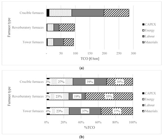
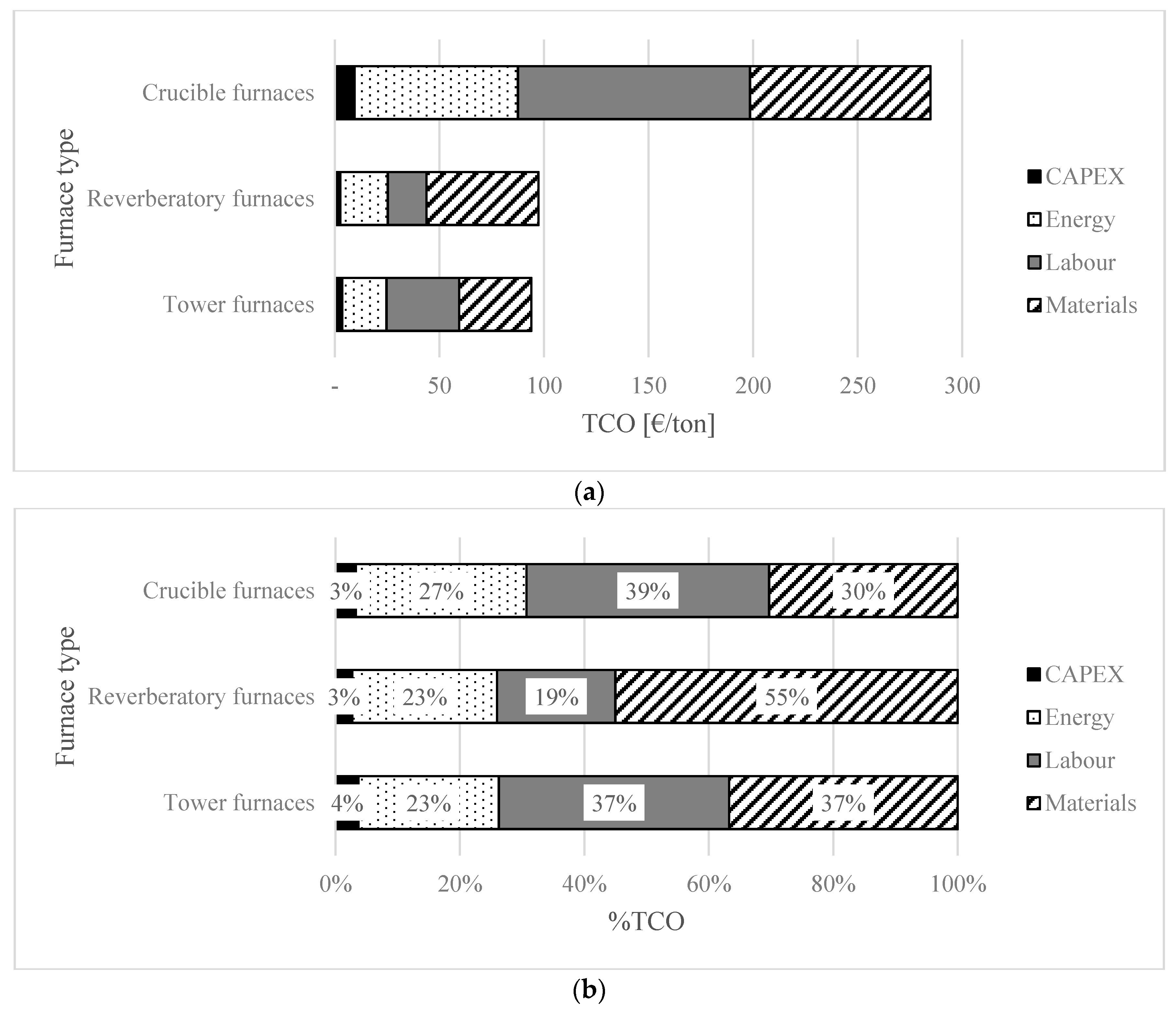
Figure 1 shows the TCO breakdown resulting from the case studies. On average, tower and reverberatory furnaces have the lowest costs among the sample, as they account for 93.94 and 97.31 [€/ton], respectively. Interestingly, the two furnace categories have significantly different cost structures.

Figure 1. Furnaces TCO breakdown, from top to bottom: (a) absolute values; and (b) percentage values.

In particular, the labour cost of tower furnaces (34.75 [€/ton]) is roughly double that of reverberatory furnaces (18.50 [€/ton]): this is mostly explained by the higher complexity of tower furnaces, which requires assigning 2–4 Full Time Equivalent employees (FTEs) to furnace operation and supervision activities. On the other hand, the cost of materials consumed by reverberatory furnaces (53.53 [€/ton]) is significantly higher than tower furnaces (34.51 [€/ton]), mainly due to different melting losses: on average, 4.9–5.3% of the input metal charge is lost during the melting process while running a reverberatory furnace, whereas a tower furnace wastes only 2.5–3.0% of the aluminium received.

Crucible furnaces have the highest TCO among the sample (284.74 [€/ton]). Two major factors contribute to such cost gap. Firstly, the energy consumed by a crucible furnace during the melting process (2.00–2.22 [kWh/kg]) is significantly higher than other gas-fired furnaces (0.68-0.97 [kWh/kg]), which lowers the energy efficiency of crucible furnaces and, in turn, increases their energy cost.

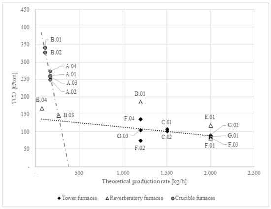
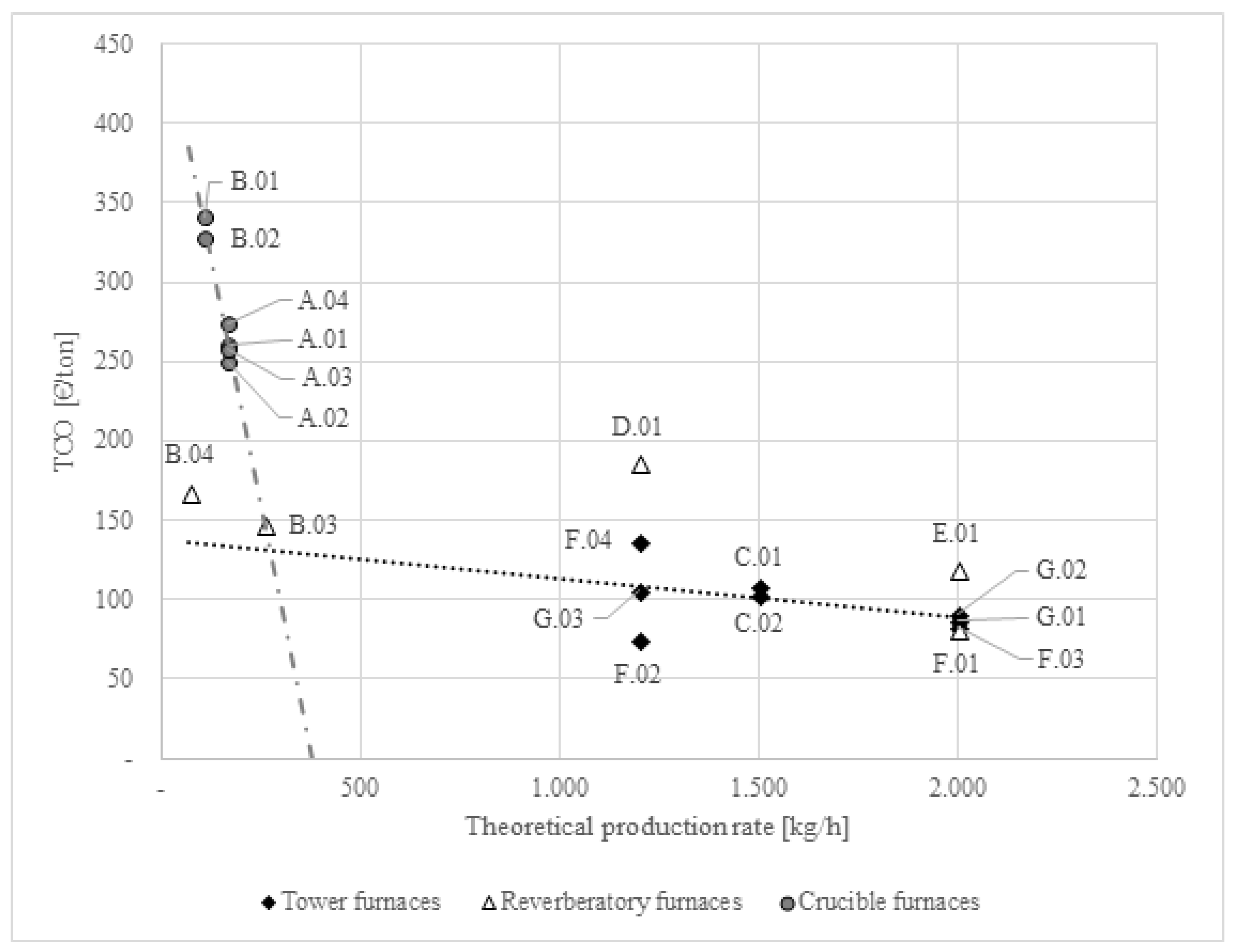
Secondly, the theoretical production rate of crucible furnaces is limited as compared to other gas-fired furnaces. Consequently, crucible furnaces users are less likely to exploit economies of scale of melting aluminium and are considerably impacted by “fixed” costs, such as the cost of labour, as they are independent of the projected output. This effect is highlighted in Figure 2, which shows the correlation between the TCO and the theoretical production rate of the sample furnaces: each furnace is represented by a single point in the scatterplot and is conventionally identified by the company ID (e.g., “A”, “B”, “C”, etc.) and a two-digit progressive number (e.g., “01”, “02”, “03”, etc.).

Figure 2. Correlation between the TCO and the theoretical production rate of the sample furnaces.

These findings indicate that tower furnaces are the best gas-fired melting apparatuses available to aluminium die casting producers.

4.3.2. Production Centralisation

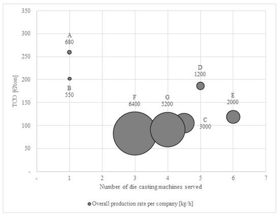
Figure 3 shows the correlation between the number of die casting machines per furnace, the TCO and the overall production rate per company. These results allow classifying the machine layout adopted by the companies in two types:

Figure 3. Correlation between the number of die casting machine per furnace, the TCO and the overall production rate per company.

• Decentralised layout consists of small-sized melting furnaces assigned 1-on-1 to the die casting machines. Only companies A and B adopt this type of layout.
• Centralised layout consists of a set of large-sized melting furnaces serving simultaneously all the available die casting machines. The rest of the sample adopts this layout, which generally implies separating a “foundry department” from the “die-casting department”.

Except for small-sized company D, a cost gap of 80 [€/ton] emerges between companies adopting a decentralized layout and those centralising production in a die-casting department. This result suggests that production centralisation is the cheapest solution, as it allows exploiting more easily the economies of scale of melting aluminium.

However, a comparison of the cost incurred by largest companies C, E, F, and G indicates that distributing the production among a set of two or more large-sized melting furnaces is cheaper than using a single furnace, when adopting a centralised layout.

4.3.3. Molten Aluminium Holding

Selecting the number and the duration of furnace stops is of central importance in optimising the cost of energy consumed by a furnace and, in turn, its TCO. Turning off a furnace allows saving energy to hold the molten aluminium until the production restarts, but implies a “peak” energy consumption to reactivate the furnace, as well. Two distinct approaches have emerged among the sample companies:

• Company B chooses to turn off its crucible furnaces, instead of running them in holding mode, during non-productive time.
• All other companies adopt the opposite policy, i.e., they always run the melting furnaces in holding mode during non-productive time and turn them off only during long-lasting production interruptions, e.g., holiday closings.

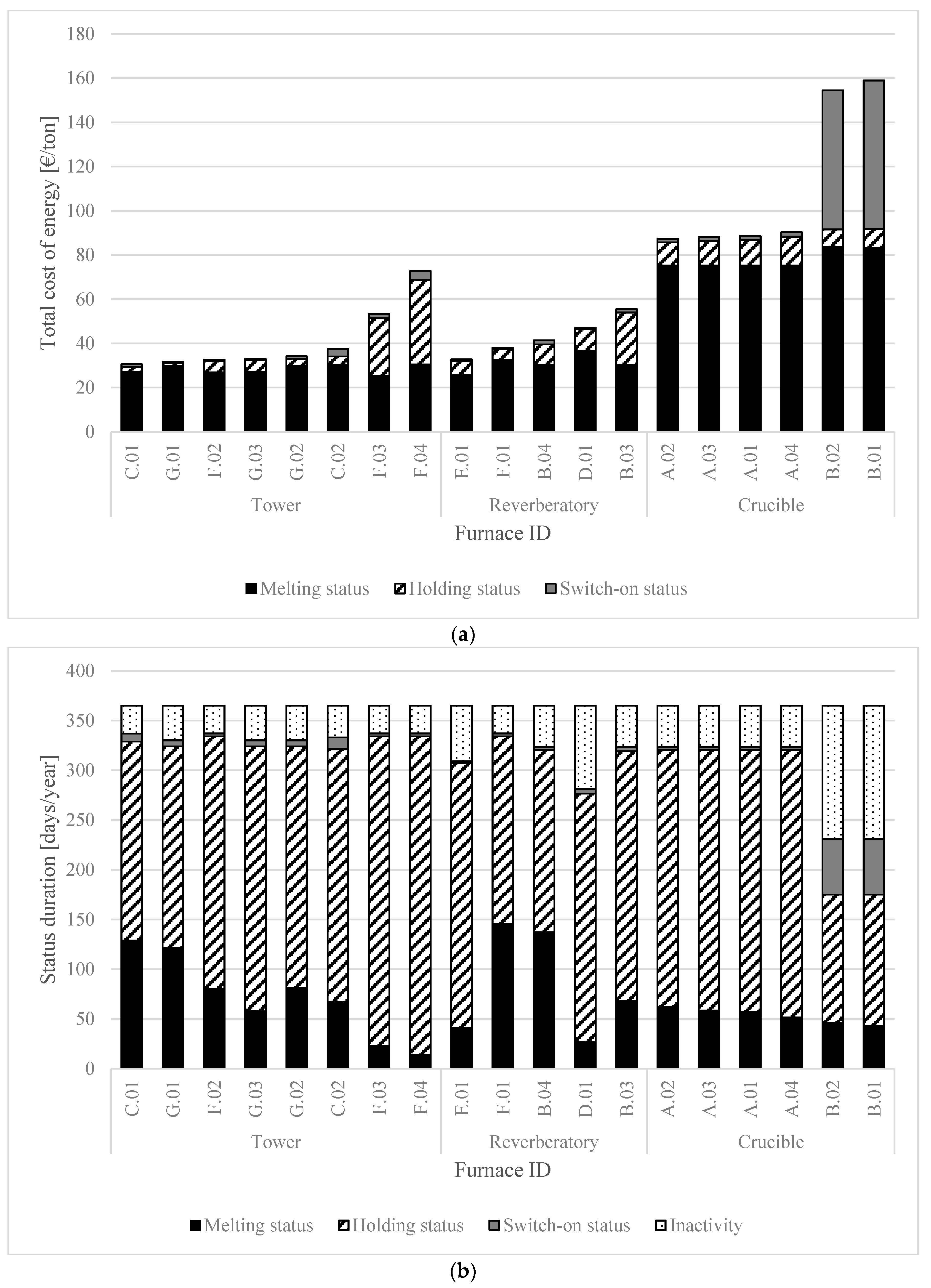
Figure 4 compares the costs of energy consumed by the sample furnaces: a significant cost gap of 64 [€/ton] emerges between crucible furnaces B.01–B.02 and the other furnaces. This suggests that reducing the number of scheduled stops is a cost-effective way to run melting furnaces, even though it implies to keep them in holding status for more than 50% of their lifetime.

Figure 4. Analysis of furnaces statuses, from top to bottom: (a) energy cost; and (b) yearly duration.

In fact, the analysis of furnace statuses duration indicates that aluminium melting furnaces are extensively used for holding purposes: for instance, tower furnaces C.01–G.01 and reverberatory furnaces B.04–F.01 spend about 120–145 [days/year] in melting status, with holding status accounting for 80–85% of the overall non-productive time.

However, scheduling only two stops per year (i.e., summer and Christmas closings) is not always the best solution. For instance, tower furnaces F.03–F.04 spend more than 300 [days/year] in holding status: consequently, their cost of energy is roughly 2–2.5 times that of other tower furnaces. Introducing a third stop or increasing the duration of already scheduled ones, as in the case of reverberatory furnace D.01, could bring to a significant reduction of energy costs.

4.3.4. Working Calendar

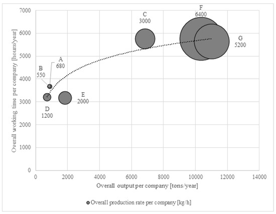
Figure 5 shows the correlation between the overall output, working time and production rate per company. As expected, the results of this analysis indicate that the duration of working calendar is mostly based on the projected output and on the available production capacity.

Figure 5. Correlation between the overall output, working time and production rate of the sample companies.

In particular, large-sized companies C, F and G can afford a three-shift calendar due to considerably high output and production capacity. On the other hand, smaller companies A, B and D adopt a two-shift calendar for the opposite reason. Moreover, company D schedules six weeks more plant closings in an attempt to balance its higher production capacity and lower output than companies A and B. Interestingly, company E adopts an uncommon 12-h shift schedule, as opposed to the standard 8-h shift schedule adopted by the other companies.

Finally, it is worth noting that selecting the work calendar has a significant impact on the cost of energy consumed by a furnace, as it usually runs in holding status during any non-productive shifts.

5. Discussion

The new TCO model developed in this paper, fed with the empirical data collected in the aluminium furnaces case studies, provides some noteworthy findings for selecting, acquiring and reducing operational costs of melting furnaces in the aluminium die casting industry.

At first, managers should look beyond the purchase price when selecting a new melting furnace, and consider also its expected TCO. The empirical results presented in Section 4 show that the CAPEX account for only the 3–5% of a furnace TCO, regardless of its technological features. Moreover, tower and reverberatory furnaces have a significantly lower TCO than gas-fired crucible furnaces, despite having considerably higher purchase prices (90,000–320,000 [€] compared to only 15,000–20,000 [€]). Thus, by considering both the purchase price and the TCO, managers gather a more complete and accurate information in investment decisions on melting furnaces.

Secondly, the melting technology implemented in a furnace highly affects the costs of materials and energy. In particular, tower furnaces are the most efficient gas-fired aluminium melting equipment available to date. These furnaces allow processing high amounts of aluminium with relatively high thermal efficiency (40–48%) and low melting loss (1–2%). Despite being characterised by low flexibility and quite unsuitable to small-scaled production, tower furnaces stand as primary investment options for any aluminium die casting company.

Not surprisingly, the production of molten aluminium relies on economies of scale and adopting a “centralized” machine layout (i.e., a set of melting furnaces serving simultaneously all the available die casting machines) allows a better exploitation of the economies of scale by allowing the adoption of larger furnaces than a “decentralized” one (i.e., melting furnaces assigned 1-on-1 to the die casting machines). Adopting a centralized layout generally implies using the furnaces as molten metal buffers, as the overall production rate of melting furnaces exceeds that of die casting machines. Results indicate that the largest scaled furnaces in the sample spend up to 80–85% of their time in holding status.

At last, minimising the number of scheduled stops seems to be the most effective lever to reduce the operating cost of energy. All the sample companies turn off their furnaces only during holiday closings and emergency maintenance works involving critical components of the furnace (e.g., inner refractory shell, burners, and outer bearing structure). The only exception is company B, which schedules additional stops of its crucible furnaces during alloy changes and incur higher energy costs than its competitor A (98–102 [€/ton] compared to 68–70 [€/ton]).

6. Conclusions

To our best knowledge, the new model presented in this paper comes as the first application of the TCO methodology to aluminium melting furnaces reported in the scientific literature. While this aspect has to be welcome, as it opens up new fruitful research and application perspectives, it entails some conceptual and practical limitations. The current model computes furnace costs based on constant average input data; however, this assumption is at odds with highly dynamic inputs, such as market prices of energy and aluminium, market demand, etc. Secondly, we chose to only focus on the furnaces, implying that the model can only compute the TCO for the foundry Department. Finally, up to now, we could develop a rather limited number of empirical case studies, implying the impossibility to obtain statistically sound conclusions, as well as to perform multi-dimensional analyses.

Despite these limitations, empirical analyses discussed in Section 5 show the new TCO model’s potential to identify the main determinants of furnaces TCO. The empirical data collected and fed to the model allow us to identify, among others, the following drivers:

• the melting technology implemented in the furnace;
• the installed production capacity, in relation to the projected output;
• the machine layout adopted in the foundry and die casting departments; and
• the furnace stop policy chosen by the die casting company.

As such, the model can be used as a sophisticated decision support system, throughout the furnace’s lifecycle. First, the new model can support the selection of a new furnace. Model users can compare the costs of different investment alternatives while simulating plausible operational modes and market prices of energy and aluminium over a projected furnace lifecycle. This simulation can consider the new furnace alone, or the whole furnace department layout, providing the opportunity to configure it for the best.

Secondly, it allows managers to analyse or to simulate the operating costs of melting furnaces. This can be achieved by defining alternative utilisation scenarios applicable to either single or multiple furnaces, e.g., alternative turn-off policies, working calendars and/or production mixes, and evaluate their impact on the TCO of the selected equipment. An in-depth analysis of energy costs allows classifying them in “value-added” (i.e., aluminium melting) and “non-value-added” (e.g., aluminium holding and furnace switch-on) activities. The fluctuation of market prices of energy and aluminium could be taken into account while evaluating the costs of alternative utilisation scenarios, as well. At last, it can support also decommissioning decisions, by comparing the TCO of an “obsolete” furnace currently in operation and an “upgraded” one, although the latter two aspects have not been explored empirically in the case studies.

To overcome the limitations discussed above, future research agenda on this topic should include adopting time-dependent inputs (e.g., time-dependent energy and labour costs), increasing the number of case studies and extending the model to the whole aluminium die casting process. However, we believe the most valuable results will be achieved when the model will allow us to investigate trade-offs between conflicting TCO reduction objectives. Most of the model inputs are interdependent or conflicting with each other and, thus, evaluating the viability of a cost reduction lever is difficult without carrying out multidimensional analyses. For instance, reducing the frequency of routine maintenance works would result in lower turn-off and switch-on costs, but would also expose the furnace itself to higher breakdown costs and reduced lifetime.

References

- Schifo, J.; Radia, J. Theoretical/Best Practice Energy Use in Metalcasting Operations; Office of Energy Efficiency and Renewable Energy, US Department of Energy: Washington, DC, USA, 2004.
- Schwam, D. Final Technical Report: Task 2.1: Melting Efficiency in Die Casting Operations; Department of Materials Science and Engineering: Cleveland, OH, USA, 2004. [Google Scholar]
- Ellram, L.M.; Siferd, S.P. Purchasing: The Cornerstone of the Total Cost of Ownership Concept. J. Bus. Logist. 1993, 14, 163. [Google Scholar]
- AREMA. Manual for Railway Engineering; AREMA: Lanham, Maryland, 2013. [Google Scholar]
- Grant, E.L.; Ireson, W.G. Principles of Engineering Economy; Ronald Press Company: New York, NY, USA, 1970. [Google Scholar]
- Miller, M.H.; Upton, C.W. Leasing, buying, and the cost of capital services. J. Finance 1976, 31, 761–786. [Google Scholar] [CrossRef] [Scilit]
- Goodall, G. TCO: What’s Old Is New. Info-Tech Insight, March. Processor 2008, 30, 24. [Google Scholar]
- Ellram, L.M. A Framework for Total Cost of Ownership. Int. J. Logist. Manag. 1993, 4, 49–60. [Google Scholar] [CrossRef] [Scilit]
- Degraeve, Z.; Roodhooft, F. Determining sourcing strategies: A decision model based on activity and cost driver information. J. Oper. Res. Soc. 1998, 49, 781–789. [Google Scholar] [CrossRef] [Scilit]
- Degraeve, Z.; Roodhooft, F. Improving the efficiency of the purchasing process using total cost of ownership information: The case of heating electrodes at Cockerill Sambre S.A. Eur. J. Oper. Res. 1999, 112, 42–53. [Google Scholar] [CrossRef] [Scilit]
- Degraeve, Z.; Labro, E.; Roodhooft, F. An evaluation of vendor selection models from a total cost of ownership perspective. Eur. J. Oper. Res. 2000, 125, 34–58. [Google Scholar] [CrossRef] [Scilit]
- Degraeve, Z.; Roodhooft, F.; Van Doveren, B. The use of total cost of ownership for strategic procurement: A company-wide management information system. J. Oper. Res. Soc. 2005, 56, 51–59. [Google Scholar] [CrossRef] [Scilit]
- Heinemann, T.; Kaluza, A.; Thiede, S.; Ditterich, D.; Linzbach, J.; Herrmann, C. Life Cycle Evaluation of Factories: The Case of a Car Body Welding Line with Pneumatic Actuators. In IFIP Advances in Information and Communication Technology; Springer: Berlin/Heidelberg, Germany, 2014. [Google Scholar]
- DeGarmo, E.P.; Black, J.T.; Kohser, R.A. DeGarmo’s Materials and Processes in Manufacturing, 11th ed.; John Wiley & Sons: Hoboken, NJ, USA, 2011. [Google Scholar]
- American Foundry Society. 50th census of world casting production. Global Casting Production Stagnant. Mod. Cast. 2016, 25–29. [Google Scholar]
- Schwam, D. Energy Saving Melting and Revert Reduction Technology: Melting Efficiency in Die Casting Operations; Department of Materials Science and Engineering, Case Western Reserve University: Cleveland, OH, USA, 2012. [Google Scholar]
- Ferrin, B.G.; Plank, R.E. Total Cost of Ownership Models: An Exploratory Study. J. Supply Chain Manag. 2002, 38, 18–29. [Google Scholar] [CrossRef] [Scilit]
- Bhutta, K.S. Research paper Supplier selection problem: A comparison of the total cost of ownership and analytic hierarchy process approaches. Supply Chain Manag. 2002, 7, 126–135. [Google Scholar] [CrossRef] [Scilit]
- Caniato, F.; Ronchi, S.; Luzzini, D.; Brivio, O. Total cost of ownership along the supply chain: A model applied to the tinting industry. Prod. Plan. Control. 2015, 26, 427–437. [Google Scholar] [CrossRef] [Scilit]
- Saccani, N.; Perona, M.; Bacchetti, A. The total cost of ownership of durable consumer goods: A conceptual model and an empirical application. Int. J. Prod. Econ. 2017, 183, 1–13. [Google Scholar] [CrossRef] [Scilit]
- Ellram, L.M. Total cost of ownership: An analysis approach for purchasing. Int. J. Phys. Distrib. Logist. Manag. 1995, 25, 4–23. [Google Scholar] [CrossRef] [Scilit]
- Tibben-Lembke, R.S. The Impact of Reverse Logistics on the Total Cost of Ownership. J. Mark. Theory Pract. 1998, 6, 51–60. [Google Scholar] [CrossRef] [Scilit]
- Wouters, M.; Anderson, J.C.; Wynstra, F. The adoption of total cost of ownership for sourcing decisions—A structural equations analysis. Account. Organ. Soc. 2005, 30, 167–191. [Google Scholar] [CrossRef] [Scilit]
- Cavinato, J.L. A Total Cost/Value Model for Supply Chain Competitiveness. J. Bus. Logist. 1992, 13, 285. [Google Scholar]
- Humphries, J.; McCaleb, B. Optimizing Total Cost of Ownership. Plant. Eng. 2004, 58, 23–27. [Google Scholar]
- Gilmore, E.A.; Lave, L.B. Comparing resale prices and total cost of ownership for gasoline, hybrid and diesel passenger cars and trucks. Transp. Policy 2013, 27, 200–208. [Google Scholar] [CrossRef] [Scilit]
- Fischer, R.; Lugg, R. The real cost of ILS ownership. Bottom Line 2006, 19, 111–123. [Google Scholar] [CrossRef] [Scilit]
- Sohn, S.Y.; Lee, J.S. Cost of ownership model for a CRM system. Sci. Comput. Program. 2006, 60, 68–81. [Google Scholar] [CrossRef] [Scilit]
- De Alfonso, C.; Caballer, M.; Alvarruiz, F.; Moltó, G. An economic and energy-aware analysis of the viability of outsourcing cluster computing to a cloud. Future Gener. Comput. Syst. 2013, 29, 704–712. [Google Scholar] [CrossRef] [Scilit]
- Walterbusch, M.; Martens, B.; Teuteberg, F. Evaluating cloud computing services from a total cost of ownership perspective. Manag. Res. Rev. 2013, 36, 613–638. [Google Scholar] [CrossRef] [Scilit]
- Thompson, J.S.; Khirallah, C.; Rashvand, H. Energy and cost impacts of relay and femtocell deployments in long-term-evolution advanced. IET Commun. 2011, 5, 2617–2628. [Google Scholar] [CrossRef] [Scilit]
- Goudarzi, P. Stochastic total cost of ownership optimization for video streaming services. Telemat. Inform. 2014, 31, 79–90. [Google Scholar] [CrossRef] [Scilit]
- Levä, T.; Mazhelis, O.; Suomi, H. Comparing the cost-efficiency of CoAP and HTTP in Web of Things applications. Decis. Support Syst. 2014, 63, 23–38. [Google Scholar] [CrossRef] [Scilit]
- Al-alawi, B.M.; Bradley, T.H. Total cost of ownership, payback, and consumer preference modeling of plug-in hybrid electric vehicles. Appl. Energy 2014, 103, 488–506. [Google Scholar] [CrossRef] [Scilit]
- Le Duigou, A.; Guan, Y.; Amalric, Y. On the competitiveness of electric driving in France: Impact of driving patterns. Renew. Sustain. Energy Rev. 2014, 37, 348–359. [Google Scholar] [CrossRef] [Scilit]
- Ragona, S. Cost of ownership (COO) for optoelectronic manufacturing equipment. In Proceedings of the 2002 Microsystems Conference, Rochester, NY, USA, 22–25 September 2002. [Google Scholar]
- Heilala, J.; Helin, K.; Montonen, J. Total cost of ownership analysis for modular final assembly systems. Int. J. Prod. Res. 2006, 44, 3967–3988. [Google Scholar] [CrossRef] [Scilit]
- Nahas, N.; Nourelfath, M.; Gendreau, M. Selecting machines and buffers in unreliable assembly/disassembly manufacturing networks. Int. J. Prod. Econ. 2014, 154, 113–126. [Google Scholar] [CrossRef] [Scilit]
- Heinemann, T.; Schraml, P.; Thiede, S.; Eisele, C.; Herrmann, C.; Abele, E. Hierarchical evaluation of environmental impacts from manufacturing system and machine perspective. Procedia CIRP 2014, 15, 141–146. [Google Scholar] [CrossRef] [Scilit]
- Trybula, W. Cost of ownership—Projecting the future. Microelectron. Eng. 2006, 83, 614–618. [Google Scholar] [CrossRef] [Scilit]
- Thiede, S.; Spiering, T.; Kohlitz, S. Dynamic Total Cost of Ownership (TCO) Calculation of Injection Moulding Machines. In Leveraging Technology for a Sustainable World; Springer: Berlin/Heidelberg, Germany, 2012. [Google Scholar]
- Chen, S.; Keys, L.K. A cost analysis model for heavy equipment. Comput. Ind. Eng. 2009, 56, 1276–1288. [Google Scholar] [CrossRef] [Scilit]
- Renquist, J.V.; Dickman, B.; Bradley, T.H. Economic comparison of fuel cell powered forklifts to battery powered forklifts. Int. J. Hydrogen Energy 2012, 17, 12054–12059. [Google Scholar] [CrossRef] [Scilit]
- Noll, P. Determining the real cost of powering a pump. World Pumps 2008, 496, 32–34. [Google Scholar] [CrossRef] [Scilit]
- Mader, G.; Madani, H. Capacity control in air-water heat pumps: Total cost of ownership analysis. Energy Build. 2014, 81, 296–304. [Google Scholar] [CrossRef] [Scilit]
- Sohn, S.Y.; Kim, Y.; Kim, B.T. Cost of ownership model for spare engines purchase for the korean navy acquisition program. J. Oper. Res. Soc. 2009, 60, 1674–1682. [Google Scholar] [CrossRef] [Scilit]
- Ramadan, S.Z. Selection of non-repairable series systems’ components with Weibull-life and lognormal-repair distributions through minimizing expected total cost of ownership approach. Mod. Appl. Sci. 2014, 8, 104. [Google Scholar] [CrossRef] [Scilit]
- Holmquist, J.R. Reasons for using IEEE Standard 841-1994 motors for the forest products industry. In Proceedings of the Pulp and Paper Industry Technical Conference, Portland, ME, USA, 21–26 June 1998; pp. 87–96. [Google Scholar]
- Kumar, U.D.; Saranga, H. Optimal selection of obsolescence mitigation strategies using a restless bandit model. Eur. J. Oper. Res. 2010, 200, 170–180. [Google Scholar] [CrossRef] [Scilit]
- Ellram, L.M. Activity-based costing and total cost of ownership: A critical linkage. Cost Manag. 1995, 8, 22–30. [Google Scholar]
- Hurkens, K.; van der Valk, W.; Wynstra, F. Total cost of ownership in the services sector: A case study. J. Supply Chain Manag. 2006, 42, 27–37. [Google Scholar] [CrossRef] [Scilit]
© 2018 by the authors. Licensee MDPI, Basel, Switzerland. This article is an open access article distributed under the terms and conditions of the Creative Commons Attribution (CC BY) license (http://creativecommons.org/licenses/by/4.0/).