Article

Variability of Satellite Derived Phenological Parameters across Maize Producing Areas of South Africa

1
Department of Geography, Geoinformatics & Meteorology, University of Pretoria, Private Bag X20, Hatfield, Pretoria 0028, South Africa
2
South African Weather Service, Private Bag X097, Pretoria 0001, South Africa
3
Department of Animal and Wildlife Sciences, University of Pretoria, Private Bag X20, Hatfield, Pretoria 0028, South Africa
4
Department of Plant and soil Sciences, University of Pretoria, Private Bag X20, Hatfield, Pretoria 0028, South Africa
5
Department of Agricultural and Applied Economics, Texas Tech University, Lubbock, TX 79409, USA
*
Author to whom correspondence should be addressed.
Sustainability 2018, 10(9), 3033; https://doi.org/10.3390/su10093033
Submission received: 21 June 2018 / Revised: 19 July 2018 / Accepted: 31 July 2018 / Published: 27 August 2018
(This article belongs to the Section Sustainable Agriculture)

Abstract

:
Changes in phenology can be used as a proxy to elucidate the short and long term trends in climate change and variability. Such phenological changes are driven by weather and climate as well as environmental and ecological factors. Climate change affects plant phenology largely during the vegetative and reproductive stages. The focus of this study was to investigate the changes in phenological parameters of maize as well as to assess their causal factors across the selected maize-producing Provinces (viz: North West, Free State, Mpumalanga and KwaZulu-Natal) of South Africa. For this purpose, five phenological parameters i.e., the length of season (LOS), start of season (SOS), end of season (EOS), position of peak value (POP), and position of trough value (POT) derived from the MODIS NDVI data (MOD13Q1) were analysed. In addition, climatic variables (Potential Evapotranspiration (PET), Precipitation (PRE), Maximum (TMX) and Minimum (TMN) Temperatures spanning from 2000 to 2015 were also analysed. Based on the results, the maize-producing Provinces considered exhibit a decreasing trend in NDVI values. The results further show that Mpumalanga and Free State Provinces have SOS and EOS in December and April respectively. In terms of the LOS, KwaZulu-Natal Province had the highest days (194), followed by Mpumalanga with 177 days, while North West and Free State Provinces had 149 and 148 days, respectively. Our results further demonstrate that the influences of climate variables on phenological parameters exhibit a strong space-time and common covariate dependence. For instance, TMN dominated in North West and Free State, PET and TMX are the main dominant factors in KwaZulu-Natal Province whereas PRE highly dominated in Mpumalanga. Furthermore, the result of the Partial Least Square Path Modeling (PLS-PM) analysis indicates that climatic variables predict about 46% of the variability of phenology indicators and about 63% of the variability of yield indicators for the entire study area. The goodness of fit index indicates that the model has a prediction power of 75% over the entire study area. This study contributes towards enhancing the knowledge of the dynamics in the phenological parameters and the results can assist farmers to make the necessary adjustment in order to have an optimal production and thereby enhance food security for both human and livestock.

1. Introduction

Phenology studies the seasons and cycles of natural phenomena controlled by both climatic and environmental factors [1]. It determines the duration and time taken by a plant canopy to be photosynthetically active and equally drives the annual uptake of carbon in an ecosystem [2,3]. It also indicate long-term trends in climate as well as short-term climatic variation as it is driven by precipitation, photoperiod and temperature [4]. Climate change occurs at both global and regional level and it significantly affects vegetation dynamics through the increasing global mean temperature and change in the precipitation regimes [5]. Consequently, climate change affects plant phenology due to its influence on the flowering time and the other plant developmental stages [6]. The changes in vegetation phenology in the past decades, detected from both ground observation and satellite remote sensing phenological methods, have drastically drawn the attention of the scientific community to plant phenology [7,8].
Although first-hand phenology information is assessed with the ground observation phenological methods [9], the major hitch of these methods is that they are localized, lacking global coverage, covering a limited number of species and are highly labour intensive [10]. However, modern remote-sensing techniques provide a promising option and new opportunities for phenological studies [11], since it allows the usage of global coverage data at various spatial and temporal scales, making it easy to study phenology and its drivers. Phenological products have been proven to be useful and have been applied in many fields, like biomass monitoring [12,13], farm management [14,15], and climate change [16,17,18,19,20]. In the past two decades, the usage of satellites to determine vegetation phenology has been an active area of research [8]. Evident in the numerous studies at local and global scales, arrays of algorithms and techniques that handle wide-ranging spatial resolution and temporally discontinuous satellite data have emerged [20]. Remotely sensed vegetation phenological metrics such as Vegetation Indexes (VIs) are derived from satellite time-series data of vegetation parameters. The VIs are among the mostly used parameters and these comprise of the Enhanced Vegetation Index (EVI) [21,22] and the Normalized Difference Vegetation Index (NDVI) [23]. Some other vegetation indices that indicate the growing seasonal changes explored in many studies include: Meris Terrestrial Chlorophyll Index (MTCI) [24], Wide Dynamic Range Vegetation Index (WDRVI) [25], Perpendicular Vegetation Index (PVI) [23] and Soil Adjusted Vegetation Index (SAVI) [26].
NDVI is the measurement of vegetation greenness using a remote-sensing technique, it is associated to the plant’s structural properties such as the green biomass [27] as well as the leaf area index [28] and also relates to properties of vegetation productivity that are the absorbed foliar nitrogen and the absorbed photosynthetic active radiation [29]. As reported by Reference [30], the physiological response of crops to environment conditions, as well as their biophysical characteristics change seasonally as vegetation grows. Information on the phenological stage of a crop is essential for understanding the seasonal exchange of ecosystem carbon dioxide (CO2), fertilizer management, evaluating crop productivity and irrigation scheduling. Maize is the focus of this study and it is a major livestock feed and stable food in South Africa. The reproductive stage which is from sulking to physiological maturity (degree of kernel development), and the vegetative stage which is from emergence to tasselling (number of fully expanded leaves), requires the optimal supply of nutrients under favourable environmental conditions (that is solar radiation, precipitation, soil moisture, temperature), for maximum yield [31,32]. Previous studies [33,34,35] have shown that sustainable development in Southern Africa is threatened by extreme conditions such as water availability (precipitation), rise in air temperature as well as shortening of the length of the growing season. Also, records show that agricultural production in 2015/16 reduced by 1.6% compared to that of 2014/15 [34], also there is reduction in the field crop volume by 12.7%, resulting in a reduction of winter crop production (canola and wheat), summer crops (sorghum and maize), sugar cane and oilseed crops (groundnuts and soya beans) [36].
The analysis of the variability of the phenological parameters induced by climate change and variability can allow for more accurate prediction of the timing of planting crops and help improve managerial decisions, through the provision of phenological parameters (such as: start of season (SOS), end of season (EOS), length of the season (LOS), and maximum NDVI during the season). This study aims at investigating the changes in the phenology metrics in and the associated changes in maize yield and the potential causal factors across the four major producing Provinces of South Africa, namely North West (NW), Free State (FS), Mpumalanga (MP) and KwaZulu-Natal (KZN). The specific objectives of the study are, (a) to calculate the temporal trends of the phenological parameters, (b) to assess the possible association of the changes in phenological parameters with changes in maize yield, and (c) to identify the most significant drivers of such phenological parameters-maize yield changes.

2. Materials and Method

2.1. Study Area

The study area covers the north-eastern part of South Africa between longitude 22° E to 33° E and latitude −32° S to −24° S. The region covers KwaZulu-Natal, Free State, Mpumalanga and North West Provinces; see Figure 1. These Provinces account for approximately 83% of the total maize production for South Africa. FS and NW Provinces together contribute more than 60% of the total maize produced in the country, followed by MP (~24%) and KZN (less than 5%). Free State is about 1300 m above sea level and is characterized by a hot and arid climate. This Province is characterized by chilly winters (ranging from a cold 1 °C to mild 17 °C), plenty of sunshine (15 °C to 32 °C) and summer rains (500 mm–600 mm annually). Located in the northern part of the country, is the Vaal irrigated area which nourishes the small assortment of farming towns. In NW Province there is almost a year-round sunshine, with an average rainfall of 300 to 700 mm annually. The summer temperature ranges from 22 °C to 34 °C. The NW Province is characterized by dry, sunny days and chilly nights during winter (2 °C to 20 °C). The temperature in KZN ranges between 23 °C to 33 °C in summer (i.e., September–April), and 16 °C to 25 °C during winter. The Province is characterized by long, hot summers with average annual rainfall ranging between 500 mm and 800 mm, and mild winters. Furthermore, the western part of MP Province is much colder during winter and hotter during summer than the other parts of the Province. The average annual temperature is about 19 °C and rainfall is between 500 mm and 800 mm annually.

2.2. Materials

A 16-day NDVI composite from MODIS (MOD13Q1) data on board the TERRA and AQUA satellites, with a spatial resolution of 250 m, was acquired from Land Processes Distributed Active Archive Centre (LP DAAC) located at United States Geological Survey (USGS) Earth Resource Observation and Science (EROS) centre for the period of 2000 to 2015. This data is designed in such a way that a variety of information ranging from oceanic conditions to atmospheric and land conditions can be retrieved from it. MOD13Q1 is one of the 44 products (that is processed data) developed by the MODIS science team using a large number of spectral bands.
Maize production data sets in tonnes (tons) for the major maize-producing Provinces spanning from 2000 to 2015 were obtained from the Abstract of Agricultural Statistics compiled by the Department of Agriculture, Forestry and Fisheries of South Africa. This abstract document contains important information on inter alia, field crops, horticulture, livestock, vital indicators, total land area in hectares (ha) cultivated for maize production, and the contribution of primary agriculture to the South African economy. The analysed data are available on the department’s website (www.daff.gov.za).
Gridded climate dataset, of the Climate Research Unit Time-Series 3.24.01 (CRU TS 3.24.01) spanning the period 1986–2015 was used in this study. The CRU TS climate data sets are derived from monthly observations from more than 4000 meteorological stations distributed across the world’s land areas. The gridded CRU TS 3.24.01 product is freely available for the science community on http://www.cru.uea.ac.uk or http://badc.nerc.ac.uk/data/cru. For more information on the construction of the CRU TS 3.24.01 product, the reader is referred to Reference [37]. For the purpose of this study, four climatic variables i.e., precipitation (PRE), maximum and minimum temperature, (TMX) and (TMN) and potential evapotranspiration (PET) spanning the period of 2000–2015 were analyzed. The PET was calculated based on the Penman-Monteith formula reported in e.g., Howard Penman and John Monteith [38].

2.3. Methods

MODIStsp, a new “R” package that allows generation of time series of rasters automatically from Land Products data [38] derived from MODIS satellite data was used to acquire the MODIS NDVI (MOD13Q1) data [39]. The NDVI was derived from spectral measurement of the MODIS sensor using Equation (1).
N D V I = ( N I R R e d ) ( N I R + R e d )
In Equation (1), NIR represents the near-infrared regions while Red represents the spectral reflectance measurements required in the red (visible). The NDVI varies between −1.0 and +1.0. The MOD13Q1 data are provided every 16 days at 250-m spatial resolution as a gridded level-3 product in the Sinusoidal projection. The spatial extent was set by uploading the spatial file for South Africa so as to extract the data for South Africa and thereafter extract the NDVI data for the four major maize-producing Provinces. A comprehensive procedure of downloading and extracting the MODIS data is described in Reference [38].
The output was processed using the greenbrown package in R software (version 2.2) [40] to calculate the phenology metrics on time series from the start of season (SOS), end of season (EOS), length of season (LOS), position of peak (POP), position of trough (POT), spanning from 2000 to 2015. The phenological parameters analysed in this study are summarised in Table 1.
The statistical characteristics of the NDVI and derived phenological parameters were calculated for the purpose of obtaining statistical description. The datasets were de-trended using the quadratic polynomial trend to remove fluctuations attributed to non-climatic factors. The Ordinary Least Square (OLS)-based MOSUM [41] test was used to detect the structural changes and the breakpoints in the time series of the datasets. Statistical significance was tested at 95% confidence limit.
In this contribution, we posit that changes in maize yield are linked to the changes in phenological parameters which are driven mainly by climatic factors among other factors. To test this hypothesis, the Partial Least Square Path Modeling (PLS-PM) was used [42]. Hence, we developed a model that consists of three latent variables; Climate = L V 1 , Phenology = L V 2 and Yield = L V 3 . Each latent variable is associated with at least two manifest variables TMN, TMX, PET and PRE for climate, SOS, EOS, LOS, POP and POT for phenology; and production and cultivated land for yield as shown in Figure 2.
The changes in the phenological variables can be considered as reflective indicators because they reflect the variation in climatic factors; considered as a formative indicator because they are thought to influence the quantity of yield. Hence, L V 2 and L V 3 are treated as reflective blocks expressed as
X 2 k = λ 2 k L V 2 + ε   k = 1 , 2 , 3
X 3 k = λ 3 k L V 3 + ε   k = 1 , 2 , 3
and L V 1 as formative block.
L V 1 = k λ j k X 1 k + ε   k = 1 , 2 , 3
where λ j k are loadings; and ε is the error terms accounting for the residuals.
Shown in Figure 2 is the Path Diagram of the PLS model indicating the two sub-models, the inner and the outer model. The inner model has to do with the relationships between the latent variables and the outer model has to do with the relationships between each latent variable and its block of indicators. For the inner model, two equations were developed. The first is the one which L V 2 depends on L V 1 :
L V 2 j = β j i L V 1 i + ε j
The second inner relationship is the one which L V 3 depends on L V 1 and L V 2 :
L V 3 j = β j i L V 1 i + β 32 j i L V 2 i + ε j
where the subscript i of L V i refers to all the latent variables that are supposed to predict L V j . The coefficients β j i are the path coefficients and they represent the “strength and direction” of the relations between the response L V j and the predictors L V i . β o is the intercept term, and ε j is the error term accounting for the residuals. All variables were standardized.
In order to assess the outer model, the unidimensionality function was used. In this regard, the Cronbach’s alpha, Dillon-Goldstein’s rho, as well as first eigenvalue of the indicators’ correlation matrix were computed. Additionally, the structural model was assessed by computing the R2 determination coefficients, the redundancy index, and the Goodness-of-Fit (GoF).

3. Results

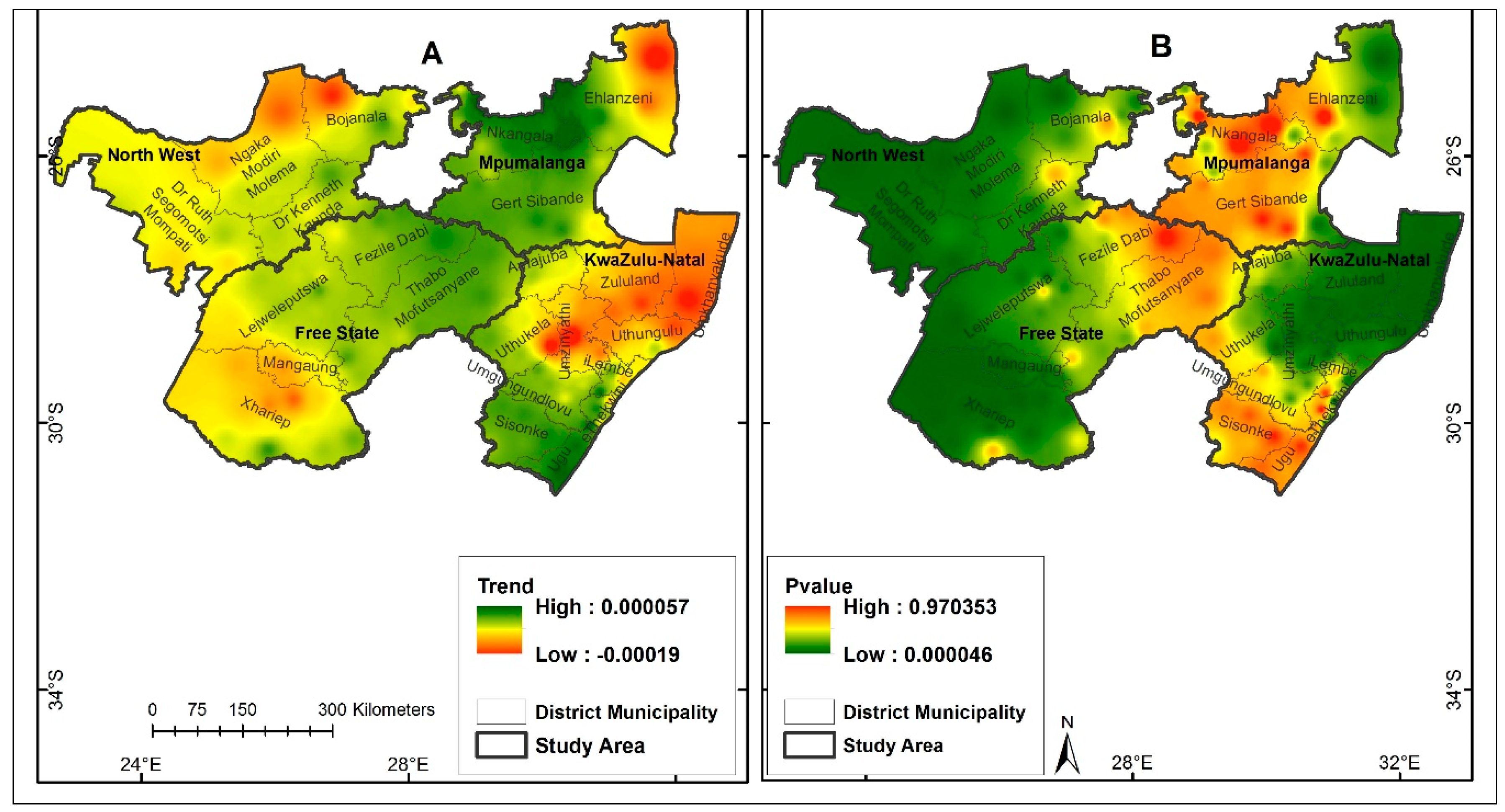
3.1. Summary Statistics and Trends in MODIS Derived NDVI

NDVI statistical characteristics results for the period spanning 2000–2015, are depicted in Table 2. The highest maximum (0.71), minimum (0.35) and median (0.56) NDVI values were recorded in KZN Province while the lowest maximum (0.52), minimum (0.21) and median (0.31) NDVI values were recorded in the NW Province. The variation of NDVI values is high in FS (coefficient of variation; CV = 26.33), NW (CV = 25.93) and MP (CV = 25.55) Provinces and less in KZN (CV = 19.13). The trends of the NDVI time series (black), seasonally adjusted and fitted with the NDVI data (green) are illustrated in Figure 2, while Figure 3 depicts the spatial pattern of trends and p-values of the NDVI over the period of the study.
Generally, negative trends that are statistically significant at α = 5% (p-value = 0.01) were detected in the monthly NDVI values in all the four Provinces. As shown in Figure 3, there were breakpoints in the time series in the month of July 2009 in the FS Province, January 2004 in Mpumalanga Province and July 2008 and June 2012 in North West and KZN Provinces, respectively.
Positive trends (green) were detected in the north and central regions, towards the southern part of the study area consisting of district municipalities such as Nkangala, Gert Sibande in Mpumalanga Province, Fezile Dabi, Thabo Mofutsanyane and Lejweleptswa in Free State Province, and in Umgungundlovu, Sisonke and Ugu in KwaZulu-Natal; see Figure 4A. However, the observed trends are not statistically significant, see for instance Figure 4B. On the other hand, negative trends in NDVI values were detected in the north-eastern parts of Ngaka Modiri Molema and the north-western regions of Bojanala districts in the north-eastern parts of North West Province; north-eastern parts of Ehlanzeni in Mpumalanga Province as well as in the central and north-eastern parts of KwaZulu-Natal Province. The negative trends are statistically significant are shown in Figure 4B.

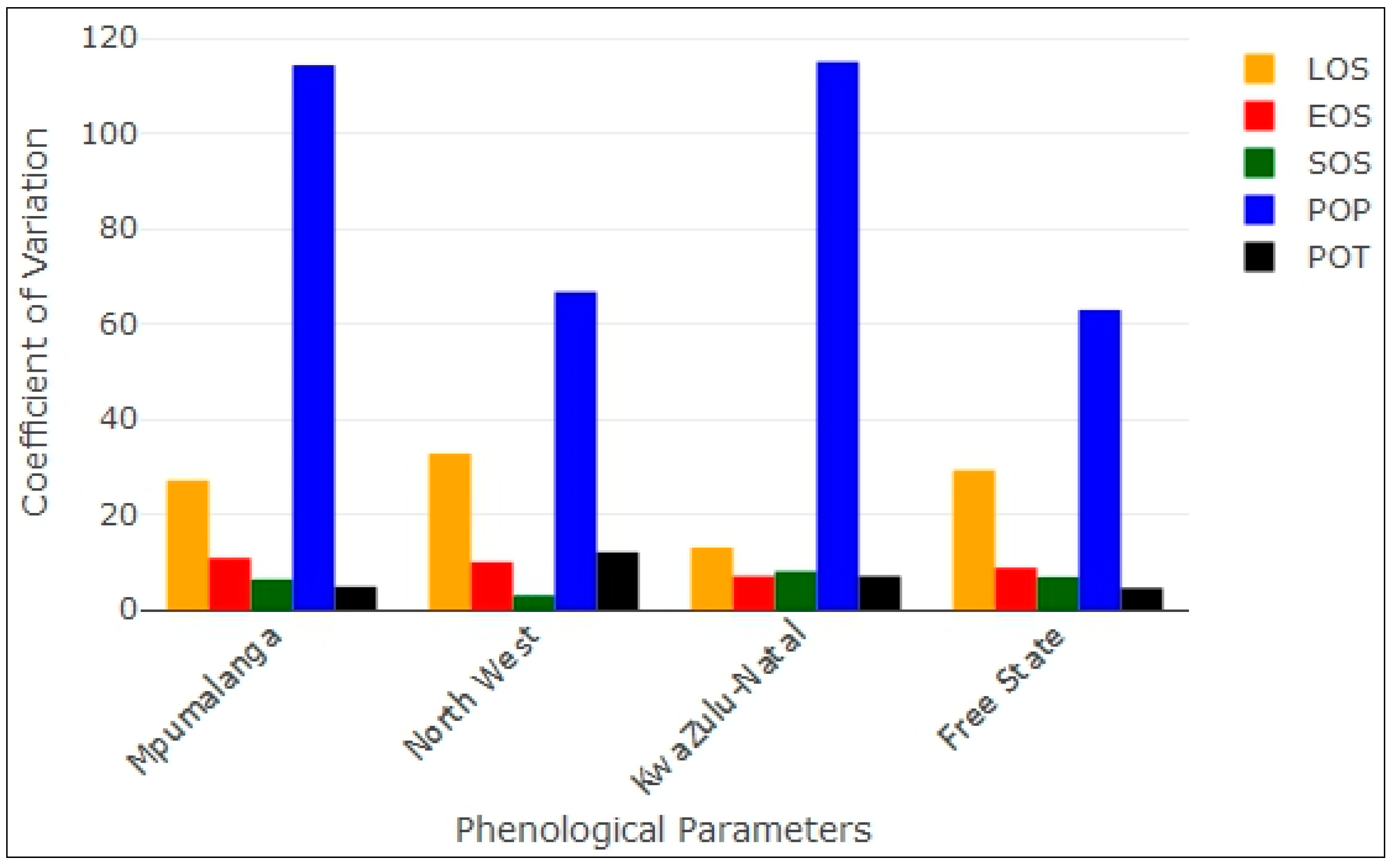
3.2. Statistical Moments of Phenological Parameters

Figure 5 depicts the statistical characteristics of the phenological parameters across the study area. Based on the results, the SOS ranges between the 260th and 359th day of the year, with noticeable outliers in KZN. Over the 17-year period, the North West Province exhibited an SOS median value of the 336th day of the year which falls in December and ends (EOS) on the 120th day of the following year (April), while the LOS median value is approximately 166 days. The NDVI peak value (position of peak value (maximum) (POP)) was attained on the 38th day of the year (i.e., around February) while the NDVI trough value (position of trough value (minimum) (POT)) was attained on the 225th day of the year, which is around August. The mean growing season NDVI (MGS) value for North West Province is 0.42. In Mpumalanga Province, the median SOS falls on the 304th day of the year (corresponding to days in November), the median EOS is on the 111th day of the following year (around April) while the median LOS is approximately at about 178 days. The peak NDVI value (POP) occurs around the 14th day of the year (around January) while the trough NDVI value (POT) is determined to be around the 215th day of the year (around August). The MGS value for Mpumalanga Province is 0.58. The growing season for KwaZulu-Natal Province starts on around the 293rd day of the year (October), and ends on the 126th day of the following year (May). The LOS stretches for about 196 days. The maximum NDVI value is detected on the 19th day of the year (January) while the minimum NDVI value occurs around the 203rd day of the year (July). The MGS value for KwaZulu-Natal is 0.63. In Free State, the season starts (SOS) on the 319th day of the year, which is in November, and ends (EOS) on the 114th day of the following year (April), the LOS stretches for about 151 days. The MGS value for this area is 0.42. The maximum NDVI value was detected on the 35th day of the year (around February) while the minimum NDVI value was on the 193rd day of the year (July).
The graphical illustration of the phenological parameters is shown in Figure 6. From this figure, it is evident that the planting season starts (SOS) late in the North West and Free State Provinces as compared to the other two provinces. The growing season for the KwaZulu-Natal and North West Provinces ends late (that is higher EOS values) as compared to other areas. However, the KwaZulu-Natal and Mpumalanga Provinces experienced the longest growing season (higher LOS values). The North West and Free State Provinces exhibited the highest POP values while the North West and Mpumalanga Provinces showed the highest POT values.
Figure 7 depicts results for the computed coefficient of variation (CV). The CV results indicate that the POP exhibited the greatest variability while SOS and POT exhibited the least variability, in all the major maize-producing Provinces of South Africa. However, the POP in KwaZulu-Natal and Mpumalanga varies more than the other two Provinces. The LOS in KwaZulu-Natal had the least variation compared to the rest of the Provinces. And POT in North West varied more than the other Provinces.

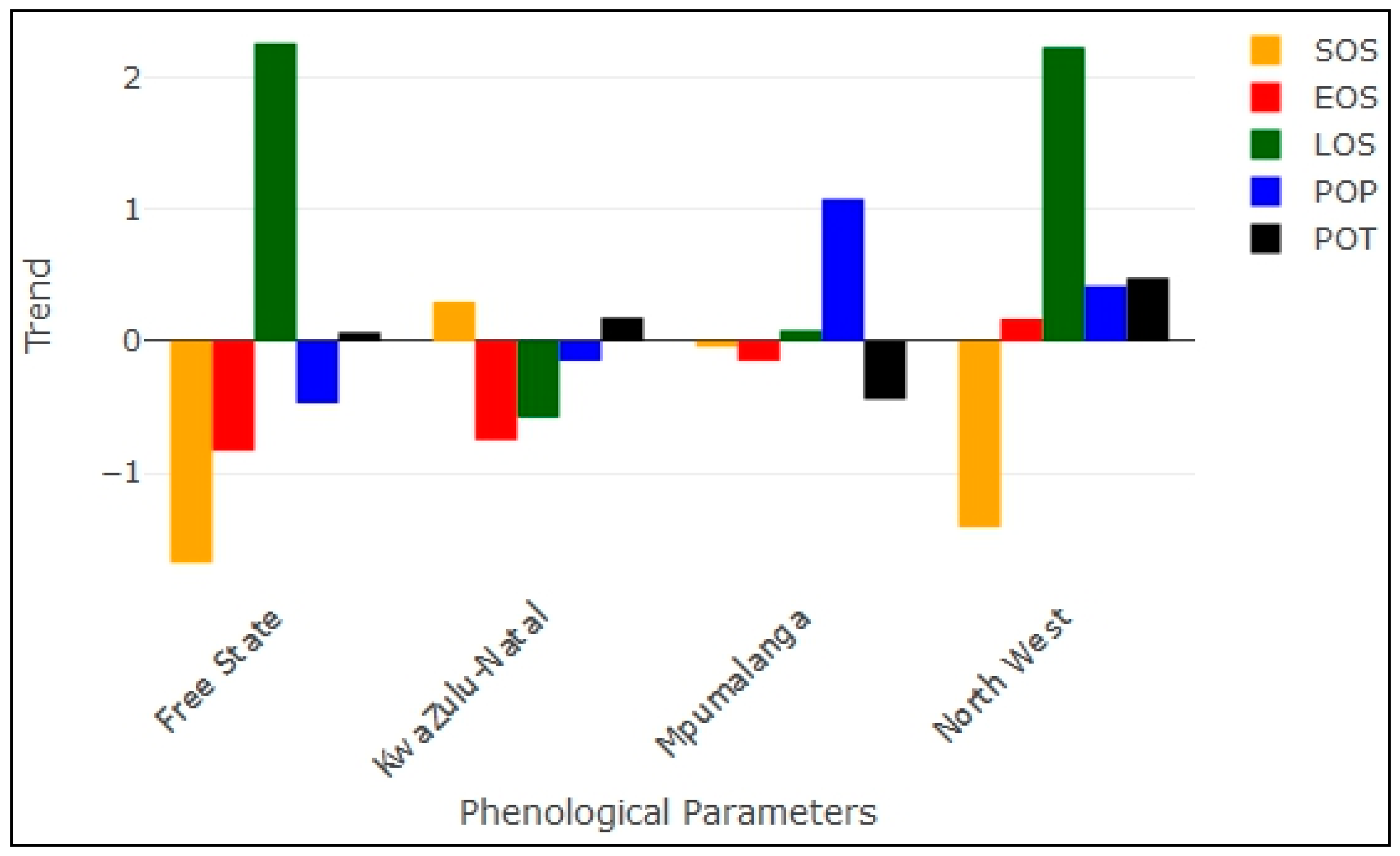
3.3. Trends in the Phenological Parameters from 2000 to 2015

Shown in Figure 8 and Table 3 are the trend in the phenological parameters from 2000 to 2015 as well as the statistical significance of trends in the phenological parameters. Negative trends in the SOS were detected across the entire maize-producing Provinces with exception to KwaZulu-Natal which depicted a positive trend. The SOS exhibited similar trend patterns across all but one (North West) Province. Furthermore, negative trends in EOS were observed across the study area, with exceptions to the North West Province which depicted a positive trend with no significant difference. The LOS exhibited a positive trend in all the Provinces except for KwaZulu-Natal Province, with no significant difference in the LOS for all the Provinces except for North West Province which increased significantly. The POT exhibited a positive trend in all but one (Mpumalanga) Province. On the other hand, POP in Free State and KwaZulu-Natal Provinces showed a negative trend while POP in Mpumalanga and North West Provinces experienced positive trends. Trends in both POT and POP were found to be statistically insignificant across the Provinces.

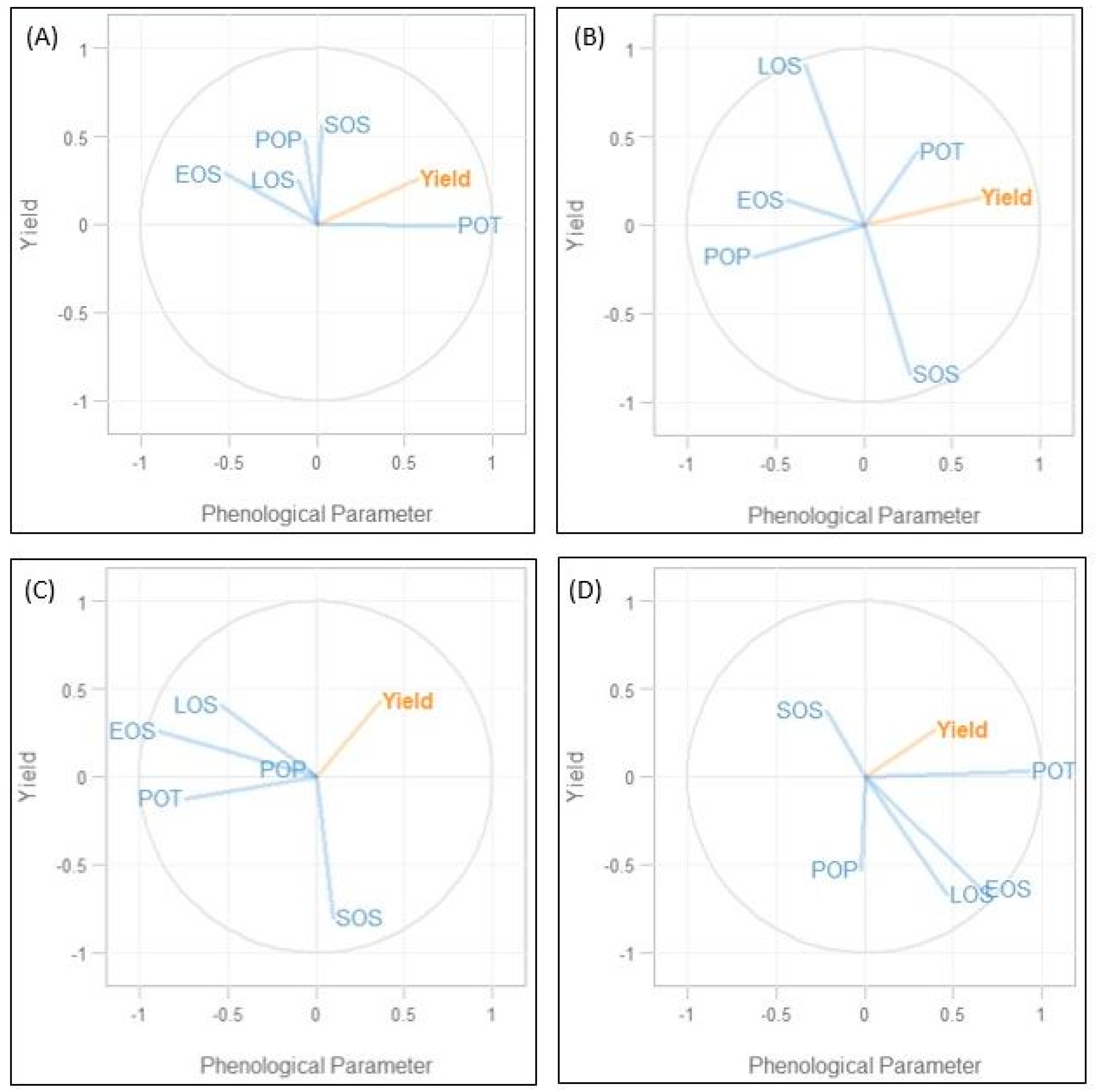
3.4. Association of Changes in Maize Yield and Changes in Phenological Parameter

Considering the circle of correlations for Free State in Figure 9A, POT had the closest correlation with the maize yield. On the other hand, EOS, POP, LOS and SOS had a very strong correlation with each other, although LOS, POP and SOS were poorly represented in the plot while the other phenological parameter were well represented in the circle of correlations plot. This means that the LOS, SOS, EOS and POP for Free State had a very strong relationship. In the circle of correlations for KwaZulu-Natal (Figure 9B), POT also had the greatest influence on the maize yield for the area. However, there exists no correlation among the phenological parameters in the area. And EOS and POT were poorly represented in the plot while the other phenological parameters were well represented in the plot. For Mpumalanga Province (Figure 9C), POP and LOS had a stronger influence on the maize yield than the other phenological parameters. There is also a close relationship between LOS and POP, this means that these parameters influences each other, although POP has less influence as shown in Figure 9C. Maize yield in the North West Province is equally strongly, influenced by POT according to the circle of correlations in Figure 9D. The LOS and the EOS in this Province had a very close relationship suggesting that they influence each other.

3.5. Impact of Varying Phenological Parameter on Maize Yield

In this study, a multivariate analysis model was used to assess the relationships among maize yield, phenological parameters and climatic parameters. The multivariate analysis results are summarized in Table 4. As shown in Table 4, changes in phenological parameters can be associated to variations in the maize yield for the major maize-producing areas ranging from 70% in Mpumalanga, 72% in KwaZulu-Natal, 76% in North West and 79% in Free State.
According to Table 4, from 2000 to 2015, there was an estimated reduction in the maize yield in the North West Province of about 0.01 tons per hectare (t/ha) when the climatic parameters and phenological parameters are held constant at their averages; that is when PET is 5.3 mm/day, PRE is 57 mm/month, TMN is 16 °C, TMX is 31 °C, SOS is on day 339, EOS is on day 117, LOS is 149 days, POP is on day 35 and POT is on day 225. However, a minimal increase of about 1% in the mean value of PET, PRE, and TMN led to an increase of about 0.47, 0.02, 0.30 t/ha in maize yield, respectively, while an increase of about 1% in the mean value of TMX led to a reduction of about 0.05 t/ha in maize yield. On the other hand, at about 1% increase in the mean values of SOS, LOS, POP and POT there was a decrease of about 1.44, 3.49, 1.39 0.89 t/ha of maize yield, respectively; however, EOS increased maize yield by about 3.55 t/ha. In Mpumalanga Province, maize yield decreased by 0.003 t/ha when the phenological parameters are at average values. An increase of about 1% above the average value in PRE (108 mm/month), TMX (25 °C), SOS (day 309), and LOS (day 179) led to a decrease of 0.39 t/ha, 0.35 t/ha, 1.56 t/ha, and 1.74 t/ha in maize yield respectively. However, 1% increase in the average values of PET, TMN, EOS, POP, and POT increased maize yield by 0.46 t/ha, 0.85 t/ha, 0.28 t/ha, 0.05 t/ha and 0.01 t/ha respectively. In KwaZulu-Natal Province, no change in maize yield per hectare was observed when average values of PET, PRE, TMN, TMX, SOS, EOS, LOS, POP and POT are held constant at 3.9 mm/day, 103 mm/month, 15 °C, 27 °C, day 295, day 126, 194 days, day 20 and day 203, respectively. With a 1% increase in the mean values of PET, PRE, SOS, LOS and POT there was an increase of about 0.36 t/ha, 2.92 t/ha, 1.57 t/ha, 1.19 t/ha and 0.82 t/ha in maize yield respectively. However, maize yield reduced by about 0.26, 1.0, 1.24, 0.71 t/ha with 1% increase of the mean values of TMN, TMX, EOS and POP respectively. While in Free State, an increase of about 0.001 t/ha in the maize yield is estimated when the mean values of PET (5.2 mm/day), PRE (60 mm/month), TMN (13 °C), TMX (28 °C), SOS (day 329), EOS (day 112), LOS (148 days), POP (day 32) and POT (day 191) were held constant. Additionally, 1% increase in the average values of PRE, TMX, SOS, LOS, POP and POT led to an increase of about 0.35 t/ha, 0.75 t/ha, 0.39 t/ha, 0.56 t/ha, 0.26 t/ha and 0.71 t/ha in maize yield respectively. While maize yield decreased by about 0.08 t/ha, 0.68 t/ha and 0.50 t/ha with 1% increase in the average values of PET, TMN and EOS.
The result of the multivariate analysis further indicates (Figure 10) the relative importance of each phenological parameter. Positive values depict positive predictors while negative values show negative predictors. The EOS is the most influencing phenological parameter in both Free State and KwaZulu-Natal; however, it is a negative influence. The SOS is the most influencing parameter in Mpumalanga and North West, although it has a negative influence in Mpumalanga and a positive influence in North West. The major positive phenological parameters linked to changes in maize yield are POT in Free State, SOS in both KwaZulu-Natal and North West, and POP in Mpumalanga.

3.6. Drivers of Phenological Changes and Maize Yield

The results of the PLS-PM model hinged on the hypothesis that changes in maize yield are a link to the changes in phenological parameters driven majorly by climatic factors among other factors. As shown in Table 4, the result from the multivariate analysis indicates that TMN is the most significant driver of changes in the phenological parameters mostly influencing the POT in both North West and Free State. In KZN, PET and TMX majorly drive the changes in phenology influencing EOS and SOS respectively while in Mpumalanga, PRE is detected as the major driver of phenological changes mostly influencing LOS. The reliability of the measurement of the relationship among the variables is given Cronbach’s alpha coefficient shown in Table 5 [41]. An estimated alpha of 0.841 for climate, 0.674 for phenology and 0.796 for yield indicating well the indicators measure their corresponding latent construct.
Similarly, the variance of the sum of variables in the indicators is given as 0.907, 0.798 and 0.908 for climate, phenology and yield, respectively, by the Dillon Goldstein’s rho [41]. The result of the PLS-PM further indicates that only the yield is unidimensional having a first eigenvalue greater than 1 and second eigenvalue less than 1. This result is further illustrated in Figure 11, showing the loadings of the block with all indicators in blue arrows without any in red. Furthermore, as indicated by the coefficient of determination, R2, shown in Table 6; climate the independent latent variable is able to explain about 94% of variation in phenology and 99% of variation in yield.
The Mean Redundancy represents the percentage of the variance in the endogenous blocks (phenology and yield) that is predicted from the independent LV (climate), the exogenous variable. As shown in Table 6, it implies that climate is able to predict about 46% of the variability of phenology indicators and about 63% of the variability of the yield indicator. The prediction power of the model assessed by the goodness of fit indicates that the model has a prediction power of 75%.

4. Discussion

Previous studies [43,44,45] have shown that changes in crop yields could be linked to changes in the climatic conditions during the growing season. Sensitivity of the crop to wet and dry conditions and non-climatic factors like management practices, fertilizers, and new varieties have also been reported to affect crop yield.
Satellite-derived phenological parameters are frequently used to study the response of ecosystems to climate change. In this study, phenological parameters were derived from NDVI computed values. Trends and significant trends of the parameters were computed from the NDVI values. It was hypothesised that changes in maize yield are a link to the changes in phenological parameters driven majorly by climatic factors, among other factors. The results suggest that all the major maize-producing Provinces considered in the present study exhibit negative NDVI trends (“browning”). However, the spatial analysis plot of the NDVI at pixel level across the municipalities of the study area reveals that there are positive but statistically insignificant trends in the NDVI time series. On the other hand, the detected negative trends are observed to be statistically significant at 5% significant level. The observed NDVI temporal variations can be attributed to factors such as high rainfall variability [46], cooling spring temperature, as well as lead to increasing water vapour pressure deficit [47]. Cooling spring temperature could be detrimental to maize yield as it causes various types of physiological damage (chilling injury) on the crop [48]. On the other hand, increasing water vapour deficit may dry up the soil, thereby reducing the soil moisture content and eventually maize yield [49].
One of the numerous effects resulting from inter-annual variability is a breakpoint in NDVI time series. Inter-annual variability causes reduction in NDVI values (change in annual mean), prolonged growing season (as a result of longer warmer temperatures), and short-term patterns of the NDVI time series [41]. This is supported by the findings of this study. For instance, the LOS for all the years in which breakpoints were detected in the analysis indicated an increase in LOS (e.g., LOS in Mpumalanga increased from 142 days in 2003 to 186 days in 2004; in Free State it increased from 154 days in 2008 to 167 days in 2009; in North West it increased from 106 days in 2007 to 147 days and in KwaZulu-Natal it increased from 188 days in 2011 to 223 days in 2012). Furthermore, the results from this study revealed that for the whole study period, Free State, Mpumalanga and North West Provinces exhibited a late start of season as well as a short growing season (see for instance results in Figure 4). This might be the cause of the non-significant increase in maize yield for these Provinces. Additionally, the variation in the phenological parameters for all the Provinces is a proxy for detecting climate change signals. The earlier arrival of planting season can be traced to the recent warming trends in the global climate [46]. This disruption can have numerous impacts on the ecosystem and human society.
The trend in the phenological parameters is a pointer to the ongoing phenological changes which could be attributed to climate change. As reported by Reference [50], SOS variability is an important characteristic affecting crop production in semiarid areas. The results correspond with the findings of Reference [51]. The declining trend in SOS might further lead to low maize production. Generally, climate change [46], land degradation and other human activities such as over-grazing and bush burning [52], are major factors causing changes in NDVI and phenology parameters.
Previous studies have shown that increasing temperature during maize vegetative periods leads to a decrease in the length of stage in growth [32]. In general, increased temperature led to lengthened growing seasons (LOS) for maize yield in KZN and MP. The year-to-year variations in trends observed in phenological parameters can be attributed to the fluctuations in the annual climatic factors. These fluctuations can be attributed to the various severe weather events such as droughts that have occurred in South Africa during the period of study. For instance, the breakpoints noticed in the time series coincide with drought years of 2002/2003 and 2012/2013, and hence, could give an explanation for the declined trend in the maize yield during these periods. This inherent influence of climate variables causing changes in phenology has various consequences for plant physiology, including maize [32]. The variation in the climatic variable’s influence on phenology, and indirectly, maize yield across the Provinces (76%, 70%, 72% and 79% in North West, Mpumalanga, KZN and Free State, respectively), might be due to the varying intensity in the use of irrigation, fertilizers and other farm managements. In addition, the prediction power of the model 75% as indicated from the GoF is acceptable and considered good [42].
Phenological parameters are considered as some of the most essential information that small-scale farmers require in their preparations for planting [49]. As deduced from the results of this study, farmers are advised to consider the crucial phenological parameters before cultivating maize. That is, it is important for farmers in Free State and KwaZulu-Natal Provinces to consider the time of end of measurable photosynthesis in the canopy (EOS) before cultivating maize in the area while those in Mpumalanga and North West should consider the beginning of measurable photosynthesis in the vegetation (SOS). Therefore, as one of the ultimate goals of agricultural production is to achieve maximum crop yield at minimum cost. Early detection and management of problems that are associated with crop yield indicators can assist in improving yield and subsequently increasing profit [51]. Stability in the maize production acreage in Free State Province could help reduce the variation in the maize production for the Province and ultimately help improve the output. With Mpumalanga Province having the second largest yield per hectare, an increase in the acreage for the area will greatly improve the maize production for the area. Furthermore, despite the fact that the acreage for maize production in the North West Province was usually more than that of Mpumalanga Province, maize produced in Mpumalanga was greater than that of North West Province in 2006, 2007, 2008, 2012, 2014 and 2015. This implies that Mpumalanga has the potential of increasing the maize production for South Africa if necessary facilities and infrastructures are provided.

5. Conclusions

The spatial-temporal phenological characteristics of the vegetation mimic the inherent vegetation responses to changes in environmental and climatic factors. Therefore, analysis of the phenological parameters for different types of vegetation in large areas helps to evaluate the impacts of climate change e.g., vulnerable ecosystems. At present, the phenology metrics that are derived from the time series of MODIS Normalized Difference Vegetation Index (NDVI) are recognized to provide an alternative methodology of crop condition monitoring compared to the expensive and time-consuming manual system. These phenological parameters have important applications such as in irrigation management, nutrient management, health management, yield prediction and crop type mapping vital for ensuring the security of the food crop production. Additionally, interest in crop phenology has increased recently because of the effect its variation has on surface roughness and albedo, which eventually affects latent and sensible heat flux and fluctuation of water from the surface to the atmosphere.
Every season, farmers are always faced with the risk of losing their crops and eventually losing their income. In order to achieve maximal output, it is imperative to consider the favourable climatic conditions for planting crops, since for instance, maize farming depends on climatic factors (like rainfall, radiation and temperature). The determination of suitable climatic conditions (particularly knowing the optimum time to plant) can be done using the phenological parameters. Hence, this study investigated the relationship between climatic variables, phenological parameters and maize production in four Provinces of South Africa. As a means of properly managing the inevitable climate change impacts for a sustainable South Africa (an objective of National Climate Change Response Policy (NCCRP)), this study provides the phenological parameters for maize-producing areas of South Africa that can be used for proper management of crop production. Results from this study illustrate inherent spatial-temporal characteristics of the MODIS NDVI-derived phenology metrics. In addition, analysis of the phenological metrics to assess the spatial and temporal crop yield variability across maize-growing Provinces in South Africa show subtle associations largely due to insufficient intra-seasonal maize growth dynamics.
In addition, with established evidence of climate change, reports have shown that frequency and intensity of extreme events with potentials to affect crop production might be on the increase, having more a devastating impact on the low coping capacity countries. Therefore, the need to mitigate against or adapt to climate change, through adequate cropping systems and improved crop cultivar, among others, is becoming imperative for farmers [53]. These results can be used as a benchmark by farmers to access information about climate change and variability and the associated impacts on maize production. This knowledge will help farmers to seek adaptation measures to ensure that seedlings are not lost for good crop yield. In addition, studies such as this can be used as a tool to assess the vulnerability of agriculture/farms (particularly maize farms) to climate change which can help smallholder farmers to provide evidence to have access to insurance benefits and loans [54]. Furthermore, reliable high-quality long-term remote-sensing datasets, such as the MODIS NDVI dataset, are a crucial input for providing converging evidence on vegetation changes. While much is to be learned regarding the human dimension of adaptation, such evidence is highly needed to inform potential adaptation strategies for smallholder farmers in South Africa. A major limitation of this study is the lack of availability of maize data at higher scale i.e., at intra-season and at the farm level. If such data are available it could help to further establish the relationship between the phenological parameters and maize production at seasonal and farm level. Also, the inclusion of non-climatic data such as management practices (irrigation, fertilizers application, new improved seedlings, multi-cropping) could be vital in improving the PLS-PM model.

Author Contributions

O.M.A. and A.H. conceptualized the research. A.M.A., C.M.B. and A.T.A. collected and cleaned the data. O.M.A., J.O.B. and A.M.A. analyzed the data and drafted the paper. D.D., A.H., E.T. and A.T.A. reviewed the manuscript. All authors read and approved the paper submission for publication.

Funding

This research received no external funding.

Acknowledgments

The authors gratefully acknowledge financial support from the Department of Science and Technology (DST) and The National Research Foundation (NRF). In addition, the authors wish to thank the anonymous reviewers for their constructive and valuable comments that contributed to the quality of the manuscript.

Conflicts of Interest

The authors declare no conflicts of interest.

References

  1. Maignan, F.; Bieon, F.M.; Baccour, C.; Demarty, J.; Poirson, A. Interannual vegetation phenology estimates from global AVHRR measurements: Comparison with in situ data and application. Remote Sens. Environ. 2008, 112, 496–505. [Google Scholar] [CrossRef]
  2. Jolly, W.M.; Running, S.W. Effects of precipitation and soil water potential on drought deciduous phenology in the Kalahari. Glob. Chang. Biol. 2004, 10, 303–308. [Google Scholar] [CrossRef] [Green Version]
  3. Cleland, E.E.; Chuine, I.; Menzel, A.; Mooney, H.A.; Schwartz, M.D. Shifting plant phenology in response to global change. Trends Ecol. Evol. 2007, 22, 357–365. [Google Scholar] [CrossRef] [PubMed]
  4. Hong, X.; Tracy, E.T.; Xi, Y. Evaluating remotely sensed phenological metrics in a dynamic ecosystem model. Remote Sens. 2014, 6, 4660–4686. [Google Scholar] [CrossRef]
  5. IPCC Climate Change 2007: The Physical Science Basis. In Contribution of Working Group I to the Fourth Assessment Report of the Intergovernmental Panel on Climate Change; Cambridge University Press: Cambridge, UK; New York, NY, USA, 2007.
  6. Kang, X.; Hao, Y.; Cui, X.; Chen, H.; Huang, S.; Du, Y.; Li, W.; Kardol, P.; Xiao, X.; Cui, X. Variability and Changes in Climate, Phenology, and Gross Primary Production of an Alpine Wetland Ecosystem. Remote Sens. 2016, 8, 391. [Google Scholar] [CrossRef]
  7. Zhou, L.; Tucker, C.J.; Kaufmann, R.K.; Slayback, D.; Shabanov, N.V.; Myneni, R.B. Variation in northern vegetation activity inferred from satellite data of vegetation index during 1981 to 1999. J. Geophys. Res. 2001, 106, 20069–20083. [Google Scholar] [CrossRef]
  8. Zhu, W.; Tian, H.; Xu, X.; Pan, Y.; Chen, G.; Lin, W. Extension of the growing season due to delayed autumn over mid and high latitudes in north America during 1982–2006. Glob. Ecol. Biogeogr. 2012, 21, 260–271. [Google Scholar] [CrossRef]
  9. Tesfaye, K.; Aggarwal, P.K.; Mequanint, F.; Shirsath, P.B.; Stirling, C.M.; Khatri-Chhetri, A.; Rahut, D.B. Climate Variability and Change in Bihar, India: Challenges and Opportunities for Sustainable Crop Production. Sustainability 2017, 9, 1998. [Google Scholar] [CrossRef]
  10. Gourav, M.; Allan, B.; Annette, M. Effects of Different Methods on the Comparison between Land Surface and Ground Phenology—A methodological case study from south-western Germany. Remote Sens. 2016, 8, 753. [Google Scholar] [CrossRef]
  11. Badeck, F.W.; Bondeau, A.; Böttcher, K.; Doktor, D.; Lucht, W.; Schaber, J.; Sitch, S. Responses of spring phenology to climate change. New Phytol. 2004, 162, 295–309. [Google Scholar] [CrossRef] [Green Version]
  12. Galina, C.; David, S.; Braswell, B.H.; Xiao, X. Spatial analysis of growing season length control over net ecosystem exchange. Glob. Chang. Biol. 2005, 11, 1777–1787. [Google Scholar]
  13. Kimball, J.; Zhao, M.; McDonald, K.; Running, S. Satellite remote sensing of terrestrial net primary production for the pan-arctic basin and Alaska. Mitig. Adapt. Strateg. Glob. Chang. 2006, 11, 783–804. [Google Scholar] [CrossRef]
  14. Duchemin, B.; Hadria, R.; Rodriguez, J.C.; Lahrouni, A.; Khabba, S.; Boulet, G.; Mougenot, B.; Maisongrande, P.; Watts, C. Spatialisation of a crop model using phenology derived from remote sensing data. In Proceedings of the IEEE International Geoscience and Remote Sensing Symposium (IGARSS ’03), Toulouse, France, 21–25 July 2003; pp. 2200–2202. [Google Scholar]
  15. Lobell, D.B.; Asner, G.P.; Ortiz-Monasterio, J.I.; Benning, T.L. Remote sensing of regional crop production in the Vaqui valley, Mexico: Estimates and uncertainties. Agric. Ecosyst. Environ. 2003, 94, 205–220. [Google Scholar] [CrossRef]
  16. Wang, L.; Ning, Z.; Wang, H.; Ge, Q. Impact of Climate Variability on Flowering Phenology and Its Implications for the Schedule of Blossom Festivals. Sustainability 2017, 9, 1127. [Google Scholar] [CrossRef]
  17. Lee, S.-D. Global Warming Leading to Phenological Responses in the Process of Urbanization, South Korea. Sustainability 2017, 9, 2203. [Google Scholar] [CrossRef]
  18. Tateishi, R.; Ebata, M. Analysis of phenological change patterns using 1982–2000 advanced very high resolution radiometer (avhrr) data. Int. J. Remote Sens. 2004, 25, 2287–2300. [Google Scholar] [CrossRef]
  19. Xu, D.; Fu, M. Detection and Modeling of Vegetation Phenology Spatiotemporal Characteristics in the Middle Part of the Huai River Region in China. Sustainability 2015, 7, 2841–2857. [Google Scholar] [CrossRef] [Green Version]
  20. Forkel, M.; Migliavacca, M.; Thonicke, K.; Reichstein, M.; Schaphoff, S.; Weber, U.; Carvalhais, N. Codominant water control on global interannual variability and trends in land surface phenology and greenness. Glob. Chang. Biol. 2015, 9, 3414–3435. [Google Scholar] [CrossRef] [PubMed]
  21. Zhang, X.; Goldberg, M.D. Monitoring fall foliage coloration dynamics using time-series satellite data. Remote Sens. Environ. 2011, 115, 382–391. [Google Scholar] [CrossRef]
  22. Ma, X.; Huete, A.; Yu, Q.; Coupe, N.R.; Davies, K.; Broich, M.; Ratana, P.; Beringer, J.; Hutley, L.B.; Cleverly, J.; et al. Spatial patterns and temporal dynamics in savanna vegetation phenology across the north Australian tropical transect. Remote Sens. Environ. 2013, 139, 97–115. [Google Scholar] [CrossRef]
  23. Guyon, D.; Guillot, M.; Vitasse, Y.; Cardot, H.; Hagolle, O.; Delzon, S.; Wigneron, J.P. Monitoring elevation variations in leaf phenology of deciduous broadleaf forests from spot/vegetation time-series. Remote Sens. Environ. 2011, 115, 615–627. [Google Scholar] [CrossRef]
  24. Atkinson, P.M.; Jeganathan, C.; Dash, J.; Atzberger, C. Inter-comparison of four models for smoothing satellite sensor time-series data to estimate vegetation phenology. Remote Sens. Environ. 2012, 123, 400–417. [Google Scholar] [CrossRef]
  25. Gitelson, A.A. Wide dynamic range vegetation index for remote quantification of biophysical characteristics of vegetation. J. Plant Physiol. 2004, 161, 165–173. [Google Scholar] [CrossRef] [PubMed]
  26. Zhao, B.; Yan, Y.; Guo, H.; He, M.; Gu, Y.; Li, B. Monitoring rapid vegetation succession in estuarine wetland using time series MODIS-based indicators: An application in the Yangtze river delta area. Ecol. Indic. 2009, 9, 346–356. [Google Scholar] [CrossRef]
  27. Gamon, J.A.; Field, C.B.; Goulden, M.L.; Griffin, K.L.; Hartley, E.; Joel, G.; Peñuelas, J.; Valentini, R. Relationships between NDVI, canopy structure, and photosynthesis in three Californian vegetation types. Ecol. Appl. 1995, 5, 28–41. [Google Scholar] [CrossRef]
  28. Turner, D.P.; Cohen, W.B.; Kennedy, R.E.; Fassnacht, K.S.; Briggs, J.M. Relationships between leaf area index and Landsat TM spectral vegetation indices across three temperate zone sites. Remote Sens. Environ. 1999, 70, 52–68. [Google Scholar] [CrossRef]
  29. Fensholt, R.; Sandholt, I.; Rasmussen, M.S. Evaluation of Modis LAI, FAPAR and the relation between FAPAR and NDVI in a semi-arid environment using in situ measurements. Remote Sens. Environ. 2004, 91, 490–507. [Google Scholar] [CrossRef]
  30. Toshihiro, S.; Brian, D.W.; Anatoly, A.G.; Shashi, B.V.; Andrew, E.S.; Timothy, J.A. A Two-Step Filtering approach for detecting maize and soybean phenology with time-series MODIS data. Remote Sens. Environ. 2010, 114, 2146–2159. [Google Scholar]
  31. Viña, A.; Gitelson, A.A.; Rundquist, D.C.; Keydan, G.P.; Leavitt, B.; Schepers, J. Monitoring Maize (Zea Mays L.) Phenology with Remote Sensing. Papers Nat. Res. 2004, 264. Available online: http://digitalcommons.unl.edu/natrespapers/264 (accessed on 18 May 2018).
  32. Liu, Y.; Xie, R.; Hou, P.; Li, S.; Zhang, H.; Ming, B.; Long, H.; Liang, S. Phenological responses of maize to changes in environment when grown at different latitudes in China. Field Crops Res. 2013, 144, 192–199. [Google Scholar] [CrossRef]
  33. Botai, C.M.; Botai, J.O.; Dlamini, L.C.; Zwane, N.S.; Phaduli, E. Characteristics of Droughts in South Africa: A Case Study of Free State and North West Provinces. Water 2016, 8, 439. [Google Scholar] [CrossRef]
  34. Botai, C.M.; Botai, J.O.; de Wit, J.C.; Ncongwane, K.P.; Adeola, A.M. Drought Characteristics over the Western Cape Province, South Africa. Water 2017, 9, 876. [Google Scholar] [CrossRef]
  35. Adisa, O.M.; Botai, C.M.; Botai, J.O.; Hassen, A.; Darkey, D.; Tesfamariam, E.; Adisa, A.F.; Adeola, A.M.; Ncongwane, K.P. Analysis of agro-climatic parameters and their influence on maize production in South Africa. Theor. Appl. Climatol. 2017. [Google Scholar] [CrossRef]
  36. Tadross, M.A.; Hewitson, B.C.; Usman, M.T. The inter­annual variability of the onset of the maize growing season over South Africa and Zimbabwe. J. Clim. 2005, 18, 3356–3372. [Google Scholar] [CrossRef]
  37. Harris, I.; Jones, P.D.; Osborn, T.J.; Lister, D.H. Updated highresolution grids of monthly climatic observations—The CRU TS3.10 Dataset. Int. J. Climatol. 2014, 34, 623–642. [Google Scholar] [CrossRef] [Green Version]
  38. Allen, R.G.; Pereira, L.S.; Raes, D.; Smith, M. Crop Evapotranspiration—Guidelines for Computing Crop Water Requirements; FAO: Rome, Italy, 1998. [Google Scholar]
  39. Lorenzo, B.; Luigi, R. MODIStsp: A Tool for Automatic Preprocessing of MODIS Time Series. Comput. Geosci. 2017, 97, 40–48. [Google Scholar]
  40. Forkel, M.; Wutzler, T. Greenbrown—Land Surface Phenology and Trend Analysis. A Package for the R Software. Version 2.2, 15 April 2015. Available online: http://greenbrown.r-forge.r-project.org/ (accessed on 18 May 2018).
  41. Forkel, M.; Carvalhais, N.; Jan, V.; Mahecha, M.D.; Neigh, C.S.R.; Reichstein, M. Trend change detection in NDVI time series: Effects of inter-annual variability and methodology. Remote Sens. 2013, 5, 2113–2144. [Google Scholar] [CrossRef]
  42. Sanchez, G. PLS Path Modeling with R. Trowchez Editions. Berkeley 2013. Available online: http://www.gastonsanchez.com/PLS Path Modeling with R.pdf (accessed on 18 May 2018).
  43. USDA/NASS. National Crop Progress—Terms and Definitions. Available online: http://www.nass.usda.gov/Publications/National_Crop_Progress/Terms_and_Definitions/index.asp (accessed on 24 May 2018).
  44. Potopová, V.; Boronean¸t, C.; Boincean, B.; Soukup, J. Impact of agricultural drought on main crop yields in the Republic of Moldova. Int. J. Climatol. 2016, 36, 2063–2082. [Google Scholar] [CrossRef]
  45. Lobell, D.B.; Asner, G.P. Climate and management contributions to recent trends in US agricultural yields. Science 2003, 299, 1–17. [Google Scholar] [CrossRef] [PubMed]
  46. Richardson, A.D.; Keenan, T.F.; Migliavacca, M.; Ryu, Y.; Sonnentag, O.; Toomey, M. Climate change, phenology, and phenological control of vegetation feedbacks to the climate system. Agric. For. Meteorol. 2013, 169, 156–173. [Google Scholar] [CrossRef]
  47. Goetz, S.J.; Bunn, A.G.; Fiske, G.J.; Houghton, R.A. Satellite-observed photosynthetic trends across boreal north america associated with climate and fire disturbance. Proc. Natl. Acad. Sci. USA 2005, 102, 13521–13525. [Google Scholar] [CrossRef] [PubMed]
  48. Wu, H.; Hubbard, K.G.; Wilhite, D.A. An agricultural drought risk-assessment model for corn and soybeans. Int. J. Climatol. 2004, 24, 723–741. [Google Scholar] [CrossRef] [Green Version]
  49. Van Wart, J.; Kersebaum, K.C.; Peng, S.; Milner, M.; Cassman, K.G. Estimating crop yield potential at regional to national scales. Field Crops Res. 2013, 143, 34–43. [Google Scholar] [CrossRef]
  50. Vrieling, A.; de Beurs, K.M.; Brown, M.E. Variability of African farming systems from phenological analysis of NDVI time series. Clim. Chang. 2011, 109, 455–477. [Google Scholar] [CrossRef] [Green Version]
  51. Jayawardhana, W.G.N.N.; Chathurange, V.M.I. Extraction of Agricultural Phenological Parameters of Sri Lanka Using MODIS, NDVI Time Series Data; Published by Elsevier Ltd.: New York, NY, USA, 2016. [Google Scholar] [CrossRef]
  52. Zika, M.; Erb, K.-H. The global loss of net primary production resulting from human-induced soil degradation in drylands. Ecol. Econ. 2009, 69, 310–318. [Google Scholar] [CrossRef]
  53. Waha, K.; Müller, C.; Bondeau, A.; Dietrich, J.P.; Kurukulasuriya, P.; Heinke, J.; Lotze-Campen, H. Adaptation to climate change through the choice of cropping system and sowing date in Sub-saharan Africa. Glob. Environ. Chang. 2013, 23, 130–143. [Google Scholar] [CrossRef]
  54. Dalhaus, T.; Musshoff, O.; Finger, R. Phenology information contributes to reduce temporal basis risk in agricultural weather index insurance. Sci. Rep. 2018, 8, 46. [Google Scholar] [CrossRef] [PubMed]
Figure 1. The Map of major maize-producing Provinces of South Africa showing the Normalised Difference Vegetation Index (NDVI) for the 51st week of the year in 2016. NDVI values range from −1 to +1 indicating the response of vegetation to water availability. With high values tending towards 1 meaning healthy vegetation and lower values meaning barren, built land and negative as water surface.
Sustainability 10 03033 g001
Figure 2. Path Diagram of the PLS model showing the inner model (Structural) between the three latent variables in dark grey oval shapes and black lines and the outer model (measurement) each latent variables with their manifest variables.
Sustainability 10 03033 g002
Figure 3. Plot of time series of NDVI (black lines) with NDVI trends (blue lines) fitted with seasonally-adjusted NDVI (green lines) across the four major maize producing Provinces; FS: Free State, MP: Mpumalanga, NW: North West and KZN: KwaZulu-Natal.
Sustainability 10 03033 g003
Figure 4. Spatial pattern of NDVI time series trends and p-value from 2000 to 2015 across major maize producing areas of South Africa.
Sustainability 10 03033 g004
Figure 5. Distribution of Phenological Parameters across the major maize-producing areas (2000–2016); Start of Season (SOS), End of Season (EOS), Length of Season (LOS), Position of Peak Value (POP) and Position of Trough Value (POT); Free State (FS), KwaZulu-Natal (KZN), Mpumalanga (MP) and North West (NW).
Sustainability 10 03033 g005
Figure 6. Time series of phenological parameters across major maize-producing Provinces (2000–2015); (A) Start of Season (SOS), (B) End of Season (EOS), (C) Length of Season (LOS), (D) Position of Peak Value (POP) and (E)Position of Trough Value (POT); dashed red, dark blue, dashed yellow and dashed green lines represent Free State, Mpumalanga, North West and KwaZulu-Natal respectively.
Sustainability 10 03033 g006
Figure 7. The coefficient of Variation (CV) among the Phenological Parameters (2000–2016); Start of Season (SOS) green, End of Season (EOS) red, Length of Season (LOS) orange, Position of Peak Value (POP) blue and Position of Trough Value (POT) black.
Sustainability 10 03033 g007
Figure 8. Trend in Phenological parameters (2000–2015). Start of Season (SOS) orange, End of Season (EOS) red, Length of Season (LOS) green, Position of Peak Value (POP) blue and Position of Trough Value (POT) black.
Sustainability 10 03033 g008
Figure 9. Circles of correlation the phenological parameters and weighted parameter yield in (A) FS: Free State, (B) KZN: KwaZulu-Natal, (C) MP: Mpumalanga, and (D) NW: North West.
Sustainability 10 03033 g009
Figure 10. Normalised regression coefficient of maize yield predictors across the major maize-producing Provinces of South Africa.
Sustainability 10 03033 g010
Figure 11. Loadings of blocks (latent variables) and the indicators.
Sustainability 10 03033 g011
Table 1. Description of the phenological parameters.
Phenological MetricsAcronymPhenological InterpretationDescription
Start of SeasonSOSBeginning of measurable photosynthesis in the vegetation canopyDay of year identified as having a consistent upward trend in time series NDVI
End of SeasonEOSEnd of measurable photosynthesis in the vegetation canopyDay of year identified at the end of a consistent downward trend in time series NDVI
Length of Season LOSLength of photosynthetic activity (the growing season)Number of days from the SOS and EOS
Position of the Peak (maximum)POPTime of maximum photosynthesis in the canopyDay of year corresponding to the maximum NDVI in an annual time series
Position of trough (minimum)POTTime of minimum photosynthesis in the canopyDay of year corresponding to the minimum NDVI in an annual time series
Table 2. Statistical summary of Normalized Difference Vegetation Index (NDVI) values across the selected Provinces (2000–2015) and Maize Yield (tons/hectare).
ProvinceVariableMinimumMaximumMedianCoefficient of Variation (CV)p-ValueTrend
Free State (FS)NDVI0.2120.560.3226.330.01−0.00
Maize Yield2.805.203.9519.010.380.04
Mpumalanga (MP)NDVI0.290.670.4725.550.01−0.00
Maize Yield3.206.405.1019.060.150.11
North West (NW)NDVI0.210.520.3125.930.01−0.00
Maize Yield1.804.403.1025.520.470.05
KwaZulu-Natal (KZN)NDVI0.350.710.5619.130.01−0.00
Maize Yield4.506.405.7010.910.010.10
Table 3. Statistical significance of Trends in Phenological parameter.
ProvincesVariablesp-ValueSignificanceTrend
NWSOS0.003Yes−1.41
EOS0.68No0.17
LOS0.04Yes2.23
POP0.74No0.42
POT0.68No0.48
MPSOS1No−0.042
EOS0.87No−0.15
LOS1No0.083
POP0.15No1.08
POT0.34No−0.44
KZNSOS0.71No0.3
EOS0.09No−0.75
LOS0.71No−0.58
POP0.48No−0.15
POT0.93No0.18
FSSOS0.48No−1.68
EOS0.32No−0.83
LOS0.17No2.26
POP0.74No−0.47
POT0.97No0.068
Table 4. Coefficients of the model. Start of Season (SOS), End of Season (EOS), Length of Season (LOS), Position of Peak Value (POP) and Position of Trough Value (POT) (2000–2015); KwaZulu-Natal (KZN).
ProvinceCropConstantPETPRETMNTMXSOSEOSLOSPOPPOTR2
North WestMaize−0.010.470.020.30−0.05−1.443.55−3.49−1.39−0.890.76
MpumalangaMaize−0.0030.46−0.390.85−0.35−1.560.28−1.740.050.010.70
KZNMaize0.000.362.92−0.26−1.001.57−1.241.19−0.710.820.72
Free StateMaize0.001−0.080.35−0.680.750.39−0.500.560.260.710.79
Table 5. Unidimensionality metrics for the latent variables.
ModeMVsC. alphaDG. rhoeig. 1steig. 2nd
ClimateA40.8410.9072.9281.058
PhenologyA50.6740.7982.4691.677
YieldA20.7960.9081.6610.339
Table 6. Coefficients of determination R2 of the endogenous latent variables.
TypeR2Block CommunalityMean RedundancyAVE
ClimateExogenous0.0000.7210.0000.521
PhenologyEndogenous0.9410.4940.4650.494
YieldEndogenous0.9990.7290.6280.629

