Low Redundancy Feature Selection of Short Term Solar Irradiance Prediction Using Conditional Mutual Information and Gauss Process Regression

Abstract

Solar irradiation is influenced by many meteorological features, which results in a complex structure meaning its prediction has low efficiency and accuracy. The existing prediction methods are focused on analyzing the correlation between features and irradiation to reduce model complexity but they do not account for redundant analysis in feature subset. In order to reduce the information redundancy in the feature set and improve prediction accuracy, a novel feature selection method for short-term irradiation prediction based on Conditional Mutual Information (CMI) and Gaussian Process Regression (GPR) is proposed. Firstly, the CMI values of different features are calculated to evaluate correlation and redundant information between features in the feature subsets. Secondly, GPR with a stable prediction performance and adaptively determined hyper parameters is used as the predictor. The optimal feature subset and the GPR covariance function can be selected using Sequential Forward Selection (SFS). Finally, an optimal predictor is determined by the minimum prediction error and the prediction of solar irradiation is carried out by the determined predictor. The experimental results show that CMI-GPR_AEK has the highest prediction accuracy with the optimal feature set has low dimension, which is 4.33% lower in MAPE than the predictor without feature selection, although both of them have an optimal kernel function. The CMI-GPR_AEK is less complicated for the predictor and there is less redundancy between features in the model with the dimension of the optimal feature set is only 14.

1. Introduction

Solar energy is the cleanest and richest renewable energy in the world. However, photovoltaic power generation is influenced by the randomness and volatility of solar irradiation. In order to reduce the negative effect on the stability when the photovoltaic connects to power grid, the photovoltaic power need to be predicted accurately [1]. The solar irradiance is the most important factor affecting the power output of photovoltaic power, so the prediction results of solar irradiation with high accuracy can effectively improve the prediction accuracy of photovoltaic output and help for the dispatching department of the electrical grid to arrange the scheduling plan and operation mode for the power grid [2,3].

The conventional irradiation prediction models can be divided into three types: statistical models [4], physical models [5] and intelligent algorithm models [6]. The statistical models are established by analyzing the relationship between irradiation data at each time, they are simple and efficient. However, the prediction has low accuracy and the parameters of the higher-order models are difficult to determine. The physical models are based on numerical weather forecasts. Because of a large number of factors that affect the accuracy of solar irradiation predictor, the input of the physical models has a pretty high dimension and they are very complicated to operate. By using intelligent algorithm models, the nonlinear intelligent prediction models can be constructed. They have a good nonlinear fitting ability and takes full account of the impact of external conditions on irradiation. The predicted results are more accurate.

At present, the commonly used intelligent algorithm methods in short-term solar irradiation prediction include BP artificial neural network (BPNN) [7], RBF neural network (RBFNN) [8], extreme learning machine (ELM) [9] and support vector machine (SVM) [10]. BPNN has a good self-organization and adaptive processing ability and it can solve the nonlinear fitting problem in irradiation prediction. But it is prone to the problem of local optimal solution. RBFNN does not have the local minimum problem but it has high demand on feature set. When the data is not sufficient, it will have a low prediction accuracy. ELM has the randomly generated initial weights, which will lead to over-fitting or instability. SVM can transform the prediction problem into quadratic programming problems from the perspective of risk minimization and obtain the global optimal problem [11]. However, the kernel function’s selection and optimization of parameters are complex and the prediction result is unstable.

The solar irradiation can be influenced by various natural environmental factors [12], such as air pressure, precipitation, humidity, temperature and so on [13,14]. Hence the irradiation prediction model based on intelligent algorithm is more complicated than traditional load forecasting [15]. Furthermore, because of different meteorological environment in different regions, a unified irradiation prediction model cannot meet all the needs of irradiation prediction in different places. Therefore, the historical data of different specific regions should be analyzed separately and the optimal prediction models with different feature subsets should be designed separately in different areas [16,17].

In order to reduce the complexity of predictor, feature selection is used to reduce the feature set dimension [18,19]. The existing feature selection method commonly used for irradiation prediction is the Filter method [20,21]. In the Filter method, when the feature importance is got, the optimal feature subset can be determined by SFS or Sequential Backward Selection (SBS). The methods for measuring the correlation of features include Pearson Correlation Coefficient (PCC) [22,23], Mutual Information (MI) [24,25] and so forth. Although PCC and MI can analyze the correlation between features and solar irradiation, it cannot analyze the information redundancy between features in the subset. The redundant information existing among the highly correlated meteorological features lead to the high complexity and low prediction accuracy. On the basis of MI, Conditional Mutual Information (CMI) also measured the redundancy of features in the process of feature importance calculation [26,27]. Therefore, using CMI to construct the importance rank of features can further reduce the influence of informational redundancy in the feature subset based on the strong correlation between selected features and solar radiation which has already calculated by CMI [28].

In order to obtain reliable feature selection results, the predictor should have less parameters and stable prediction accuracy in the feature selection process. GPR is a machine learning method based on Bayesian theory and statistical theory. It has good performance in dealing with high dimension, small data set and nonlinear complex problems. GPR has less parameters to be optimized and strong generalization ability. It also has a stable and accurate forecast result in prediction [29]. Thus, it can be efficiently used to predict solar irradiation [30].

In order to reduce the information redundancy in the feature set and improve the prediction accuracy, a feature selection method based on CMI and GPR for solar irradiation prediction is proposed. Firstly, CMI is used as the feature importance analysis method and adopted to calculate the importance of each feature. Secondly, the SFS method based on CMI and GPR with 10 different covariance functions is used to choose the optimal feature subset for solar irradiation forecast. The feature selection is carried out with the prediction accuracy as the index of evaluation. Finally, the optimal predictor used for solar irradiation forecast with highest forecast accuracy is constructed with the optimal feature subset and the best covariance function. The commonly used methods are used as the contrast test to prove the superiority of the proposed method. In order to prove the advantage and feasibility of the new method, the real measured solar irradiation data in solar irradiation research laboratory (SRRL) [31], Oak Ridge National Laboratory (ORNL) [32] and Natural Energy Laboratory of Hawaii laboratory Authority (LELH) are used in numerical experiments [33] and each data set could contain same feature types and the feature set with same structure will be built.

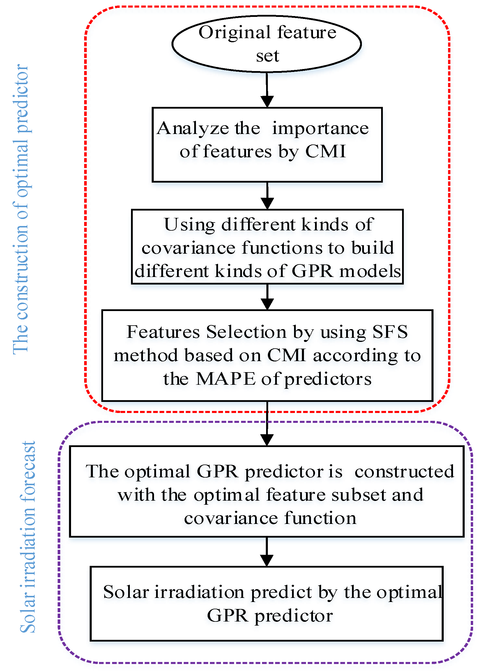
2. Solar Irradiance Forecasting Using CMI and GPR

The new method is mainly composed of two components: CMI and GPR. The purpose of using CMI is to build the optimal feature subset and the optimal predictor is based on the GPR. The combination of the optimal feature subset and the optimal predictor makes up the optimal prediction method.

To build the optimal feature subset, the importance values of different features need to be calculated by CMI first. Then, in terms of the descending order of CMI value, the ranking of feature importance is got. Finally, the feature selection is carried out by using GPR combines the SFS method according to the ranking of feature importance and the optimal feature subset is determined with the minimum error.

To build the predictor of GPR, ten different GPR models with different covariance functions are built. And best covariance function can be selected in the experiment and the optimal predictor is constructed. The optimal predictor method can be determined by the optimal feature subset and optimal predictor. The methodology of the proposed method can be shown in the red box of Figure 1.

When the optimal prediction method is determined, the solar irradiation prediction experiment will be carried out by using this method, as shown in the blue box of Figure 1.

The details about CMI and GPR are explained in the following parts.

2.1. Conditional Mutual Information

CMI makes the new selected features in the subset have strongly correlated with the solar irradiance. It also selects the features with least redundant information.

Suppose that X and Y are two random variables, and $p(x,y)$ is the joint probability distribution of X and Y. The mutual information between X and Y is expressed as:

$$I(X;Y)={\displaystyle \sum _x{\displaystyle \sum _{y}p(x,y)}}\log \frac{p(x,y)}{p(x)p(y)}$$

(1)

When the irradiation value is X, the features to be selected is Y and the selected feature is Z, the CMI is expressed as Y between X and Z:

$$I(X;Y|Z)=I(X;Z)-I(X;Y;Z)$$

(2)

$I(X;Y|Z)$ refers to that the information sharing between X and Y in the case that Z is the selected feature. If Y and Z contains the same amount of information about X, the values of $I(X;Z)$ and $I(X;Y;Z)$ are equal. The value of $I(X;Y|Z)$ is zero. If Y contains information about X but Y does not contain information related to Z, the value of CMI is nonzero. If the X and Y have lower correlation with Z, the amount of shared information $I(X;Y|Z)$ will be bigger and a greater value of CMI will be got. Therefore, CMI takes full account of the information redundancy between candidate features and selected features. That makes the CMI value between the candidate feature and the target feature is the largest. Therefore, it can effectively reduce the redundant information in the optimal feature subset of short term solar irradiation prediction.

2.2. Gauss Process Regression

In the process of feature selection, different feature subsets have different dimension and feature types. It is difficult to ensure the predictor using different feature sets has a well effect with same parameters. Therefore, the predictor with few parameters and stable prediction accuracy will ensure the stability and credibility of feature selection.

Gaussian Process (GP) is a set of any finite number of random variables meet the joint Gauss distribution, which is determined by mean function and covariance function:

$$m(x)=E[f(x)]$$

(3)

$$k(x,x^{\prime })=E[(f(x)-m(x))(f(x^{\prime })-m(x^{\prime }))]$$

(4)

where $x,x^{\prime }\in R^d$ is the arbitrary random variable, $m(x)$ is the expectation of the $f(x)$, $k(x,x^{\prime })$ is the covariance of $x$ and $x^{\prime }$. Therefore, GPR can be defined as $f(x)\sim GP(m(x),k(x,x^{\prime }))$. For the irradiation prediction, using the following model:

$$y=f(x)+\epsilon$$

(5)

$x$ is the input feature vector, $f$ refers to the value of the function, y is the vector of observed value with noise. Assume the noise is $\epsilon ~N(0,{\sigma }_n^2)$, the prior distribution of y can be obtained:

$$y~N(0,K(X,X)+{\sigma }_n^2{I}_n)$$

(6)

The joint prior distribution of the observed value $y$ and the predicted value $f_{*}$ is described as follows.

$$\left[\begin{array}{l}y\\ f_{*}\end{array}\right]~N\left(0,\begin{array}{cc}K(X,X)+{\sigma }_n^2{I}_n& K(X,x_{*})\\ K(x_{*},X)& k(x_{*},x_{*})\end{array}\right)$$

(7)

where $K\left(X,X\right)=K_n=\left(k_{ij}\right)$ is a $n\times n$ symmetric positive definite covariance matrix and the $k_{ij}=k\left(x_i,x_j\right)$ is to measure correlation between feature vector $x_i$ and feature vector $x_j$, $K\left(X,x_{*}\right)=K{\left(x_{*},X\right)}^T$ is the $n\times 1$ covariance matrix between test set $x_{*}$ and the input of training set X. $K\left(x_{*},x_{*}\right)$ is the covariance matrix of test point $x_{*}$. $I_n$ is the n-dimensional unit matrix.

The posterior distribution of the predictive value $f_{*}$ can be calculated by using the following formula:

$$f_{*|X,y,x_{*}}~N({\overline{f}}_{*},\mathrm{cov}(f_{*}))$$

(8)

In this equation,

$${\overline{f}}_{*}=K(x_{*},X){[(X,X)+{\sigma }_n^2{I}_n]}^{-1}y$$

(9)

$$\begin{array}{ll}\mathrm{cov}(f_{*})=\hfill & k(x_{*},x_{*})-K(x_{*},X)\times \\ & {[K(X,X)+{\sigma }_n^2{I}_n]}^{-1}K(X,x_{*})\end{array}$$

(10)

${\widehat{\mu }}_{*}={\overline{f}}_{*}$ and ${\widehat{\sigma }}_{f_{*}}^2=\mathrm{cov}(f_{*})$ are the mean value and variance of the predicted values ($f_{*}$) corresponding to the test points $x_{*}$.

GPR can use different covariance functions. The covariance functions can determine how the response at one point $x_i$ is affected by responses at other points $x_j$, $i\ne j$, $i=1,2,\dots ,n$. The most commonly used covariance function is Squared Exponential Kernel functions:

$$k={\sigma }_f^2\exp [-\frac{1}{2}\frac{{(x_i-x_j)}^T(x_i-x_j)}{{\sigma }_l^2}]$$

(11)

In this equation, ${\sigma }_l$ is the length scale of feature data, ${\sigma }_f$ is the signal standard deviation. The feature length scales briefly define how far apart the input values $x_i$ can be for the response values to become uncorrelated. Both ${\sigma }_l$ and ${\sigma }_f$ need to be greater than 0.

When get the ${\sigma }_l$ and ${\sigma }_f$ is determined, the prediction values $f_{*}$ and variance ${\widehat{\sigma }}_{f_{*}}^2$ can be obtained by using the Equations (9) and (10).

In order to get an accurate prediction value, the decision of GPR need a loss function $L(y,y^{{}_{*}})$, which specifies the loss incurred by predicting the value $y^{*}$ when the true value is $y$. For example, the loss function could equal the absolute deviation between the prediction and the truth. The goal is to make the point prediction $y^{*}$ which incurs the smallest loss. The best prediction, in the sense that it minimizes the expected loss, is:

$$y_{\mathrm{optimal}}=\min {\displaystyle \int L(y,y^{*})}p(y^{*}|x^{*},D)d{y}^{*}$$

(12)

$x^{*}$ is the input data corresponding to $y^{*}$. D is the data set corresponding to $x^{*}$.When the predictive distribution is Gaussian the mean and the median coincide and indeed for any symmetric loss function and symmetric predictive distribution we always get $y$ as the mean of the predictive distribution.

The model is established by GPR applying the principle of probability distribution, then transform the distribution from the prior distribution to the posterior distribution in the Bayesian framework. GPR has less parameters to set. The parameters of GPR can be automatically obtained through the training process and avoid the complex process of parametric optimization. There are less factors affect the prediction stability of GPR [34]. Therefore, its suit for solar irradiation forecast feature selection.

3. Feature Importance and Election Analysis

In this section, part 3.1 is the construction of the feature set. The intuitive analysis of feature sets is carried out in part 3.2. In part 3.3, the further evaluation of feature importance by using CMI, MI and PCC is carried out. In order to select the best feature subset, the sequential forward feature selection is proposed in part 3.4 and part 3.5. In part 3.6, ten kinds of covariance functions of GPR are compered to select the best one. In part 3.7, the feature selection experiments with contrast predictors are carried out and the optimal feature subsets and predictors are determined in this part.

3.1. The Construction of the Data Set

In order to construct the original dataset for the experiment and verify the effectiveness of the method, the measured data collected from SRRL, ORNL and LELH were used respectively. Each data set contains 7 types of meteorological information. In order to accurately identify important features and redundant features among the feature sets, 10 similar neighboring historical features are included in each type of information. At the same time, the Angstrom-Prescott linear regression equation: $\frac{S}{S_0}=a+b\frac{n}{N}$ is usually used to reflect the solar irradiation and the time features [35]. In this equation: S₀ is the extraterrestrial irradiation on horizontal surface (Wh/m²). S is the annual horizontal global solar irradiation (kWh/m²). Coefficients a and b are the empirical coefficients, n is the actual sunshine duration in a day (hours) and N is the monthly average maximum bright sunshine duration in a day (hours). The empirical coefficients a and b depend on the S and n. Considering that the solar irradiation is related to the diurnal and annual variations, the time features are added to the original feature set as date (day) and moment (hour). Therefore, the original feature set is made up of the following features: feature 1 is day, feature 2 is hour; feature 3 to 12 is historical irradiation (S_t-i); feature 13 to 22 is historical temperature (T_t-i); feature 23 to 32 is historical relative humidity (H_t-i); feature 33 to 42 is historical wind direction (Wd_t-i); feature 43 to 52 is historical wind speed (Ws_t-i); feature 53 to 62 is historical air pressure (P_t-i); feature 63 to 72 is historical precipitation (R_t-i), i = 1, 2, ... 10. Among them, t is the time to be predicted; i is the sampling point. Because this work is part of the PV output prediction and according to the requirements of the national grid for short-term and ultra-short-term PV output forecasting, the sampling interval is 15 minutes. The measured data collected from SRRL, ORNL and LELH have the same feature types and data set structure.

3.2. Analysis of Original Feature Set

When using the data from SRRL, the relationship between the meteorological features and solar irradiation can be analyzed by using Figure 2.

The data shown in Figure 2a are randomly selected from 18 February to 24 February 2015. It can be seen from Figure 2a that, the values of solar irradiation, pressure, relative humidity and temperature have obvious daily periodicity. Wind speed, wind direction and precipitation show obvious randomness. In order to show the trend of changes more clearly, the fifth day (in the area of red box) is randomly selected from Figure 2a for detailed analysis. Figure 2b is used to display the data in the red box. Figure 2b is the measured data from 7 to 18 o’clock. At the time of 7 to 12 o’clock, the values of pressure, relative humidity are in the process of decline, while the value of temperature and irradiation are in the process of increase. At the time of 12 to 18 o’clock, the value of pressure and relative humidity are decreased slightly, the value of temperature continues to rise, the values of irradiation began to decline during this time, while the changes of wind speed and wind direction do not show significantly correlated with the solar irradiation.

3.3. Feature Importance Analysis

To analyze the importance of features, three different evaluation methods are used, they are PCC, MI and CMI. In Figure 3, the values of features importance are calculated by CMI, MI and PCC respectively. The measured data are collected from the whole year of 2015 using the data of SRRL. Therefore, the importance values contain the information of the whole year. In order to embody the superiority of CMI in analyzing feature importance and redundancy, the top 12 features are selected and marked in red in Figure 3. As shown in Figure 3, different importance criteria lead to obviously different rankings of feature importance. Compared with PCC and MI, CMI contains more features types (4 types) marked in red in the top 12 features. The features rankings of top 12 according to feature importance are shown in

Table 1. The importance ranking of features of different data sets with different importance analysis method.

Data	Method	Importance Ranking of Features (Top 12)
SRRL	PCC	St-1,St-2,St-3,St-4,St-5,St-6,St-7,St-8,St-9,Tt-1,Ht-1,Tt-2
	MI	St-1,St-2,St-3,hour,St-4,St-5,St-6,St-7,St-8,St-9,St-10,Tt-1
	CMI	St-1,Tt-1,Tt-9,Wst-1,St-6,St-10,Tt-4,St-8,St-5,St-4,St-3,hour
ORNL	PCC	St-1,St-2,St-3,St-4,St-5,St-6,Tt-1,Tt-5,Tt-9,Tt-4,St-7,Wdt-3
	MI	St-1,St-2,St-3,hour,St-4,St-5,St-6,St-7,St-8,St-9,St-10,Tt-1
	CMI	St-1,hour,St-10,St-9,St-8,St-7,Tt-6,St-4,St-3,St-5,St-2,Wst-1
LELH	PCC	St-1,St-2,St-3,St-4,St-5,St-6,St-7,Ht-1,Ht-2,St-8,Ht-3,Ht-4
	MI	St-1,hour,St-2,St-8,St-3,Tt-1,Ht-2,St-5,St-4,St-3,St-2,St-7
	CMI	St-1,St-2,St-3,St-4,Tt-5,Ht-1,St-6,St-8,hour,Ht-4,St-7,Pt-1

and the results of different measured data sets by using different calculation methods can be compared.

Using the data of SRRL as the example to evaluate the ability of different methods about the features correlation and redundancy. As shown in Figure 3 and Table 1, S_t-1 is the most important feature by the 3 methods in SRRL data set. S_t-2 is the most similar feature to the S_t-1, it is behind S_t-1 in the ranking of PCC and MI. But S_t-2 is behind the twelfth at the ranking of CMI importance. Because of the feature sets selected by PCC and MI include many features close in time among the same type, it leads to a large amount of redundancy information contained in the feature sets. The feature set selected by CMI include more features types and has fewer features within the same type. It obviously to see that CMI could evaluate the redundancy of information between features.

In addition, the common features of PCC, MI and CMI in the top 12 features with highest feature importance value include: S_t-1, S_t-3, S_t-4, S_t-5, S_t-6, T_t-1 and so forth. The top 12 features with highest feature importance of the PCC include 3 types of features: historical solar irradiation, temperature and relative humidity. The top 12 features with highest feature importance obtained by MI mainly include 3 types of features: historical irradiation, temperature and time. But the top 12 features with highest feature importance obtained by CMI method include four types of features: historical irradiation, temperature, wind speed and time. Therefore, CMI can fully consider the redundancy between the features in the same type when calculating the feature importance.

Using the same method, the measured data of ORNL and LELH are also used to analyze the importance of features. From Table 1, it can be seen that the ranking of CMI usually contains more type of features than MI and PCC among the top 12 features by the data of ORNL and LELH. So, it can prove that by different data sets, CMI can also effectively analyze the informational redundancy between the features.

At the same time, Table 1 shows that the data sets collected from different locations will have different rankings. Therefore, feature selection needs to be carried out when the different data sets are used.

3.4. Data Description and Evaluation Indicators of Feature Selection

The measured data of SRRL, ORNL and LELH in 2015 are selected as the training set and validation set. Because the values of solar irradiation are greater than zero is mainly concentrated at 7:00 to 19:00, the irradiation values to be predicted are located at this time domain [36].

In this experiment, the validation set is made up of the data four weeks random select from spring, summer, autumn and winter respectively in 2015. Other data is used to constitute training sets. The experiment uses the data with the time interval of 15 minutes. In order to achieve the prediction goal of 1 hour ahead, it needs to do rolling forecast with four steps continuously, the construction of the original feature set and the prediction goal are shown in Figure 4. In Figure 4, the original feature set for feature selection is made up of feature 1 to feature 72, the features marked with t are the original input features of 7 o’clock and the features marked with t’ are the original input features of 19 o’clock. Therefore, S_(t) to S_(t+3) as the 4 prediction values in 7 o’clock and S_(t’) to S_(t’+3) as the 4 prediction values in 19 o’clock. As shown in Figure 4, the dimension of input of the predictor is 72, which increases the complexity of predictor training process and reduces the prediction efficiency. At the same time, there is a lot of redundant information in the original feature set, which makes the prediction accuracy at a lower level. While, feature selection can reduce the dimension of the input features and solve these negative effects.

The feature selection method of SFS is carried out by using MAPE as a measure:

$$MAPE=\frac{1}{m}{\displaystyle \sum _{i=1}^m(|X_t-{\tilde{X}}_t|}/X_t)$$

(13)

where $X_t$ is the real value, ${\tilde{X}}_t$ is the predictive value, m is the number of the predictive value (or real value).

3.5. The Method of Feature Selection Based on CMI and GPR

The SFS process based on CMI and GPR is as follows:

(1) Construct the original feature set;

(2) Using CMI to calculate feature importance;

(3) The SFS method is carried out according to the ranking of features’ importance. GPR predictors is constructed with different feature subsets and the MAPE obtained from the GPR predictor is used as index to determine the optimal features subset.

(4) Finally, the prediction model constructed with the optimal feature subset is used as the final prediction model to predict the solar irradiation.

3.6. Covariance Function Selection and Optimal Predictor Build of GPR

To select the best covariance function of GPR, the experiment of covariance functions selection is proposed. The expressions of 10 covariance functions of GPR are shown in

Table 2. 10 kinds of covariance functions of GPR.

GPR Covariance Function	Mathematical Expression	Function Number
Squared Exponential Kernel	$k(x_i,x_j|\theta )={\sigma }_f^2\exp [-\frac{1}{2}\frac{{(x_i-x_j)}^T(x_i-x_j)}{{\sigma }_l^2}]$	①
Exponential Kernel	$k(x_i,x_j|\theta )={\sigma }_f^2\exp (-\frac{r_1}{{\sigma }_l})$	②
Matern 3/2	$k(x_i,x_j|\theta )={\sigma }_f^2(1+\frac{\sqrt{3}{r}_1}{{\sigma }_l})\exp [-\frac{\sqrt{3}{r}_1}{{\sigma }_l}]$	③
Matern 5/2	$k(x_i,x_j|\theta )={\sigma }_f^2(1+\frac{\sqrt{5}{r}_1}{{\sigma }_l}+\frac{5r_1{}^2}{3{\sigma }_l{}^2})\exp (-\frac{\sqrt{5}{r}_1}{{\sigma }_l})$	④
Rational Quadratic Kernel	$k(x_i,x_j|\theta )={\sigma }_f^2{(1+\frac{r_1{}^2}{2\alpha {\sigma }_l{}^2})}^{-\alpha }$	⑤
ARD Squared Exponential Kernel	$k(x_i,x_j|\theta )={\sigma }_f^2\exp [-\frac{1}{2}{\displaystyle \sum _{m=1}^d\frac{{(x_{im}-x_{jm})}^2}{{\sigma }_m^2}}]$	⑥
ARD Exponential Kernel	$k(x_i,x_j|\theta )={\sigma }_f^2\exp (-r_2)$	⑦
ARD Matern 3/2	$k(x_i,x_j|\theta )={\sigma }_f^2(1+\sqrt{3}{r}_2)\exp (-\sqrt{3}{r}_2)$	⑧
ARD Matern 5/2	$k(x_i,x_j|\theta )={\sigma }_f^2(1+\sqrt{5}{r}_2+\frac{5}{3}{r}_2^2)\exp (-\sqrt{5}{r}_2)$	⑨
ARD Rational Quadratic Kernel	$k(x_i,x_j|\theta )={\sigma }_f^2{(1+\frac{1}{2\alpha }{\displaystyle \sum _{m=1}^d\frac{{(x_{im}-x_{jm})}^2}{{\sigma }_m^2}})}^{-\alpha }$	⑩

[30].

In Table 2, from function ① to ⑤: ${\sigma }_l$ is the feature length scale and the value will not be changed with the input determined. ${\sigma }_f$ is the signal standard deviation. $\theta =[\log {\theta }_l,\log {\theta }_f]$, $r_1=\sqrt{{(x_i-x_j)}^T(x_i-x_j)}$ is the Euclidean distance between $x_i$ and $x_j$. From function ⑥ to ⑩ are the automatic relevance determination covariance function, $r_2=\sqrt{{\displaystyle \sum _{m=1}^d\frac{{(x_{im}-x_{jm})}^2}{{\sigma }_m^2}}}$, where the $d$ is the number of features entered into the predictor, $m=1,\dots ,d$, ${\sigma }_m$ is the feature length scale under the different features, its numeric value will be changed with the different features. ${\sigma }_f$ is the signal standard deviation. $\alpha$ is a parameter which is larger than zero and value of it is determined by ${\sigma }_m$ or ${\sigma }_l$.

10 covariance functions are used to construct 10 GPR models respectively. The training set is used to train the 10 GPR models and the feature selection process is carried out using the validation set in each model. The verification set is constructed by the data randomly selected from the four seasons in 2015. The training set is made up of the remaining data in 2015.

Figure 5 shows the process of feature selection for GPR combines with 10 different covariance functions by using SRRL data sets. Each GPR model combines PCC, MI and CMI to get the error statistics (measured by MAPE). The three methods of PCC-GPR, MI-GPR and CMI-GPR correspond to Figure 5a–c.

It can be seen from Figure 5 that the prediction error decreases with the increase of the feature dimension at first. When the dimension of features from 11 to 40, the error decreases slightly and the predictors with different covariance functions will have a different minimum MAPE value. It can be seen that the accuracy of prediction can be increased by adding redundant features. The black circle in Figure 5 is used to mark the minimum MAPE value. In this process, the value of error is mainly distributed between 10% and 20%. When the dimension of feature set increases to 41 dimensions, all of the error values are greater than the minimum error.

Table 3. Feature selection results with GPR using different covariance functions in different area.

Location	Covariance Function	Predictor
		PCC-GPR		MI-GPR		CMI-GPR
		MAPE min	Feature Dimension	MAPE min	Feature Dimension	MAPE min	Feature Dimension
SRRL	Squared Exponential	10.546	23	10.056	35	9.246	12
	Exponential	10.727	13	10.984	34	9.027	20
	Matern3/2	10.687	29	10.546	36	9.951	18
	Matern5/2	10.469	28	10.479	42	9.096	19
	Rational Quadratic	10.165	29	10.099	40	9.294	21
	ARD Squared Exponential	10.046	34	10.058	35	10.278	17
	ARD Exponential Kernel	9.825	15	9.860	36	8.707	14
	ARD Matern 3/2	10.752	13	9.944	34	10.517	19
	ARD Matern 5/2	10.241	13	10.078	32	8.730	11
	ARD Rational Quadratic	9.932	33	9.957	30	9.396	12
ORNL	Squared Exponential	13.518	40	9.541	36	7.872	18
	Exponential	11.480	41	9.058	34	7.279	23
	Matern3/2	11.871	41	9.481	33	7.130	20
	Matern5/2	11.999	41	9.498	35	7.562	20
	Rational Quadratic	11.253	41	8.456	37	6.862	13
	ARD Squared Exponential	11.130	34	8.284	34	7.025	16
	ARD Exponential Kernel	10.078	33	7.732	32	6.668	16
	ARD Matern 3/2	10.840	36	8.978	32	6.699	20
	ARD Matern 5/2	11.314	46	9.489	30	6.839	24
	ARD Rational Quadratic	10.276	33	8.048	34	7.2726	26
LELH	Squared Exponential	15.581	40	12.792	37	12.180	13
	Exponential	13.869	51	12.479	40	12.548	13
	Matern3/2	14.173	51	12.588	29	13.090	17
	Matern5/2	14.372	51	11.789	30	12.554	23
	Rational Quadratic	12.663	51	11.588	33	12.215	17
	ARD Squared Exponential	12.507	50	11.546	32	11.743	17
	ARD Exponential Kernel	12.386	52	10.843	33	11.806	16
	ARD Matern 3/2	12.941	50	11.548	34	12.011	13
	ARD Matern 5/2	12.840	46	10.954	35	12.303	20
	ARD Rational Quadratic	12.709	42	10.901	32	10.115	16

shows the dimension of optimal feature subset and the minimum MAPE values obtained in the experiment of covariance function selection by using three different data sets of SRRL, ORNL and LELH.

Using the SRRL data, the minimum MAPE of PCC-GPR is 9.825%, the covariance function is ARD Exponential Kernel and the dimension of feature set is 15. The minimum MAPE value of MI-GPR is 9.860%, the covariance function is ARD Exponential Kernel and the feature dimensional is 36. The minimum value of MAPE by CMI-GPR is 8.707%, the covariance function is ARD Exponential Kernel and the feature dimension is 14. The minimum MAPE of CMI-GPR is 1.153% lower than the MAPE of MI-GPR and 2.118% lower than PCC-GPR.

The dimension of optimal feature subset by using CMI-GPR is least, which is 22 less than the dimension of MI-GPR and 1 less than dimension of PCC-GPR. Although the dimension of PCC-GPR’s feature set is 1 more than CMI-GPR, the MAPE value of PCC-GPR is 2.118% larger than CMI-GPR.

In summary ARD Exponential Kernel function shows the best performance of the prediction. So, ARD Exponential Kernel function is selected as the best covariance function of GPR. In the same way, the covariance function selection experiment is performed by using the other two locations: ORNL and LELH.

In comparison, CMI-GPR with ARD-Exponential Kernel (abbreviated as CMI-GPR_AEK) is the optimal predictor when SRRL and ORNL datasets are used. The optimal predictor with its optimal feature subset has better prediction accuracy. When using the LELH dataset, the optimal predictor of CMI-GPR build by ARD Rational Quadratic (abbreviated as CMI-GPR_ARQ) with its optimal feature subset has the better prediction accuracy.

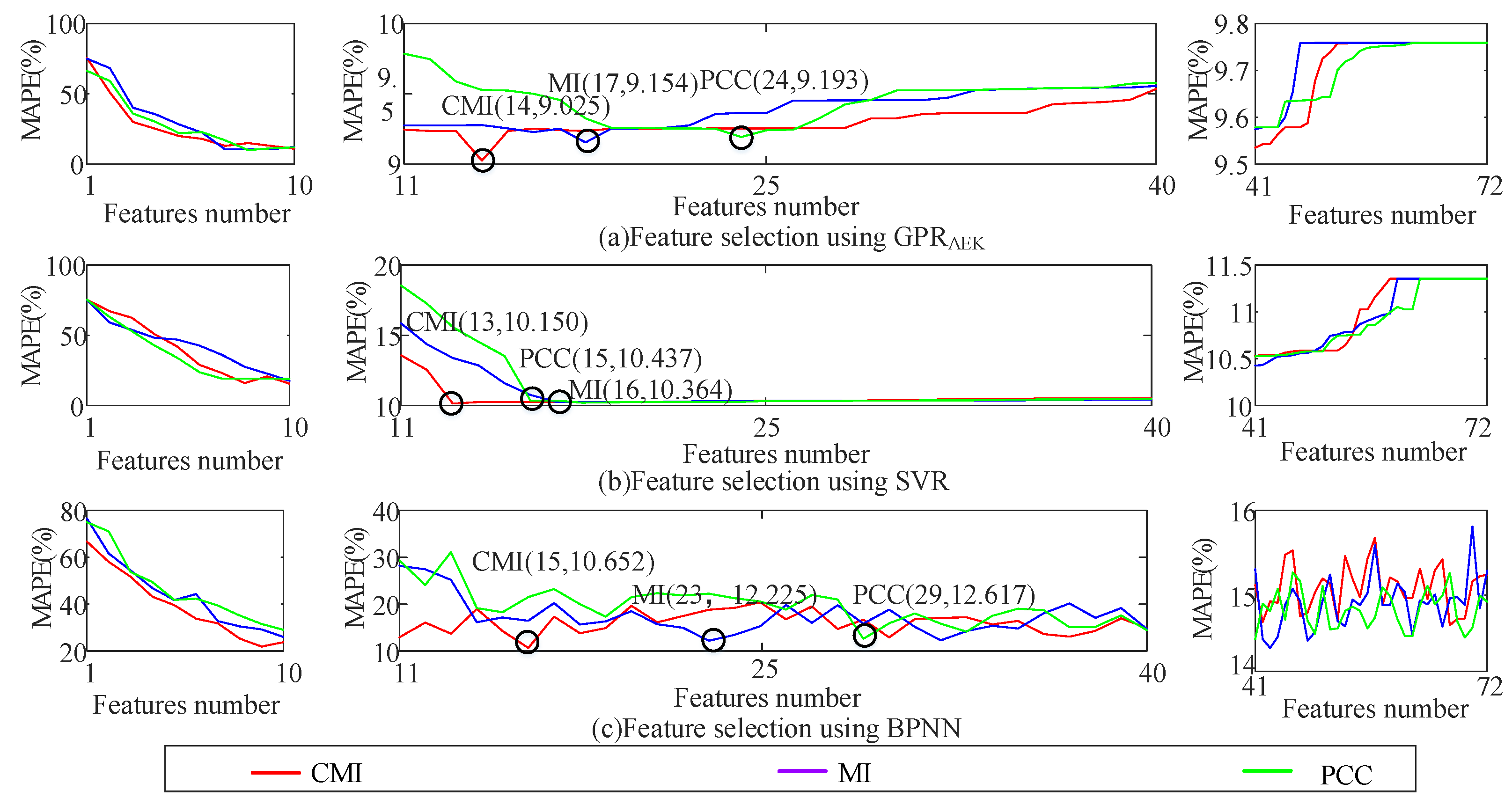
3.7. The Comparison Experiment of Feature Selection

CMI, MI and PCC are combined with BPNN and SVR respectively as the contrastive experiment of the proposed method. The results of feature selection are analyzed in this part. In order to show the difference between different predictors, the same training set and verification set of GPR models were used in the comparison experiment.

In the contrast experiment, the number of input layer and hidden layer nodes of BPNN is set according to Kolmogorov theory: the number of input layer nodes is n₁, the number of hidden layer nodes is n₂. The mathematical relation between n₁ and n₂ is n₂ = n₁ + 1. In the process of feature selection, n₁ and n₂ are adjusted with the changes of the dimension of input features [37,38,39].

The RBF kernel function of is selected as SVR’s kernel function. The cross-validation method is used to determine the parameters of SVR such as the penalty factor c and the variance coefficient g [40]. Then the best combination of parameters is obtained. Setting the [−10,10] to the optimal range of c and g [41,42]. The parameters of GPR, such as the feature length scale ${\sigma }_l$, the signal standard deviation ${\sigma }_f$ and the distributed feature length scale ${\sigma }_m$, can be automatically acquired during training processing according to the dimensions and the length of features [34]. So, the parameter optimization can be simplified.

Figure 6 shows the process of feature selection based on GPR_AEK, SVR and BPNN combined with CMI, MI and PCC respectively using data of SRRL. Figure 6a shows the process of feature selection by GPR_AEK combined with CMI, MI and PCC respectively. When the first 10 features are added to the predictor, predicted error is significantly reduced. Adding new features, the error continuous to reduce and then reaches the minimum MAPE. The value of minimum MAPE is 9.025% and the dimension of feature subset is 14. From the perspective of MAPE, CMI-GPR_AEK obtain the minimum MAPE value (9.025%). The minimum MAPE of MI-GPR_AEK is 9.154%. The smallest MAPE of PCC-GPR_AEK is 9.193%. Therefore, CMI-GPR_AEK has the highest accuracy.

Paying attention to the types and dimension of feature subset, the following conclusions can be obtained: the dimension of the optimal features subset is 14 for CMI-GPR_AEK, the dimension is 17 for MI-GPR_AEK and the dimension is 24 for PCC-GPR_AEK. In the three optimal feature subsets, the CMI-GPR_AEK contains four types of features: historical irradiation, temperature, wind speed and time. MI-GPR_AEK contains four types of features: historical irradiation, moment, temperature and relative humidity. PCC-GPR_AEK contains 3 types of features: historical irradiation, temperature and relative humidity.

Combining the above analysis, the following conclusions can be obtained: the optimal feature subset of CMI-GPR_AEK contains more types of features and has lowest dimension. While the predictor of CMI-GPR_AEK has the highest accuracy than MI-GPR_AEK and PCC-GPR_AEK. Therefore, MI-GPR_AEK and PCC-GPR_AEK contains some redundant and invalid information, which results in lower accuracy and higher dimension of feature subset.

Figure 6b is the processes of feature selection combination of CMI, MI and PCC with SVR. In terms of error, the minimum MAPE is 10.150%, the prediction method is CMI-SVR. In terms of feature’s dimension, the dimension of CMI-SVR is the lowest and the dimension is 13.

As shown in Figure 6c, the feature selection of BPNN with CMI, MI and PCC are obtained. CMI-BPNN has the best results with the minimum MAPE (10.652%) and the dimension of feature subset is 16.

Based on the above analysis, CMI-GPR_AEK, CMI-SVR and CMI-BPNN are the three best predictors after the feature selection by using SRRL data sets.

In order to compare the feature selection with different data sets, the experimental results of ORNL and LELH are sorted out. it is can be seen from

Table 4. Feature selection results in different area.

Data	Predictor	MAPE	Dimension
ORNL	CMI-GPRAKE	6.668	16
	MI-GPRAEK	7.732	20
	PCC-GPRAEK	10.078	25
	CMI-SVR	8.735	14
	MI-SVR	9.738	21
	PCC-SVR	9.962	25
	CMI-BPNN	8.565	16
	MI-BPNN	7.428	23
	PCC-BPNN	9.655	26
LELH	CMI-GPRARQ	10.176	13
	MI-GPRAEK	10.843	23
	PCC-GPRAEK	12.386	25
	CMI-SVR	17.410	14
	MI-SVR	17.956	20
	PCC-SVR	18.732	28
	CMI-BPNN	13.412	24
	MI-BPNN	13.655	28
	PCC-BPNN	14.237	31

that CMI-GPR_AEK and CMI-GPR_ARQ are the optimal predictors when using ORNL and LELH data sets, respectively.

The errors and dimensions of feature subset by using different data sets can be shown in Table 4. The results show that CMI-GPR_AEK and CMI-GPR_ARQ have the highest accuracy and low dimension of the optimal feature subset for different data set.

4. Prediction Experiment of Actual Measured Irradiation Data

In this section, the experiment of solar irradiation prediction is carried out. The optimal feature subsets and optimal predictors are constructed by the experiments of feature selection in chapter 3. The comparative prediction method with different feature selection methods and the basic method with established feature set can be used to testify the validity of the proposed method. The established feature set is built refer to the [43].

4.1. Data Description and The Construction of Predictor with Optimal Subset

In order to demonstrate the universal adaptability and effectiveness of the proposed method in different time, weather conditions and seasons, the measured data of SRRL, ORNL and LELH in 2016 are used to test respectively. The test set is selected from spring, summer, autumn and winter randomly. In the experiment, two covariance functions (ARD Exponential Kernel and ARD Rational Quadratic) are used in GPR to build the optimal GPR predictors (GPR_AEK and GPR_ARQ). Meanwhile, SVR and BPNN as the contrastive predictors.

The construction of optimal features subsets is shown in Table 3 and Table 4. For example, the optimal subsets of CMI-GPR_AEK are composed of the first 14 features in the ranking of feature importance when the SRRL data set is used.

4.2. Valuation Indicators

As for evaluation indicators, Mean Absolute Error (MAE), Relative Mean Absolute Error (rMAE), Root Mean Square Error (RMSE) and Relative Root Mean Square Error (rRMSE) as the indicators to evaluate each method in addition to MAPE [23]. The error formulas are follows:

$$MAE=\frac{{\displaystyle \sum {}_{t=1}^m|X_t-{\widehat{X}}_t|}}{m}$$

(14)

$$rMAE=\frac{{\displaystyle \sum {}_{t=1}^m|X_t-{\widehat{X}}_t|}}{{\displaystyle \sum {}_{t=1}^m{X}_t}}\times 100(\%)$$

(15)

$$RMSE=\sqrt{\frac{{\displaystyle \sum {}_{t=1}^m{(X_t-{\widehat{X}}_t)}^2}}{m}}$$

(16)

$$rRMSE=\frac{RMSE}{\frac{1}{m}{\displaystyle {\sum }_{i=1}^m{X}_t}}\times 100\%$$

(17)

where $X_t$ is the real value, ${\tilde{X}}_t$ is the predictive value, m is the number of the predictive value.

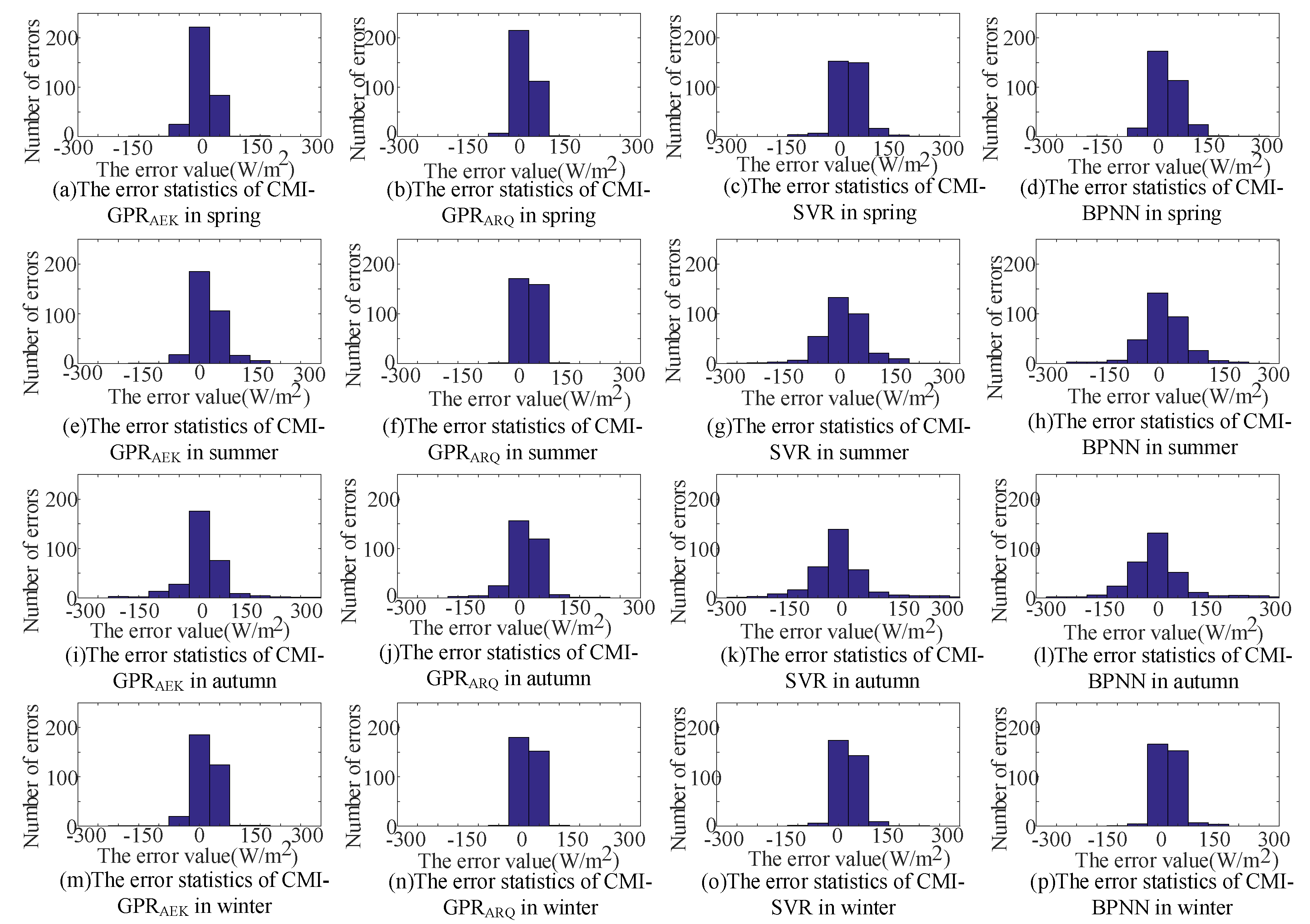
4.3. Prediction Experiment

In order to compare the accuracy of different predictors with their optimal feature subsets, the prediction experiments are carried out in spring, summer, autumn and winter by using the data collected from three locations. When the data of SRRL is used, 4 optimal prediction methods are proposed to verify prediction accuracy, namely, CMI-GPR_AEK, CMI-GPR_ARQ, CMI-SVR and CMI-BPNN. The predicted results are shown in Figure 7 and error statistics are shown in Figure 8. Figure 7 shows the result of solar irradiation forecasting in 4 reasons by 4 different optimal predictors with their optimal feature subset. Figure 8 shows the error distribution of solar irradiation forecasting in 4 reasons by 4 different optimal predictors with their optimal feature subset. As Figure 8 shown, the method has higher predictive accuracy when the absolute value of the error is closer to 0. The result of the errors of different prediction methods (they may not the optimal ones) under the different feature sets are shown in

Table 5. Error statistics of experimental results by SRRL.

Season	Error	Predictor
		CMI-GPRAEK	CMI-GPRARQ	CMI-SVR	CMI-BPNN	MI- GPRAEK	PCC- GPRAEK	MI- GPRARQ	PCC- GPRARQ	GPRAEK	GPRARQ	SVR	BPNN
Spring	MAPE	5.365	5.887	4.776	7.235	6.008	6.245	5.994	7.310	6.987	7.412	10.545	12.461
	RMSE	36.925	78.450	61.080	58.243	62.842	57.472	64.752	69.221	57.158	76.637	89.445	96.575
	MAE	18.387	55.834	43.595	35.807	46.724	39.258	52.100	62.438	40.264	51.942	70.452	75.683
	rRMSE	6.032	9.688	10.432	9.524	9.685	13.759	12.563	13.117	7.002	23.451	18.028	20.076
	rMAE	3.004	6.357	6. 568	5.850	6.421	5.973	7.697	8.082	9.916	6.237	16.47	17.648
Summer	MAPE	8.978	10.537	22.123	16.800	12.824	14.742	14.496	14.059	15.056	15.266	18.481	22.630
	RMSE	40.497	55.041	90.407	118.294	45.630	63.179	59.730	67.872	68.415	72.702	96.014	124.720
	MAE	23.901	31.393	77.140	75.693	29.087	52.476	40.381	57.274	60.174	69.974	78.099	84.269
	rRMSE	8.766	13.185	18.293	28.332	7.925	10.510	16.217	11.033	12.548	12.630	29.239	34.305
	rMAE	4.529	9.519	18.476	16.129	5.693	10.286	10.458	12.131	13.735	14.804	17.642	22.244
Autumn	MAPE	12.184	19.142	25.747	29.458	20.369	23.075	24.259	25.116	30.409	33.547	30.257	32.275
	RMSE	62.950	73.656	98.408	101.067	89.716	90.070	88.646	92.437	89.617	77.908	96.154	135.002
	MAE	26.252	39.790	75.497	86.193	50.435	73.492	48.482	75.668	53.225	51.715	61.390	79.841
	rRMSE	11.307	18.512	24.785	34.456	14.510	18.439	16.803	19.042	18.319	17.865	20.544	35.562
	rMAE	7.838	9.999	18.999	23.671	12.168	17.067	11.374	18.659	12.693	12.374	13.732	18.275
Winter	MAPE	12.472	16.628	16.942	16.992	15.561	17.041	18.418	18.475	17.862	18.300	19.931	22.070
	RMSE	43.921	64.568	81.133	116.209	72.364	75.290	78.821	80.056	77.827	81.273	64.754	98.680
	MAE	25.784	40.487	62.840	78.233	42.640	64.741	62.456	68.671	59.470	61.151	64.754	72.680
	rRMSE	7.384	10.853	15.542	19.524	17.993	18.813	19.003	15.300	13.010	14.726	15.533	17.206
	rMAE	4.325	6.804	9.249	13.820	7.062	14.029	13.998	13.766	11.973	12.266	12.739	14.507
All Year	MAPE	9.750	13.049	17.397	17.621	13.691	15.776	15.792	16.990	17.579	18.631	22.304	18.859
	RMSE	46.073	67.929	82.757	98.453	67.649	71.503	72.987	77.397	73.254	77.130	86.592	113.744
	MAE	23.581	41.877	64.768	68.982	42.222	57.492	50.855	66.0128	53.283	58.700	68.674	78.118
	rRMSE	8.372	13.060	17.263	22.959	12.778	15.380	16.147	14.623	12.720	17.168	20.836	26.787
	rMAE	4.924	8.170	13.323	14.868	7.836	11.839	10.882	13.160	12.079	11.420	15.146	18.169

.

Figure 7a shows the results of a random selected weekly irradiation prediction experiment of spring. As shown in Figure 7a, it is usually sunny in spring and the predictors have a high predictive accuracy. Figure 8a–d show the error distribution of real values and predictive values of solar irradiation in spring, which corresponds to the error distribution of CMI-GPR_AEK, CMI-GPR_ARQ, CMI-SVR and CMI-BPNN respectively. As shown in Figure 8, two of the most precise prediction methods are CMI-GPR_AEK and CMI-GPR_ARQ. Figure 8a shows that the errors are concentrated between −50 W/m² and 50 W/m², while Figure 8c,d show that the distribution of predictive errors about CMI-SVR and CMI-BPNN are relatively dispersed.

As Table 5 shown, the MAPE of CMI-GPR_AEK are the lowest. For other error indicators, such as the rRMSE of CMI-GPR_AEK is decreases about 4.4% and rMAE decreases about 3.564% than CMI-SVR. CMI-GPR_AEK also has shown better predicted accuracy than CMI-GPR_ARQ and CMI-BPNN. CMI-GPR_AEK has the highest predictive accuracy.

Figure 7b shows the results of a random selected weekly irradiation prediction experiment from summer. In Figure 7b, the fluctuation of solar irradiation is undulating in summer, especially in the 2nd, 6th and 7th days. Figure 8e–h shows the error distribution of CMI-GPR_AEK, CMI-GPR_ARQ, CMI-SVR and CMI-BPNN respectively in summer. The number of error’s values between −100 W/m² and 100 W/m² is biggest by using CMI-GPR_AEK. Therefore, the CMI-GPR_AEK has the highest accuracy of prediction. As Table 5 shows, the error value in summer is significantly increased compared with spring. CMI-GPR_AEK predictor has the smallest error. Other error indicators refer to Table 5.

Figure 7c shows the results of a random selected weekly irradiation prediction experiment from autumn. As shown in Figure 7c, the overall trend of autumn is very unstable and the predictive accuracies of the 2nd, 3rd and 5th days is significantly reduced. Figure 8i–l show the error distribution of CMI-GPR_AEK, CMI-GPR_ARQ, CMI-SVR and CMI-BPNN respectively in autumn. The predictor of CMI-GPR_AEK is the best. Compared with CMI-GPR_AEK, the error of CMI-GPR_ARQ increased by 6.958% in MAPE, increased by 7.205% in rRMSE and 2.161% in rMAE. The predictive errors of CMI-SVR and CMI-BPNN are obviously worse than CMI-GPR_AEK and CMI-GPR_ARQ.

Figure 7d shows the results of a random selected weekly irradiation prediction experiment from winter. As shown in Figure 7d, the 2nd and 4th days of real value fluctuates obviously in winter while the other five days of real value are less volatile. Figure 8m–p shows the distribution of error by using MI-GPR_AEK, CMI-GPR_ARQ, CMI-SVR and CMI-BPNN in winter and CMI-GPR_AEK has the best distribution of error. As the Table 5 shows, the MAPE of CMI-GPR_AEK is 12.472%. Other predictors: the MAPE values of CMI-GPR_ARQ, CMI-SVR and CMI-BPNN are 16.628%, 16.942% and 16.992% respectively.

From the errors of all year to analyze the result of prediction, CMI-GPR_AEK has the highest predictive accuracy. The MAPE of CMI-GPR_AEK is 5.365%. It is decreased about 3.299% than CMI-GPR_ARQ, 7.647% than CMI-SVR and 7.871% than CMI-BPNN. As shown in Table 5, by using other indexes of error evaluation, the CMI-GPR_AEK also shows the best performance.

To verify the effectiveness of the proposed method, the statistical errors about suboptimal prediction method are shown in Table 5. From Table 5, it can be seen that, the methods by using PCC and MI have higher errors than by using CMI generally. For example, in spring, the RMSE of CMI-GPR_AEK is 25.917 W/m² lower than MI-GPR_AEK and 20.547 W/m² lower than PCC-GPR_AEK. In summer, the MAPE of MI-GPR_AEK and PCC-GPR_AEK is 3.846% and 5.764% higher than CMI-GPR_AEK.

When compare the results of the basic methods and the proposed methods, it can be found that the errors of basic method by using established feature sets is generally higher than proposed method. For example, the MAPE of GPR_AEK is 1.662% higher than CMI-GPR_AEK in spring and 6.078% higher in summer. The other details of error data are shown in Table 5.

Therefore, CMI-GPR_AEK can be considered the best prediction method in solar irradiation prediction by using the data of SRRL.

To testify the adaptability of the proposed method, the verification experiments of solar irradiation are carried out by using the data of ORNL and LELH at the same time. In the verification experiments, GPR_AEK shows the higher accuracy than SVR, BPNN and GPR_ARQ. To make further compare the influence of different feature subsets on the solar irradiation prediction, the error statistics of GPR_AEK combines CMI, MI and PCC (named as CMI-GPR_AEK, MI-GPR_AEK and PCC-GPR_AEK respectively) and the GPR_AEK combines the constructed feature set (named as GPR_AEK) are shown respectively in

Table 6. Error statistics of experimental results by ORNL and LELH.

Season	Error	Predictor
		CMI-GPRAEK		MI-GPRAEK		PCC-GPRAEK		GPRAEK
		ORNL	LELH	ORNL	LELH	ORNL	LELH	ORNL	LELH
Spring	MAPE	12.472	7.204	14.151	8.410	16.277	8.203	16.832	9.242
	RMSE	43.925	24.491	54.581	37.423	49.488	42.996	51.755	48.666
	MAE	25.786	20.036	34.574	33.824	26.154	30.674	30.287	29.825
	rRMSE	7.387	5.968	11.586	6.652	11.262	6.746	12.131	7.023
	rMAE	4.321	4.122	9.478	8.776	6.469	6.409	7.247	6.371
Summer	MAPE	12.183	9.595	15.616	10.867	16.458	10.020	16.026	10.547
	RMSE	62.954	23.357	71.623	25.023	72.090	25.176	70.249	26.739
	MAE	26.256	9.209	34.472	18.135	36.534	16.694	37.012	18.274
	rRMSE	11.305	3.280	13.767	5.516	17.902	5.552	16.866	5.951
	rMAE	7.839	2.251	6.798	5.627	9.514	7.475	9.335	7.923
Autumn	MAPE	5.367	9.192	6.319	10.809	7.282	9.762	7.873	10.686
	RMSE	36.924	34.457	47.640	45.290	49.051	37.621	55.525	42.684
	MAE	18.383	19.085	29.716	26.008	32.112	26.725	35.647	30.007
	rRMSE	6.031	5.457	7.014	6.473	6.384	6.636	6.561	7.012
	rMAE	3.004	3.162	6.312	4.204	7.275	6.279	7.144	7.034
Winter	MAPE	8.974	6.622	11.845	8.971	10.497	9.322	11.709	9.297
	RMSE	40.497	21.305	54.428	26.435	49.569	30.111	56.688	29.725
	MAE	23.900	8.487	32.379	15.094	29.630	17.263	31.120	17.242
	rRMSE	8.762	4.878	10.002	5.002	9.833	6.265	11.196	6.241
	rMAE	4.523	3.654	6.725	4.204	5.742	7.537	6.915	7.638
All Year	MAPE	9.749	8.153	11.983	9.764	12.629	9.327	13.110	9.943
	RMSE	46.075	25.903	57.068	33.543	55.050	33.976	58.554	36.954
	MAE	23.581	14.204	32.785	23.265	31.108	22.839	33.517	23.837
	rRMSE	8.371	4.896	10.592	5.911	11.345	6.300	11.689	6.557
	rMAE	4.922	3.297	7.328	5.703	7.250	6.925	7.660	7.242

.

As shown in Table 6, using the data of ORNL and LELH, CMI-GPR_AEK shows the lower errors than the other prediction methods. For example, when using the data of ORNL, the rRMSE of CMI-GPR_AEK is 3.302% than GPR_AEK, is 2.221% lower than MI-GPR_AEK and is 2.983% lower than PCC-GPR_AEK. Therefore, CMI-GPR_AEK is the best prediction method with the highest predictive accuracy.

Comprehensive consideration of irradiation prediction experiments using 3 different data sets, CMI-GPR_AEK has higher predictive accuracy. Therefore, the best prediction method is CMI-GPR_AEK.

5. Conclusions

In order to determine the optimal feature subset of solar irradiation prediction and construct the optimal predictor, the new feature selection method of the irradiation prediction based on CMI and GPR is proposed. This method can avoid the negative effects of redundancy between features in the feature subset and improve the forecast accuracy by the GPR with ARD Exponential Kernel function.

The following results are obtained:

(1) When the importance of features is analyzed by CMI, the optimal feature subset with low redundancy of information and strong correlation between the selected features are constructed. Therefore, the influence of redundancy in the irradiation prediction can be reduced.

(2) From the experiment of solar irradiation forecasting, GPR shows the higher prediction accuracy. It could determine the parameters automatically and avoid the complex parameters optimization process, which is the advantage for feature selection.

(3) The predict ability of GPR with different covariance functions has been analyzed and the covariance function of ARD Exponential Kernel is chosen to construct the predictor according to the experiment results. CMI-GPR_AKE is the best prediction model with low feature dimension and the highest prediction accuracy. The dimension of optimal feature set of CMI-GPR_AKE is 14, which is 5 lower than PCC-GPR_AKE and 11 lower than MI-GPR_AEK. The MAPE of solar irradiation forecasting of CMI-GPR_AEK is 3.299% lower than CMI-GPR_ARQ, 7.647% lower than CMI-SVR and 7.871% lower than CMI-BPNN.

References

1. Arash, A.; Wu, T.X.; Ramos, B. A Hybrid Algorithm for Short-Term Solar Power Prediction—Sunshine State Case Study. IEEE Trans. Sustain. Energy 2017, 8, 582–591. [Google Scholar]
2. Emre, A.; Hocaoglu, F.O. A Novel Method Based on Similarity for Hourly Solar Irradiance Forecasting. Renew. Energy 2017, 112, 337–346. [Google Scholar]
3. Fidan, M.; Hocaoğlu, F.O.; Gerek, Ö.N. Harmonic analysis based hourly solar radiation forecasting model. IET Renew. Power Gen. 2015, 9, 218–227. [Google Scholar] [CrossRef]
4. Jamil, B.; Akhtar, N. Comparative analysis of diffuse solar radiation models based on sky-clearness index and sunshine period for humid-subtropical climatic region of India: A case study. Renew. Sustain. Energy Rev. 2017, 78, 329–355. [Google Scholar] [CrossRef]
5. Emanuele, O. Physical and hybrid methods comparison for the day ahead PV output power forecast. Renew. Energy 2017, 113, 11–21. [Google Scholar] [Green Version]
6. Ayush, S. Solar Irradiance Forecasting in Remote Microgrids using Markov Switching Model. IEEE Trans. Sustain. Energy 2016, 99, 1. [Google Scholar]
7. Inanlouganji, A.; Reddy, T.A.; Katipamula, S. Evaluation of regression and neural network models for solar forecasting over different short-term horizons. Sci. Technol. Built Environ. 2018, 24, 12–22. [Google Scholar] [CrossRef]
8. Tingting, Z. Clear-sky model for wavelet forecast of direct normal irradiance. Renew. Energy 2017, 104, 1–8. [Google Scholar]
9. Shahaboddin, S. A comparative evaluation for identifying the suitability of extreme learning machine to predict horizontal global solar radiation. Renew. Sustain. Energy Rev. 2015, 52, 1031–1042. [Google Scholar]
10. Tao, H. A Practical Method to Hourly Forecast the Solar Irradiance. Presented at 3rd International Conference on Material, Mechanical and Manufacturing Engineering (IC3ME 2015), Guangzhou, China, 27–28 June 2015. [Google Scholar]
11. Stéphanie, M. Hourly forecasting of global solar radiation based on multiscale decomposition methods: A hybrid approach. Energy 2017, 119, 288–298. [Google Scholar]
12. Inman, R.H.; Pedro, H.T.C.; Coimbra, C.F.M. Solar forecasting methods for renewable energy integration. Prog. Energy Combust. Sci. 2013, 39, 535–576. [Google Scholar] [CrossRef]
13. Bigdeli, N.; Borujeni, M.S.; Afshar, K. Time series analysis and short-term forecasting of solar irradiation, a new hybrid approach. Swarm Evol. Comput. 2016. [Google Scholar] [CrossRef]
14. Reikard, G.; Haupt, S.E.; Jensen, T. Forecasting ground-level irradiance over short horizons: Time series, meteorological and time-varying models. Renew. Energy 2017. [Google Scholar] [CrossRef]
15. Bracale, A.; Carpinelli, G.; De Falco, P. A Probabilistic Competitive Ensemble Method for Short-Term Photovoltaic Power Forecasting. IEEE Trans. Sustain. Energy 2016, 99, 1. [Google Scholar] [CrossRef]
16. Fatih Onur, H.; Serttas, F. A novel hybrid (Mycielski-Markov) model for hourly solar radiation forecasting. Renew. Energy 2016, 108, 635–643. [Google Scholar]
17. Michael, K.; Kluge, J. A new hybrid support vector machine–wavelet transform approach for estimation of horizontal global solar radiation. Energy Convers. Manag. 2015, 92, 162–171. [Google Scholar]
18. Amit Kumar, D. A new hybrid feature selection approach using feature association map for supervised and unsupervised classification. Expert Syst. Appl. 2017, 88, 81–94. [Google Scholar]
19. Leily, S.; Alizadeh, S.H. A note on pearson correlation coefficient as a metric of similarity in recommender system. In Proceedings of the AI & Robotics, Qazvin, Iran, 12 April 2015; pp. 1–6. [Google Scholar]
20. Jianzhou, W. Forecasting solar radiation using an optimized hybrid model by Cuckoo Search algorithm. Energy 2015, 81, 627–644. [Google Scholar]
21. Li, S.; Ping, W.; Goel, L. Wind Power Forecasting Using Neural Network Ensembles With Feature Selection. IEEE Trans. Sustain. Energy 2017, 6, 1447–1456. [Google Scholar] [CrossRef]
22. Haomiao, Z. A new sampling method in particle filter based on Pearson correlation coefficient. Neurocomputing 2016, 216, 208–215. [Google Scholar]
23. Manzano, A. A single method to estimate the daily global solar radiation from monthly data. Atmos. Res. 2015, 166, 70–82. [Google Scholar] [CrossRef]
24. Xinguang, H.; Guan, H.; Qin, J. A hybrid wavelet neural network model with mutual information and particle swarm optimization for forecasting monthly rainfall. J. Hydrol. 2015, 527, 88–100. [Google Scholar]
25. Estevez, P.A.; Tesmer, M.; Perez, C.A.; Zurada, J.M. Normalized mutual information feature selection. IEEE Trans. Neural Netw. 2009, 20, 189–201. [Google Scholar] [CrossRef] [PubMed]
26. François, F. Fast Binary Feature Selection with Conditional Mutual Information. J. Mach. Learn. Res. 2003, 5, 1531–1555. [Google Scholar]
27. Abderrezak, L.; Mordjaoui, M.; Dib, D. One-hour ahead electric load and wind-solar power generation forecasting using artificial neural network. In Proceedings of the Sixth International Renewable Energy Congress, Sousse, Tunisia, 24–26 March 2015; pp. 1–6. [Google Scholar]
28. Che, J.; Yang, Y.; Li, L.; Bai, X.; Zhang, S.; Deng, C. Maximum relevance minimum common redundancy feature selection for nonlinear data. Inf. Sci. 2017, 409–410, 68–86. [Google Scholar]
29. Chao, H.; Zhang, Z.; Bensoussan, A. Forecasting of daily global solar radiation using wavelet transform-coupled Gaussian process regression: Case study in Spain. In Proceedings of the Innovative Smart Grid Technologies—Asia (ISGT-Asia), Sousse, Tunisia, 28 Novemver–1 December 2016; pp. 799–804. [Google Scholar]
30. Zhang, C. A Gaussian process regression based hybrid approach for short-term wind speed prediction. Energy Convers. Manag. 2016, 126, 1084–1092. [Google Scholar] [CrossRef]
31. NREL Website. Available online: http://midcdmz.nrel.gov/nelha/ (accessed on 9 August 2018).
32. ORNL Website. Available online: http://midcdmz.nrel.gov/ornl_rsr/ (accessed on 9 August 2018).
33. NELHA Website. Available online: http://midcdmz.nrel.gov/nelha/ (accessed on 9 August 2018).
34. Rasmussen, C.E.; Nickisch, H. Gaussian Processes for Machine Learning (GPML) Toolbox. J. Mach. Learn. Res. 2010, 11, 3011–3015. [Google Scholar]
35. Li, D.; Lam, T.; Chu, C. Relationship between the total solar radiation on tilted surfaces and the sunshine hours in Hong Kong. Sol. Energy 2008, 82, 1220–1228. [Google Scholar] [CrossRef]
36. Gagn, D.J., II; McGovern, A.; Haupt, S.E.; Williams, J.K. Evaluation of statistical learning configurations for gridded solar irradiance forecasting. Sol. Energy 2017, 150, 383–393. [Google Scholar] [CrossRef]
37. Zhao, E.F.; Jin, Y. Dam Deformation Monitoring Model and Forecast Based on Hierarchical Diagonal Neural Network. In Proceedings of the 2008 4th International Conference on Wireless Communications, Networking and Mobile Computing, Dalian, China, 12–14 October 2008; pp. 1–4. [Google Scholar]
38. Maniezzo, V. Genetic evolution of the topology and weight distribution of neural networks. Neural Netw. IEEE Trans. 1994, 5, 39–53. [Google Scholar] [CrossRef] [PubMed]
39. Cervone, G. Short-term photovoltaic power forecasting using Artificial Neural Networks and an Analog Ensemble. Renew. Energy 2017, 108, 274–286. [Google Scholar] [CrossRef]
40. Jiang, H. A short-term and high-resolution distribution system load forecasting approach using support vector regression with hybrid parameters optimization. IEEE Trans. Smart Grid. 2017, 99, 1. [Google Scholar] [CrossRef]
41. He, J.; Yao, D. A nonlinear support vector machine model with hard penalty function based on glowworm swarm optimization for forecasting daily global solar radiation. Energy Conv. Manag. 2016, 126, 991–1002. [Google Scholar]
42. Belaid, S.; Mellit, A. Prediction of daily and mean monthly global solar radiation using support vector machine in an arid climate. Energy Conv. Manag. 2016, 118, 105–118. [Google Scholar] [CrossRef]
43. He, J.; Yao, D. Forecast of hourly global horizontal irradiance based on structured Kernel Support Vector Machine: A case study of Tibet area in China. Energy Conv. Manag. 2017, 142, 307–321. [Google Scholar]
Figure 1. The flowchart of the proposed method.
Sustainability 10 02889 g001
Figure 2. The relationship between different meteorological features and solar irradiation. (a) The original data for a week in September 2015 (b) Enlarge the data in the red box.
Sustainability 10 02889 g002
Figure 3. The importance of features using different importance analysis method.
Sustainability 10 02889 g003
Figure 4. The description of original feature set and prediction goal.
Sustainability 10 02889 g004
Figure 5. Feature selection process with different GPR covariance functions.
Sustainability 10 02889 g005
Figure 6. The process of feature selection with different predictors and different importance analysis methods.
Sustainability 10 02889 g006
Figure 7. The result of solar irradiation forecasting with different predictors using optimal feature subset.
Sustainability 10 02889 g007
Figure 8. The histogram of the error by different predictor in 4 seasons using the optimal feature subset.
Sustainability 10 02889 g008