Does the Complexity of Evapotranspiration and Hydrological Models Enhance Robustness?

Abstract

In this study, five hydrological models of increasing complexity and 12 Potential Evapotranspiration (PET) estimation methods of different data requirements were applied in order to assess their effect on model performance, optimized parameters, and robustness. The models were applied over a set of 10 catchments that are located in South Korea. The Shuffled Complex Evolution-University of Arizona (SCE-UA) algorithm was implemented to calibrate the hydrological models for each PET input while considering similar objective functions. The hydrological models’ performance was satisfactory for each PET input in the calibration and validation periods for all of the tested catchments. The five hydrological models’ performance were found to be insensitive to the 12 PET inputs because of the SCE-UA algorithm’s efficiency in optimizing model parameters. However, the five hydrological models’ parameters in charge of transforming the PET to actual evapotranspiration were sensitive and significantly affected by the PET complexity. The values of the three statistical indicators also agreed with the computed model evaluation index values. Similarly, identical behavioral similarities and Dimensionless Bias were observed in all of the tested catchments. For the five hydrological models, lack of robustness and higher Dimensionless Bias were seen for high and low flow as well as for the Hamon PET input. The results indicated that the complexity of the hydrological models’ structure and the PET estimation methods did not necessarily enhance model performance and robustness. The model performance and robustness were found to be mainly dependent on extreme hydrological conditions, including high and low flow, rather than complexity; the simplest hydrological model and PET estimation method could perform better if reliable hydro-meteorological datasets are applied.

1. Introduction

Hydrological models are used to predict low flows, floods, and groundwater recharge, and to develop safe and sustainable water resource strategies [1]. As a result, understanding the water resources systems and reliable information play a vital role to achieve environmentally sound and sustainable water management [2,3,4]. Moreover, Horne [5] addressed the importance of upgrading water information systems (data series) to enhance sustainable water management. Similar findings were made by Chung et al. [6] in a study of robust water resource vulnerability assessment in a Korean watershed. However, the model output should be reliable and robust for applications in an operational context [7]. Perrin et al. [7] defined the term robustness of a model as “the ability to perform under as varied a set of hydrological conditions as possible”, and the same definition is used hereafter. The benefits and limitations of using a parsimonious model over an inadequate complexity were discussed by Perrin et al. [7], and in a similar study, the authors addressed model over-parameterization and parameter uncertainty problems of an inadequate complexity. The term complexity hereafter refers to “the number of parameters optimized during the calibration phase” [7] for the hydrological models and data requirements for the PET estimation methods. Identifying the appropriate hydrological model structure and their corresponding climate input is crucial in reducing hydrological model uncertainty [8]. Several hydrological models have been developed in the past few decades with different assumptions on the rainfall-runoff process and data requirements. Due to the complex nature of the hydrological systems, each hydrologist might not necessarily agree with the rainfall-runoff process, but there exist general themes in common, which agree about the dominant hydrological processes [9].

Although physically-based and spatially-distributed models have the ability to represent internal physical processes, parameter estimation can be challenging due to a problem of sub-grid scale processes [10,11,12,13]. In contrast, conceptual rainfall-runoff models are parsimonious and they perform well when calibrated against measured runoff data [14,15,16]. Furthermore, several studies have shown the applicability of conceptual rainfall-runoff models in different spatial and temporal scales using basic climate datasets and simple Potential Evapotranspiration (PET) estimation methods [17,18,19,20]. Evapotranspiration is an essential component of the hydrological cycle, especially in semiarid and arid regions [21], and it exceeds runoff in 77% of the global land surface [22]. It is often difficult to decide which PET estimation method to use for a particular purpose because of the differences in their approach and data requirements. However, understanding the dominant physical processes and factors affecting PET estimation is crucial for rainfall-runoff modelling, catchment, and reservoir management applications [23].

A study conducted to test the sensitivity of hydrologic models to random fluctuations and constant biases in PET inputs leaving other inputs and parameters unaffected showed a significant error in simulated peak flow and recession characteristics due to the introduced constant bias [24]. However, other model sensitivity analyses studies that were conducted in diverse catchments indicated that precipitation data errors produced more uncertainties on model output than PET data errors [25,26,27,28]. Although selecting the most relevant PET estimation methods for catchment modelling is challenging, researchers have often recommended the Penman-Monteith method as the standard for reference evaporation estimation, which is a physically-based combination equation that is able to describe the evaporation processes [29,30]. A study conducted to analyze the sensitivity of the Hydrologiska Byråns Vattenbalansavdelning (HBV) model using seven PET inputs showed that the Penman PET input had a slightly better model performance than other PET estimation methods [31] and similar results were also observed in another study [32].

Doubts on selecting complex or simple PET estimation methods for rainfall–runoff modelling were raised by Morton [33]. Evans [34] showed the potential of using direct precipitation and temperature input data instead of PET for better streamflow predictions after testing the Catchment Moisture Deficit-Identification of unit Hydrographs and Component flows from Rainfall, Evaporation and Streamflow data (CMD-IHACRES) model while considering four regional climate models (RCMs) in the central United States. Furthermore, the capability of the Génie Rural à 4 paramètres Journalier (GR4J) and the TOPography based hydrological MODEL (TOPMODEL) to overcome systematic errors was presented by testing a sample of 62 catchments in the central mountainous region of France [17]. Andréassian et al. [17] applied a simple and a more accurate PET input obtained from regionalization and the result showed similar model performance due to the ability of the model parameters to adapt to various PET inputs during the calibration. A similar finding was obtained by applying a similar model using 27 PET inputs for a sample of 308 catchments that are located in France, the United States, and Australia [35,36]. Furthermore, two additional lumped rainfall-runoff were tested using similar datasets and catchments [19,20] and Oudin et al. [20] suggested the use of temperature-based PET estimation methods after considering its simplicity and efficiency.

The Nash and Sutcliffe [37] index value is commonly used in evaluating hydrological model performance. However, the Nash-Sutcliffe Efficiency (NSE) has been criticized in recent studies due to its oversensitivity to extreme values [38,39]. In addition, the minor differences in the NSE index value makes it difficult to compare hydrological model structures of different complexity. Moriasi et al. [40] recommended the use of the NSE, and the ratio of the root mean square error to the standard deviation of measured data (RSR) to evaluate hydrological model performances for streamflow simulation. The logarithm transformed NSE (LogNSE) performance measure is often used in order to put more weight on lowflow simulation. Moussa and Chahinian [39] advised considering various objective functions besides the widely used NSE efficiency measure. Gupta et al. [41] proposed the Kling-Gupta Efficiency (KGE), which considered different components, including correlation, variance, and mean for evaluating hydrological models. Jung et al. [16] also addressed the benefit of considering a multiobjective function for calibrating a hydrological model. In this study, four objective functions were considered: the NSE, Log NSE, KGE, and RSR (which is related the Root Mean Square Error (RMSE)) to calibrate five hydrologic models for each PET input.

Clark et al. [42] presented the challenges of identifying the most appropriate model’s structure in the discipline of hydrology and developed the Framework for Understanding Structural Errors (FUSE). The Akaike Information Criterion (AIC) proposed by Akaike [43] and the Bayesian Information Criterion (BIC) suggested by Schwarz [44] are commonly applied model comparison criteria used to select the most appropriate model structure. The Adjusted R-square (Ra²) statistical indicator is also often used as an alternative criterion for comparing different model structures [39]. The AIC basically assumes the Kullback-Leibler’s information and the BIC uses Bayesian approaches to estimate the variations between the observed and simulated models. The AIC, BIC, and Ra² statistical indicators are able to balance performance against model complexity (the number of parameters). After the computation of the statistical indicators, the model with a minimum value of AIC, BIC, and the maximum value of Ra² can be adopted for practical application [45,46].

Robustness is an essential quality of any model, but hydrological models often tend to perform differently between calibration and validation periods [7]. Other studies have also argued the importance of minimizing the water balance errors in the model calibration process to enhance hydrological model robustness [47,48]. Coron et al. [48] suggested comparing the Dimensionless Bias (the ratio of 10 year mean simulated and observed flows) to investigate the robustness and tested the method while using three hydrological models of increasing complexity over 20 French catchments. The Dimensionless Bias must be one for a perfectly robust model. In this study, three statistical indicators (AIC, BIC, and Ra²) were used to select the most appropriate model structure among the applied five hydrological models of increasing complexity and 12 PET estimation methods. Similarly, the model robustness was evaluated by comparing the Dimensionless Bias of five hydrological models for 12 PET inputs.

The main objective of this study was to assess the effects of five hydrological models of increasing complexity and 12 PET estimation methods of different data requirements on model performance, optimized parameters, and robustness. Specifically, three research questions were addressed: (i) does the complexity of hydrological models enhance model performance? (ii); does the complexity of PET estimation methods have analogous effects on optimized parameters?; and, (iii) does increasing the complexity of PET estimation methods and hydrological models enhance robustness? We applied five hydrological models: GR4J, Simplified HYDROLOG (SIMHYD), Catchment Hydrological Cycle Assessment Tool (CAT), TANK, and Sacramento Soil Moisture Accounting (SAC-SMA) models that considered the combined, radiation, and temperature-based PET estimation methods in a sample of 10 catchments that are located in South Korea (8.5–6648 km²). The five hydrological models and 12 PET estimation methods had different levels of complexity. The GR4J (four parameters), SIMHYD (seven parameters), CAT (eight parameters), TANK (12 parameters), and SAC-SMA (16 parameters) models were selected when considering their wide applications in several basins. Similarly, the 12 PET estimation methods required different climatic variables including mean Temperature (T), Wind Speed (u), Relative Humidity (RH), and Solar Radiation (R_S) data depending on the level of complexity. The available hydro-meteorological data obtained from 10 catchments were used to set up and calibrate five hydrological models for 12 PET inputs. The Thiessen polygon method was used for estimating the mean areal precipitation. There exist several kinds of optimization methods for calibrating hydrological models and the Shuffled Complex Evolution-University of Arizona (SCE-UA) algorithm is often adopted by researchers due to its broad applications, efficiency, and robustness [49,50,51,52]. In this study, the SCE-UA algorithm was used to optimize the hydrological model parameters for each PET input by setting a similar objective function: NSE, LogNSE, KGE, and RSR. The detailed description of the 10 catchments hydrological characteristics, the dataset used, the methodology adopted, the result, and discussions are presented in the next sections.

2. Materials and Methods

2.1. Study Area

In this study, 10 catchments were selected, which are based on the availability of continuous streamflow data from different climate zones in South Korea. The selected catchments represent the major hydrological characteristics of the Korean Peninsula with fewer anthropogenic effects on flow over the modelling period. The catchments are located in unregulated and mountainous regions and the catchment areas vary from 8.5 to 6648 km². The main hydrological characteristics of the catchments are concentrated in summer (June to September), contributing to 70% of the precipitation that leads to peak flow. However, the snowmelt effect is not significant in these regions due to the limited amount of winter precipitation (December to February). The location of the 10 catchments, major rivers, and streamflow gauging stations are shown in Figure 1.

2.2. Data

The dataset that is used in this study consisted of daily hydro-meteorological measurements with no missing records over the application period (2001–2012) for nine gauged catchments. However, for the Kyeongan catchment, the available observed streamflow data (1999–2008) were used. The observed streamflow data at the outlet of the catchment and the areal precipitation data generated using the Thiessen polygon method were acquired from the Water Resources Management Information System operated by the Ministry of Land, Infrastructure, and Transport of the Korean Government. The climate data used for estimating PET were provided by the Korea Meteorological Administration. The hydro-meteorological data used for the Seolmacheon experimental catchment are managed by the Korea Institute of Civil Engineering and Building Technology (KICT). The climate data obtained from each station to estimate PET include daily T (°C), RH (%), u (m/s), and R_S (MJ/m² d) estimated from the daily sunshine hours (n) while using the Ångström-Prescott equation [53]. The major hydrological characteristics and hydro-climate conditions of the catchments are summarized in

Table 1. Hydrological characteristics of the 10 gauged catchments.

No	1 Catchment	Area (km2)	Mean Annual T (°C)	Mean Annual P (mm)	Mean Annual PET (mm)	Mean Annual Q (mm)	PET/P	Q/P
1	Seolmacheon	8.50	11.19	1542.30	1226.65	1064.40	0.80	0.69
2	Boryeong	163.70	12.77	1425.43	1012.27	882.52	0.71	0.62
3	Kyeongan	262.40	12.76	1400.28	1326.09	937.12	0.95	0.67
4	Seomjingang	763	11.91	1466.98	815.19	883.34	0.56	0.60
5	Yongdam	930	11.11	1477.57	883.27	904.69	0.60	0.61
6	Juam	1010	14.61	1595.86	1017.39	776.18	0.64	0.49
7	Imha	1361	12.52	1073.55	940.98	575.06	0.88	0.54
8	Andong	1584	11.82	1302.23	1032.93	728.20	0.79	0.56
9	Soyanggang	2703	11.78	1394.90	840.89	915.85	0.60	0.66
10	Chungju	6648	12.10	1406.93	922.96	930.96	0.66	0.66

¹ The analysis period (2002–2012) was the same for all catchments except Kyeongan (2000–2008). Mean Temperature (T), Potential Evapotranspiration (PET), Precipitation (P), and Streamflow (Q).

. The mean annual PET was estimated using the Penman-Monteith method.

The input data for the physically based hydrological model (CAT) were extracted from land use and soil data provided by the Korea National Geography Institute, Korea Rural Development Administration, and the Ministry of Environment. More than 60% of the ten tested catchments are covered by forest and the Kyeongan catchment is the only urbanized area (15%) being covered with minimum forest (60%) and agriculture (18%) areas. The dominant soil texture of the ten catchments are sandy loam, clay loam, silty clay, and loamy. The remaining areas are covered by different kinds of soil types. The dominant land use and the soil texture of the 10 catchments are shown in Figure 2.

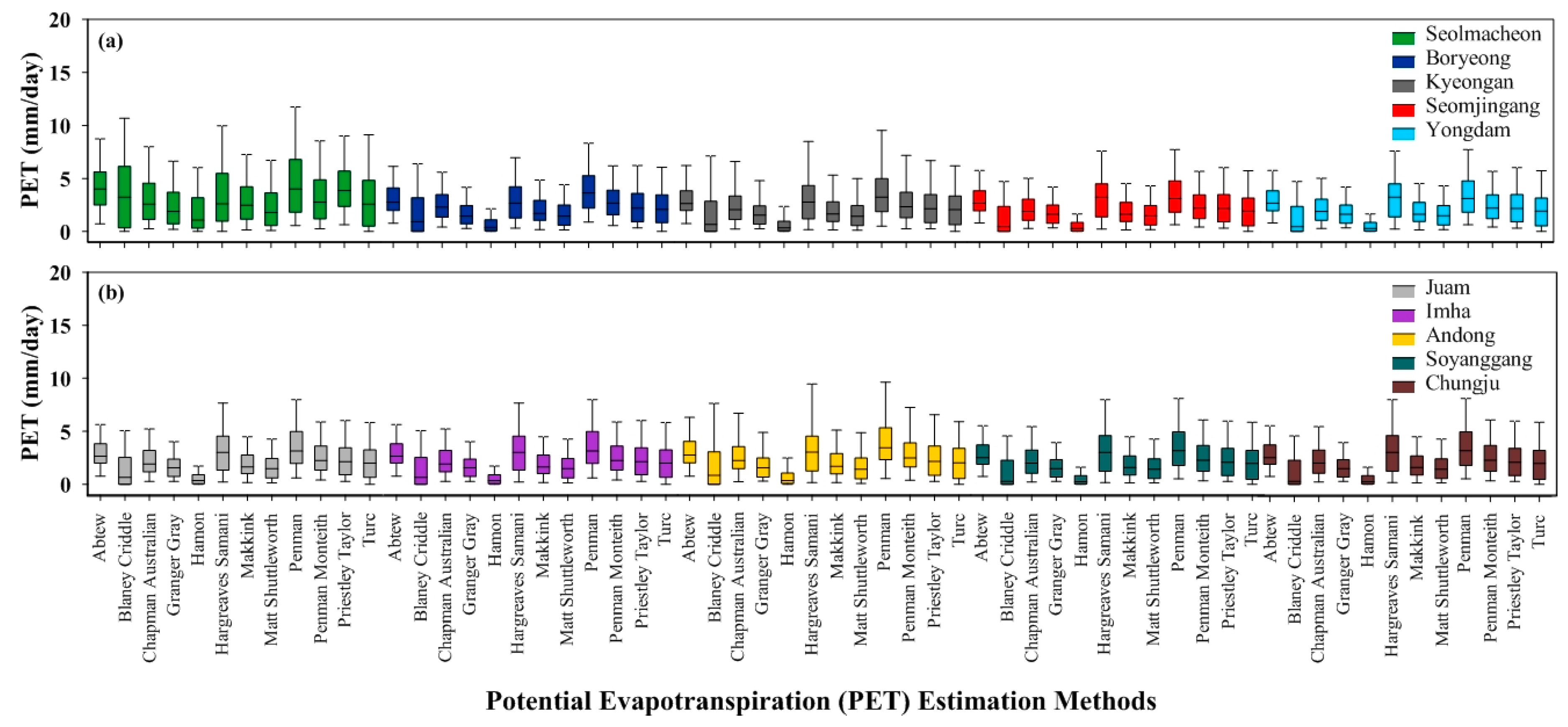
2.3. PET Estimation Methods

Long-term estimation of Actual Evapotranspiration (AET) requires sophisticated techniques or eddy flux instrumentation, which is expensive, and it is more challenging than quantifying the magnitude of PET and other hydro-meteorological parameters [23,53]. Hence, hydrologists interested in applying conceptual rainfall-runoff models often give more emphasis to PET estimation. There are several PET estimation methods with various development philosophies and climate data needs. Xu and Singh [54] grouped the PET estimation methods into five categories: (i) combination, (ii) water budget, (iii) mass-transfer, (iv) radiation, and (v) temperature-based methods. In this study, 12 PET estimation methods with different levels of complexity were applied as inputs to five hydrological models. Guo et al.’s [23] R “evapotranspiration” package was used to estimate the input values of 12 PET over the application periods. The Blaney Criddle, Chapman Australian, Granger Gray, Matt Shuttleworth, Penman, Penman-Monteith, Priestley Taylor, and Turc estimation method are the most complex equation, which requires more data and the Hargreaves Samani method is the only equation that requires temperature data. The remaining three PET estimation methods (Abtew, Hamon, and Makkink) require at least two climate data.

The PET methods selected in this study were only intended to meet the research objectives and the detailed evaporation process, theory, history, and applications of the PET estimation methods have been intensively discussed in several hydrological studies [53,54,55,56]. The PET estimation methods used, including the equation and climate data required, are summarized in

Table A1. List of the 12 PET estimation methods and the required climate data.

PET Estimation Methods	Formula	Required Data	Reference
Abtew	$PET=0.52\frac{R_s}{\lambda }$	T, Rs	[112]
Blaney Criddle	$PET=\left(0.0043R{H}_{min}-\frac{n}{N}-1.41\right)+b_{var }{p}_y\left(0.46T_a+8.13\right)$	T, RH, n	[113]
Chapman Australian	$PET=A_p{E}_{pan}+B_p$	T, RH, Rs	[114]
	$E_{pan}=\frac{\Delta }{\Delta +a_p\gamma }\frac{R_{Npan}}{\lambda }+\frac{a_p\gamma }{\Delta +a_p\gamma }{f}_{pan}\left(u\right)(v_a{}^{*}-v_{a)}$
Granger Gray	$PET=\frac{\Delta G_g}{\Delta G_g+\gamma }\frac{R_n-G}{\lambda }+\frac{\gamma G_g}{\Delta G_g+\gamma }{E}_a$	T, RH, Rs	[115]
Hamon	$PET=0.55{(\frac{n}{12})}^2(\frac{SVD}{100})\left(25.4\right)$	T, n	[116]
Hargreaves Samani	$PET=0.0135C_{HS}\frac{R_a}{\lambda }\left(T_{max}-T_{min}{)}^2(T_a+17.8\right)$	T	[117]
Makkink	$PET=0.61(\frac{\Delta }{\Delta +\gamma }-\frac{R_a}{2.45})-0.12$	T, Rs	[118]
Matt Shuttleworth	$PET=\frac{1}{\lambda }\frac{\Delta R_n+\frac{{\rho }_a{c}_a{u}_2(VP{D}_2)}{r_c{}^{50}}(\frac{VP{D}_{50}}{VP{D}_2})}{\Delta +\gamma (1+\frac{{(r_s)}_c{u}_2}{r_c{}^{50}})}$	T, RH, Rs, u	[119]
Penman	$PET\approx 0.047R_S(T_a+9.5{)}^{0.5}-2.4{(\frac{R_S}{R_a})}^2+0.09(T_a+20)(1-\frac{R{H}_{mean}}{100})$	T, RH, Rs	[120]
Penman-Monteith	$PET=\frac{0.408\Delta \left(R_n-G\right)+\gamma \frac{900}{T_a+273}{u}_{2 }(v_a{}^{*}-v_{a)}}{\Delta +\gamma \left(1+0.34u_{2 }\right)}$	T, RH, Rs, n, u	[121]
Priestley Taylor	$PET=\frac{1.26\Delta R_n}{\lambda \rho \left(\Delta +\gamma \right)}$	T, RH, Rs	[122]
Turc	$PET=0.013\left(23.88R_s+50\right)\left(\frac{T_a}{T_a+15}\right)$, for RH > 50%	T, RH, Rs	[123]
	$PET=0.013\left(23.88R_s+50\right)\left(\frac{T_a}{T_a+15}\right)\left(1+\frac{50-RH}{70}\right)$, for RH < 50%

(Appendix A). The daily PET values of the nine catchments (Seolmacheon, Boryeong, Seomjingang, Yongdam, Juam, Imha, Andong, Soyanggang, and Chungju) were estimated using 12 year climate data (2001–2012) and for the Kyeongan Catchment, 11 year climate data (1998–2008) were used. The Hamon PET estimation method underestimated the daily PET values in all catchments. However, the estimated mean annual PET was identical for the remaining methods. The daily PET values also showed identical patterns and the values were less than 10 mm/day, except for a few outlier values. The estimated daily PET input values for the 10 catchments are presented in Figure 3.

2.4. Overview of Hydrological Model Structure

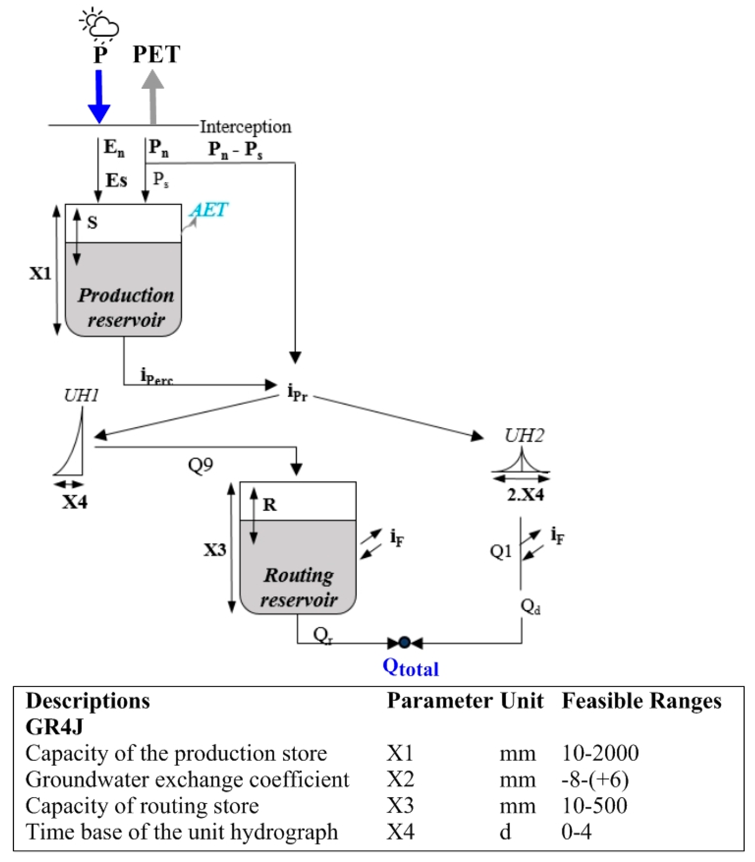
In this study, the GR4J, SIMHYD, CAT, TANK, and SAC-SMA models of increasing complexity with identical input data, including daily precipitation (P) and 12 PET inputs were applied over 10 Korean catchments to assess their effect on model performance, robustness, and optimized parameters. The detailed description of the five hydrological models and the parameters used for calibration are presented in Figure A1, Figure A2, Figure A3, Figure A4 and Figure A5 (Appendix B). The RS MINERVE tool that was developed at the Research Center On Alpine Environment (CREALP) was used to set up the SAC-SMA model; currently, the RS MINERVE platform is providing flood predictions for the Rhone River Basin located in Switzerland [57]. The Catchment Hydrological Cycle Assessment Tool (CAT) Version 3 software, as developed at KICT, was used to set up the GR4J, SIMHYD, CAT, and TANK models [51,52,53].

2.4.1. GR4J

The GR4J model is a conceptual rainfall-runoff model with a parsimonious structure with only four parameters [15]. The rainfall-runoff process starts by separating the rainfall depth and PET to net rainfall or net evapotranspiration capacity depending on the interception storage capacity level. After the separation, the production store capacity, the routing reservoir, lag time, and the groundwater exchange amounts are computed based on the governing equations. Evapotranspiration in the GR4J model occurs only from the production store. The percolated water from the production store is transformed into two unit hydrographs. The routing store uses the input discharge from one of the unit hydrographs, after that, the routing reservoir is emptied by a routing discharge. The groundwater exchange only occurs from the routing reservoir. The model has been tested intensively in several basins and climatic conditions, moreover, there exists several hydrological studies [7,58,59,60,61,62]. The feasible ranges of the four parameters used to calibrate the model for each PET input in the tested catchments were adopted from previous works [15,58,63]. The detailed description of the GR4J model and the parameters that were used for calibration is presented in Figure A1 (Appendix B).

2.4.2. SIMHYD

The SIMHYD model is a daily conceptual rainfall-runoff model adopted from a similar model developed by Porter and McMahon [64]. The SIMHYD model used in this study had seven parameters to simulate the rainfall-runoff response for each PET input [65,66]. The rainfall-runoff conceptualization considers the runoff from impervious areas and infiltration excess modelled as a nonlinear function of soil moisture. The remaining two-process, interflow and base flow from the groundwater store, are modelled when considering linear relationships. In the SIMHYD model, daily evaporation starts from the interception store depending on the availability of water. The model was tested in Australia, the United States, and France for different applications [66,67,68,69,70]. Furthermore, the Australia National Land and Water Resources Audit regularly uses the model to estimate runoff [71]. Chiew et al. [65] provided a detailed technical description of the rainfall-runoff process. The lower and upper limits of all the parameters used to calibrate the model for 12 different PET inputs were selected from previous work [65,67]. The detailed description of the SIMHYD model and the parameters used for calibration is shown in Figure A2 (Appendix B).

2.4.3. CAT

The CAT model is a physically based semi-distributed hydrological model developed to assess the water cycle and the impacts of impervious cover change on storm runoff [72,73,74]. The model is capable of simulating the hydrological components, including AET, soil moisture content, base flow, and runoff from a daily to a sub-daily time step. The main physical parameters that are required for initial simulation are slope, soil types, land use, aquifer, and river information. The conceptualization and development of the basic model were based on the unconfined aquifer and single soil layer assumptions. The model first separates the incoming precipitation that falls on impervious, pervious, and paddy areas. Subsequently, the three areas transform the precipitation to surface flow, infiltration, and evapotranspiration based on the governing equations. The infiltration process can be simulated using Rainfall Excess, Horton, and Green-Ampt models. The groundwater movement computation is based on the Darcy law. Furthermore, the Muskingum, Muskingum-Cunge, and Kinematic wave methods are also included for channel routing. The evapotranspiration in the CAT model depends on the land use and it is composed of plant transpiration as well as evaporation from the surface and soil layer. In this study, the infiltration process is modeled using the Green-Ampt method [75] and lumped hydrological models are considered to represent the rainfall-runoff process. The model has been applied to assess the impacts of urbanization on storm runoff in the north of Swindon town, UK [73]. Recently, Jang et al. [76] applied the CAT model to assess the impact of climate change impact on the hydrological cycle and water management practices while considering A1B and B1 scenarios. The model has also been applied to predict reservoir water levels, to analyze the water cycle, and for flood event simulations [77,78,79]. The main hydrological processes of the CAT model and the parameters that are used for calibration are presented in Figure A3 (Appendix B).

2.4.4. TANK

The TANK model is a conceptual rainfall-runoff model that was originally developed while considering the hydrological conditions of Japan. The TANK model has a series of four tanks arranged in order with 12 parameters [80]. The soil moisture storage tanks transform the catchment rainfall to streamflow by collecting water from each storage tank [81]. The rainfall enters the first tank, which drains free water at two outlets on the side (surface discharge) and the infiltrated water from soil moisture drains downward to the bottom outlet. The infiltrated water from the first tank enters the second tank; the second tank drains the free water to the side outlet (intermediate discharge) and the percolated water drains downward to the bottom outlet to enter the third tank. Similarly, the third tank drains the sub-base discharge to the side outlet and the deep percolated water drains the remaining water to the fourth tank. The lowermost tank drains the water at one side of the tank outlet (base discharge) and it often contributes a small portion of the total outflow. However, the water that drains from the three side tanks contributes a considerable amount of total outflow. Evapotranspiration is able to occur from the four tanks. Sugawara [82] discussed the rainfall-runoff and calibration process in detail. The model has been widely applied in many Asian countries and other basins for various applications [83,84,85,86]. The twelve feasible parameter ranges used to calibrate the TANK model were adopted from earlier works [82,87]. The TANK model description and the parameters that were used for calibration are presented in Figure A4 (Appendix B).

2.4.5. SAC-SMA

The SAC-SMA model is a soil moisture accounting model with 16 parameters [88] and the most complex model when compared to the other four models that are applied in this study. The SAC-SMA model was originally developed at the California-Nevada River Forecast Center and the U.S. National Weather Service River Forecast System uses it as the main model for forecasting flood events [89]. The model transforms the precipitation that falls on impervious and pervious areas to direct runoff. The remaining water infiltrated from the previous areas to the first soil layer will be changed to tension and free water. The free water drains water to the river through surface runoff or interflow and the remaining water will percolate to the second soil layer. The second soil layer contains three zones to store water: tension water, primary, and supplementary free water. The primary as well as supplementary free water transforms the percolated water to the total river flow via the base flow and subsurface discharge. The surface water and first and second zone tension water stores are able to contribute to total evapotranspiration. Burnash [88] presented a more detailed description of the SAC-SMA model. The SAC-SMA model has also been tested in a wide range of basins and climatic conditions [14,90,91,92,93]. In this study, 13 SAC-SMA model parameters were selected for calibration [89,94,95] and the default values were used for the remaining three parameters across all of the catchments. The feasible parameter ranges for calibration were adopted from a previous study [96]. The detailed description of the SAC-SMA model and the feasible parameters ranges used for calibration are presented in Figure A5 (Appendix B).

2.5. Model Calibration and Validation

Hydrological model calibration can be done manually or automatically while using an optimization algorithm to enhance streamflow simulation and model robustness. There exist different kinds of global optimization algorithms, including the Monte Carlo, Genetic Algorithm, Generalized Likelihood Uncertainty Estimation, Artificial Neural Network, and SCE-UA, which have been used to calibrate hydrological models [97,98]. Similarly, the Latin Hypercube and Rosenbrock algorithms have also been used to calibrate hydrological models [99,100]. Each optimization algorithm has their own benefits and limitations. The SCE-UA global optimization algorithm considers the deterministic and probabilistic approaches. Moreover, the complex shuffling, the systematic evolution of complex points, and competitive evolution makes the algorithm efficient, effective, and robust [49].

In this study, the SCE-UA optimization algorithm of Duan et al. [49] was applied while considering its broad applications, flexibility, robustness, and efficiency [50,51,52,101]. The SCE-UA algorithm was applied to calibrate five hydrological models for 12 different PET inputs when considering four objective functions: NSE, LogNSE, KGE, and RSR. The NSE, LogNSE, KGE, and RSR objective functions have been recommended for evaluating hydrological model performance for streamflow simulation in recent studies [40,41]. The five hydrological models were calibrated while using seven years of observed streamflow data (2002–2008) for nine catchments and the remaining four year data were used for validation (2009–2012). However, the Kyeongan catchment calibration was carried out using the available observed streamflow data (2000–2005) and the remaining data (2006–2008) were used for validation. A one-year warm-up period was considered in all of the tested catchments to minimize the errors at the beginning of the calibration period for all models and their corresponding PET input values. In addition, the five hydrological model performance percentage variations were compared with other PET inputs considering the Penman-Monteith PET input NSE index values as a benchmark. The four objective functions, NSE, LogNSE, KGE, and RSR, were calculated, as follows:

$$\mathrm{NSE}=1-\frac{\sum {({\mathrm{Q}}_{\mathrm{obs}}-{\mathrm{Q}}_{\mathrm{sim}})}^2}{\sum {({\mathrm{Q}}_{\mathrm{obs}}-{\mathrm{Q}}_{\mathrm{mean}})}^2}$$

(1)

$$\mathrm{LogNSE}=1-\frac{\sum {({\mathrm{logQ}}_{\mathrm{obs}}-{\mathrm{logQ}}_{\mathrm{sim}})}^2}{\sum {({\mathrm{logQ}}_{\mathrm{obs}}-{\mathrm{logQ}}_{\mathrm{mean}})}^2}$$

(2)

$$\mathrm{KGE}=1-\sqrt{{(R^2\left[{\mathrm{Q}}_{\mathrm{obs}},{\mathrm{Q}}_{\mathrm{sim}}\right]-1)}^2+(\frac{\mathrm{SD}[{\mathrm{Q}}_{\mathrm{sim}}]}{\mathrm{SD}[{\mathrm{Q}}_{\mathrm{obs}}]}-1){}^2+(\frac{\mathrm{M}[{\mathrm{Q}}_{\mathrm{sim}}]}{\mathrm{M}\left[{\mathrm{Q}}_{\mathrm{obs}}\right]}-1){}^2}$$

(3)

$$\mathrm{RSR}=\frac{\mathrm{RMSE}}{\mathrm{SD}[{\mathrm{Q}}_{\mathrm{obs}}]}=\frac{\sqrt{\sum {({\mathrm{Q}}_{\mathrm{obs}}-{\mathrm{Q}}_{\mathrm{sim}})}^2}}{\sqrt{\sum {({\mathrm{Q}}_{\mathrm{obs}}-{\mathrm{Q}}_{\mathrm{mean}})}^2}}$$

(4)

where Q_obs, Q_sim, and Q_mean are the observed, simulated, and mean observed streamflow, respectively. R², SD, and M are the Pearson Correlation Coefficient, standard deviation, and mean, respectively.

2.6. Model Complexity Comparison Criteria and Robustness

2.6.1. Model Complexity Comparison Criteria

The five hydrological models were further evaluated by comparing three statistical indicators: AIC, BIC, and Ra² for each PET input. The AIC, BIC, and Ra² are the statistical indicators commonly used to compare a model structure of different complexity in various subject areas. The three statistical indicators’ model comparison criteria are able to penalize the number of estimated parameters depending on the model complexity. The model comparison criteria have been applied for frequency analysis of hydrological extremes [46,102] and for predictions of groundwater models [103]. Other studies have also applied the criteria to compare conceptual rainfall-runoff models with artificial neural network models [45,104,105]. Akaike [43] proposed the AIC for the first time based on Kullback-Leibler’s information as the discrepancies between the observed and simulated models. Similarly, Schwarz [44] proposed a more parsimonious method, called the BIC, which considers the Bayesian approaches. The Adjusted R-square Ra² has also been used as an alternative method to compare model structures of different complexity [45]. The AIC, BIC, and Ra² statistical indicators were calculated for the five hydrological models of increasing complexity for each PET input. The model with a minimum AIC, BIC, and maximum Ra² was considered to be the better performing and with greater parsimony. In this study, similar model comparison criteria were adopted to evaluate the five hydrological models for each PET input. The three statistical indicators, AIC, BIC, and Ra² were calculated, as follows:

$$\mathrm{AIC}=\mathrm{nln}\left(\mathrm{RMSE}\right)+2\mathrm{p}$$

(5)

$$\mathrm{BIC}=\mathrm{nln}\left(\mathrm{RMSE}\right)+\mathrm{pln}\left(\mathrm{n}\right)$$

(6)

$${\mathrm{R}}_{\mathrm{a}}{}^2=R^2-\left(\frac{\mathrm{p}-1}{\mathrm{n}-\mathrm{p}}\right)(1-R^2)$$

(7)

where n, RMSE, p, and R² are the number of data points, root mean squared error of the model output, the number of model parameters, and Pearson Correlation Coefficient, respectively.

2.6.2. Model Robustness

Model robustness plays an important role in practical applications to provide reliable results. [106]. Although robustness is an essential quality of any model, hydrological models often tend to perform differently between the calibration and validation periods [7]. Moreover, the parameters of the conceptual rainfall-runoff model often face difficulties in appropriately reproducing the water balances [48]. The importance of minimizing the water balance errors in the model calibration process to enhance hydrological model robustness has been discussed in recent studies [47,48]. The KGE model evaluation criteria consider the various aspects of model behavior, including the water balance error, accuracy, and robustness. Furthermore, Coron et al. [48] investigated the robustness of three rainfall-runoff models regarding water balance simulation and suggested comparing the Dimensionless Bias (the ratio of 10 year mean simulated and observed flows) to evaluate the robustness of three hydrological models of increasing complexity over 20 French catchments. In this study, a similar approach that was suggested by Coron et al. [48] was adopted to evaluate the five hydrological models’ robustness and behavioral similarities for each PET input. The Dimensionless Bias for a robust model is expected to be one. The Dimensionless Bias is calculated, as follows:

$$Dimensionless Bias =\frac{\underset{{\mathrm{Q}}_{\mathrm{sim}}}{\to }}{\underset{{\mathrm{Q}}_{\mathrm{obs}}}{\to }}$$

(8)

where $\underset{{\mathrm{Q}}_{\mathrm{sim}}}{\to }$ and $\underset{{\mathrm{Q}}_{\mathrm{obs}}}{\to }$ are the 10 year mean simulated and observed flows, respectively.

3. Results

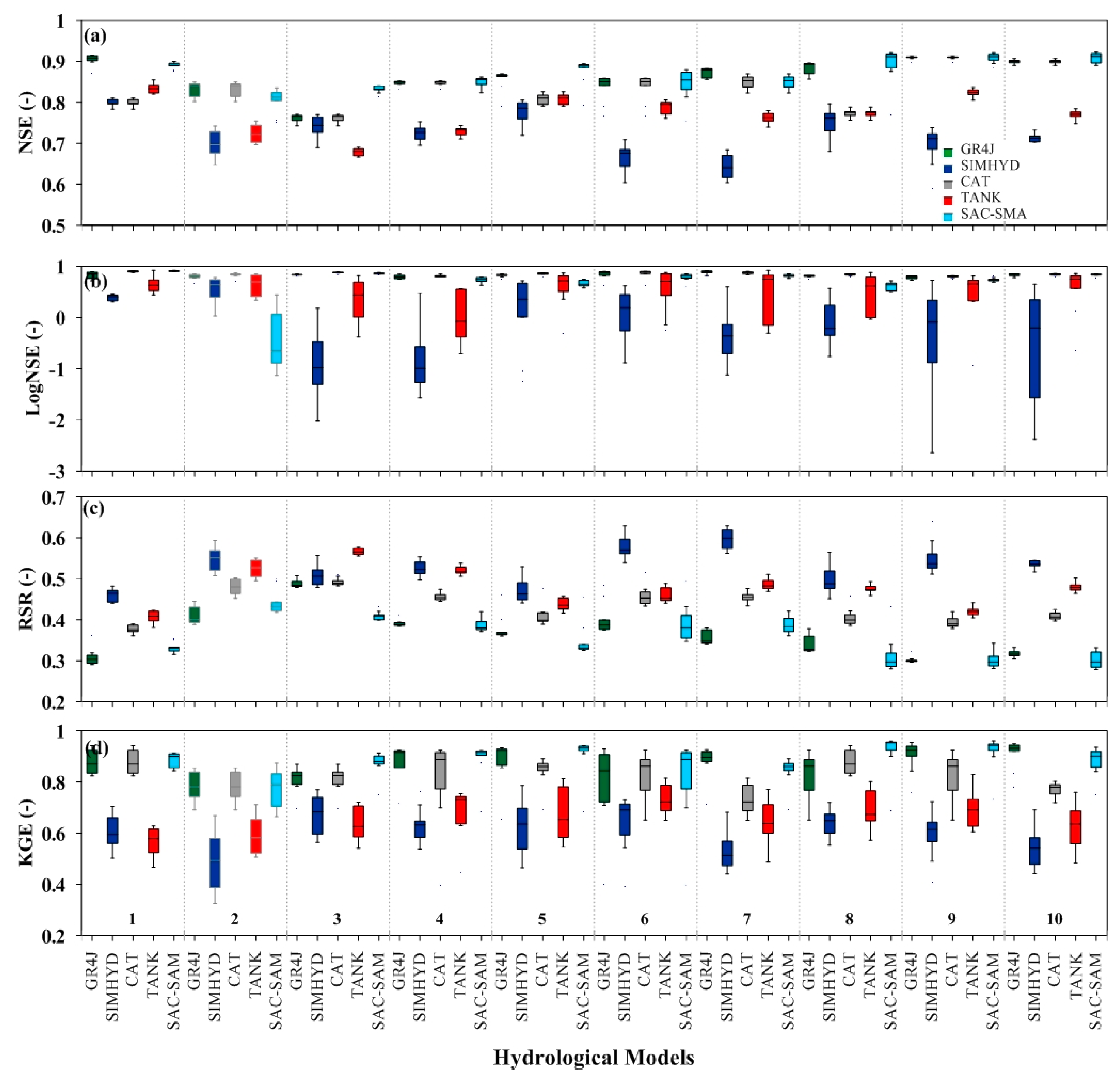
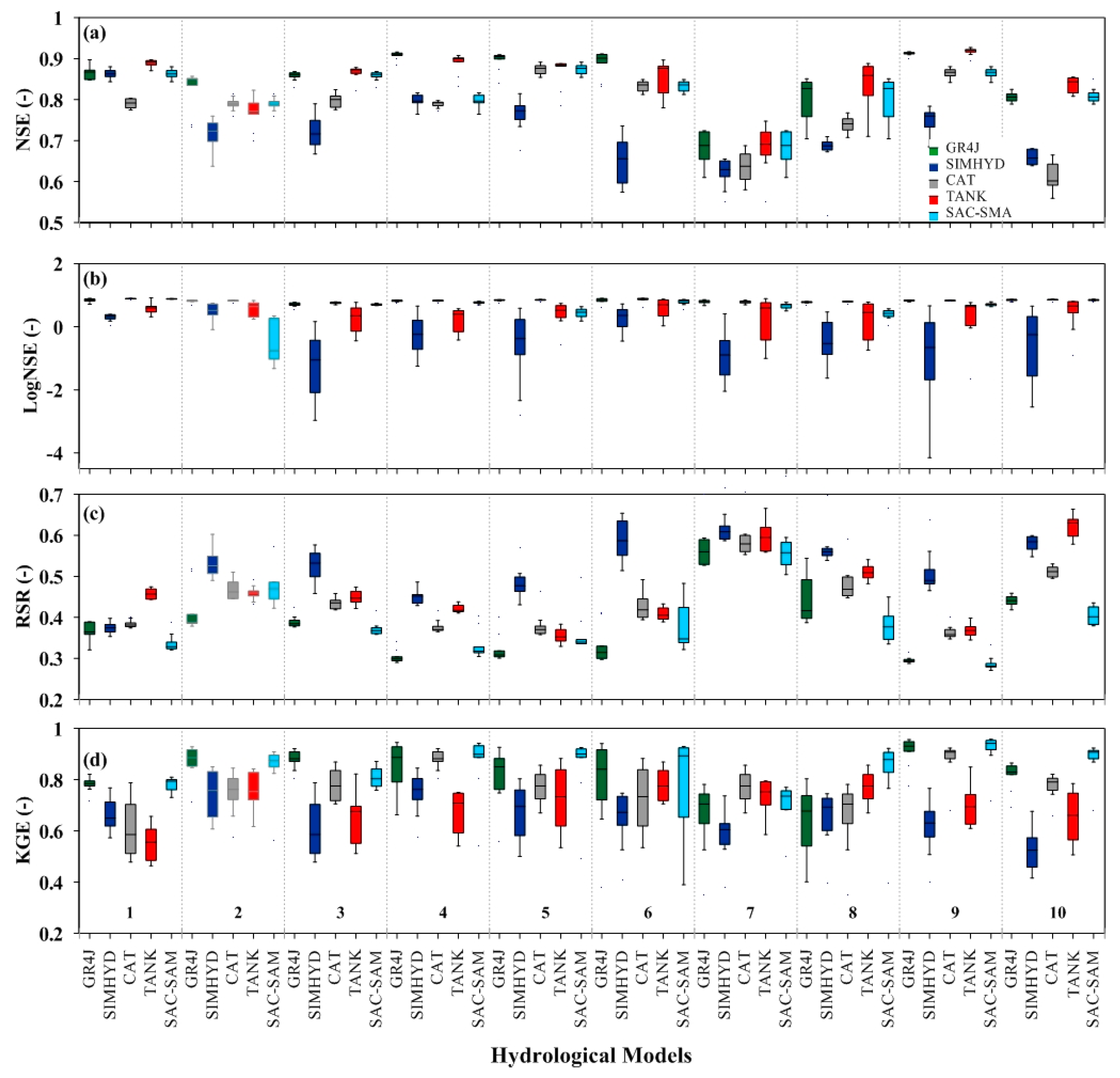
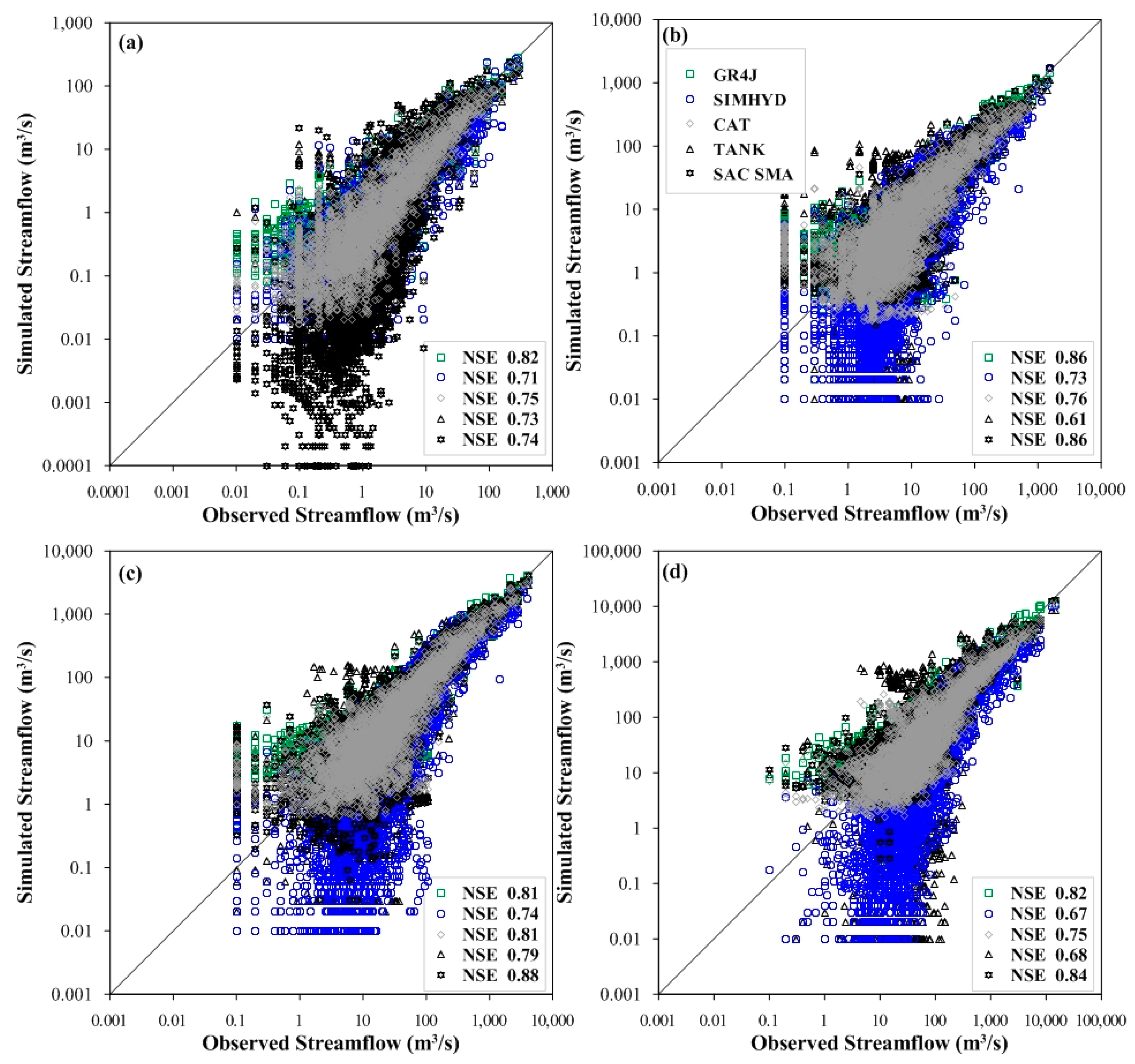
3.1. Calibration and Validation

The model evaluation guidelines of Moriasi et al. [40] recommended a NSE > 0.50 and RSR < 0.70 as satisfactory performance for streamflow simulation. The performance of the GR4J, SIMHYD, CAT, TANK, and SAC-SMA models for the 12 PET inputs were found to be satisfactory for all of the tested catchments in the calibration periods, as shown in Figure 4. Similarly, the performances of the five hydrological models for each PET input fell within satisfactory criteria for all the tested catchments in the validation periods (

Table A2. The performances of the five hydrological models in the validation periods.

Seolmacheon	NSE					LogNSE
PET Methods	GR4J	SIMHYD	CAT	TANK	SAC-SAM	GR4J	SIMHYD	CAT	TANK	SAC-SAM
Abtew	0.85	0.87	0.80	0.89	0.87	0.71	0.18	0.85	0.91	0.87
Blaney Criddle	0.87	0.87	0.79	0.89	0.87	0.87	0.29	0.88	0.62	0.87
Chapman Australian	0.86	0.87	0.78	0.90	0.87	0.83	0.38	0.89	0.57	0.89
Granger Gray	0.90	0.84	0.80	0.89	0.84	0.87	0.31	0.88	0.47	0.89
Hamon	0.87	0.86	0.80	0.89	0.86	0.88	0.37	0.89	0.62	0.89
Hargreaves Samani	0.87	0.86	0.77	0.88	0.86	0.88	0.03	0.90	0.49	0.89
Makkink	0.85	0.85	0.80	0.90	0.85	0.81	0.34	0.88	0.32	0.88
Matt Shuttleworth	0.87	0.86	0.78	0.90	0.86	0.89	0.39	0.90	0.63	0.89
Penman	0.87	0.88	0.79	0.88	0.88	0.83	0.35	0.88	0.55	0.88
Penman-Monteith	0.86	0.87	0.79	0.89	0.87	0.84	0.38	0.89	0.45	0.88
Priestley Taylor	0.85	0.86	0.78	0.87	0.86	0.73	0.25	0.85	0.76	0.87
Turc	0.88	0.86	0.80	0.89	0.86	0.90	0.39	0.90	0.65	0.88
Boryeong
Abtew	0.85	0.66	0.79	0.77	0.79	0.82	0.46	0.81	0.24	0.15
Blaney Criddle	0.85	0.72	0.79	0.77	0.79	0.80	0.75	0.83	0.72	−1.33
Chapman Australian	0.86	0.76	0.76	0.82	0.76	0.84	0.46	0.84	0.25	−0.71
Granger Gray	0.85	0.74	0.79	0.77	0.79	0.81	0.72	0.83	0.62	−1.00
Hamon	0.83	0.64	0.79	0.70	0.79	0.68	0.65	0.73	0.42	0.29
Hargreaves Samani	0.74	0.74	0.79	0.79	0.79	0.82	0.23	0.84	0.31	0.34
Makkink	0.85	0.72	0.81	0.76	0.81	0.84	0.63	0.85	0.66	−0.82
Matt Shuttleworth	0.85	0.70	0.81	0.79	0.81	0.80	0.74	0.82	0.83	−1.03
Penman	0.85	0.75	0.78	0.72	0.78	0.83	−0.09	0.82	0.59	0.27
Penman-Monteith	0.86	0.74	0.80	0.80	0.80	0.84	0.40	0.82	0.74	−0.40
Priestley Taylor	0.85	0.73	0.79	0.79	0.79	0.83	0.38	0.84	0.77	−1.07
Turc	0.73	0.71	0.77	0.77	0.77	0.80	0.57	0.85	0.75	−0.87
Kyeongan
Abtew	0.85	0.79	0.78	0.87	0.85	0.65	−2.15	0.73	0.77	0.70
Blaney Criddle	0.86	0.75	0.82	0.87	0.86	0.76	0.16	0.77	0.49	0.70
Chapman Australian	0.86	0.72	0.80	0.87	0.86	0.70	−2.09	0.74	0.66	0.68
Granger Gray	0.87	0.72	0.80	0.88	0.87	0.75	−0.43	0.75	0.55	0.68
Hamon	0.86	0.70	0.82	0.82	0.86	0.77	0.15	0.79	0.60	0.75
Hargreaves Samani	0.86	0.72	0.78	0.86	0.86	0.68	−1.54	0.74	−0.45	0.71
Makkink	0.86	0.71	0.80	0.87	0.86	0.72	−1.00	0.74	−0.03	0.67
Matt Shuttleworth	0.87	0.76	0.80	0.88	0.87	0.76	−0.52	0.78	0.42	0.72
Penman	0.83	0.69	0.78	0.86	0.83	0.53	−1.64	0.69	−0.14	0.72
Penman-Monteith	0.86	0.71	0.79	0.87	0.86	0.68	−2.97	0.75	0.05	0.72
Priestley Taylor	0.86	0.67	0.81	0.87	0.86	0.72	−1.11	0.76	0.27	0.72
Turc	0.87	0.68	0.81	0.87	0.87	0.76	−0.50	0.79	−0.18	0.73
Seomjingang
Abtew	0.91	0.81	0.80	0.90	0.81	0.83	−0.72	0.83	−0.32	0.79
Blaney Criddle	0.90	0.79	0.79	0.86	0.79	0.79	0.66	0.80	0.57	0.68
Chapman Australian	0.91	0.79	0.79	0.90	0.79	0.84	−0.02	0.84	0.37	0.78
Granger Gray	0.91	0.80	0.79	0.90	0.80	0.83	0.05	0.83	0.51	0.76
Hamon	0.88	0.76	0.77	0.83	0.76	0.73	0.64	0.73	0.42	0.70
Hargreaves Samani	0.92	0.79	0.78	0.89	0.79	0.84	−0.50	0.83	−0.16	0.76
Makkink	0.91	0.81	0.79	0.90	0.81	0.84	0.20	0.84	0.44	0.79
Matt Shuttleworth	0.91	0.80	0.79	0.91	0.80	0.80	−0.13	0.83	0.57	0.80
Penman	0.92	0.82	0.79	0.90	0.82	0.84	−1.25	0.84	−0.42	0.78
Penman-Monteith	0.91	0.79	0.79	0.90	0.79	0.84	−0.93	0.84	0.10	0.77
Priestley Taylor	0.91	0.79	0.79	0.89	0.79	0.84	−0.55	0.83	0.29	0.75
Turc	0.91	0.80	0.79	0.90	0.80	0.82	−0.36	0.82	0.47	0.76
Yongdam
Abtew	0.91	0.79	0.89	0.89	0.89	0.85	−2.80	0.86	0.49	0.46
Blaney Criddle	0.90	0.73	0.87	0.82	0.87	0.81	0.47	0.86	0.55	0.32
Chapman Australian	0.91	0.78	0.89	0.89	0.89	0.85	−0.87	0.86	0.19	0.18
Granger Gray	0.90	0.78	0.88	0.89	0.88	0.84	−0.09	0.84	0.64	0.46
Hamon	0.84	0.68	0.85	0.78	0.85	0.75	0.59	0.77	0.29	0.33
Hargreaves Samani	0.91	0.75	0.86	0.88	0.86	0.86	−0.76	0.86	−0.57	0.55
Makkink	0.90	0.77	0.88	0.89	0.88	0.85	0.23	0.86	0.63	0.33
Matt Shuttleworth	0.90	0.76	0.88	0.88	0.88	0.84	0.17	0.85	0.67	0.33
Penman	0.91	0.78	0.86	0.88	0.86	0.86	−2.34	0.85	0.73	0.64
Penman-Monteith	0.91	0.77	0.88	0.88	0.88	0.86	−0.67	0.86	0.46	0.56
Priestley Taylor	0.91	0.81	0.87	0.88	0.87	0.85	−0.88	0.85	0.68	0.52
Turc	0.87	0.79	0.87	0.89	0.87	0.83	0.10	0.84	0.34	0.46
Juam
Abtew	0.90	0.66	0.84	0.88	0.84	0.88	−0.46	0.90	0.85	0.86
Blaney Criddle	0.90	0.57	0.83	0.81	0.83	0.82	0.72	0.87	0.67	0.70
Chapman Australian	0.91	0.67	0.81	0.88	0.81	0.89	0.37	0.90	0.79	0.80
Granger Gray	0.90	0.70	0.81	0.84	0.81	0.81	0.41	0.86	0.56	0.84
Hamon	0.84	0.57	0.82	0.78	0.82	0.61	0.20	0.60	0.73	0.52
Hargreaves Samani	0.89	0.74	0.83	0.90	0.83	0.89	−0.07	0.90	0.03	0.75
Makkink	0.91	0.60	0.85	0.84	0.85	0.86	0.54	0.90	0.87	0.85
Matt Shuttleworth	0.90	0.60	0.85	0.82	0.85	0.80	0.56	0.86	0.85	0.77
Penman	0.90	0.72	0.84	0.89	0.84	0.86	0.00	0.87	0.67	0.80
Penman-Monteith	0.91	0.69	0.84	0.88	0.84	0.90	0.15	0.89	0.08	0.85
Priestley Taylor	0.91	0.63	0.84	0.88	0.84	0.88	0.40	0.89	0.34	0.82
Turc	0.83	0.66	0.83	0.88	0.83	0.85	0.35	0.87	0.81	0.81
Imha
Abtew	0.69	0.61	0.64	0.67	0.69	0.70	−1.53	0.73	0.89	0.70
Blaney Criddle	0.65	0.58	0.67	0.71	0.65	0.83	0.41	0.83	0.74	0.70
Chapman Australian	0.72	0.65	0.65	0.71	0.72	0.78	−1.35	0.80	−1.00	0.78
Granger Gray	0.67	0.62	0.60	0.66	0.67	0.82	−0.44	0.80	−0.03	0.71
Hamon	0.61	0.55	0.58	0.55	0.61	0.67	0.37	0.70	0.61	0.67
Hargreaves Samani	0.65	0.63	0.62	0.67	0.65	0.80	−1.11	0.79	0.76	0.71
Makkink	0.70	0.62	0.64	0.72	0.70	0.80	−0.63	0.78	−0.61	0.65
Matt Shuttleworth	0.69	0.65	0.69	0.75	0.69	0.84	−1.76	0.81	0.59	0.50
Penman	0.65	0.65	0.61	0.65	0.65	0.79	−0.77	0.78	0.59	0.71
Penman-Monteith	0.72	0.65	0.68	0.67	0.72	0.76	−2.05	0.75	0.86	0.60
Priestley Taylor	0.70	0.63	0.62	0.72	0.70	0.82	−1.03	0.80	−0.42	0.56
Turc	0.72	0.63	0.67	0.72	0.72	0.86	−0.76	0.84	−0.30	0.71
Andong
Abtew	0.83	0.69	0.74	0.84	0.83	0.79	−1.63	0.80	0.78	0.51
Blaney Criddle	0.70	0.68	0.73	0.86	0.70	0.76	0.46	0.80	0.61	0.57
Chapman Australian	0.84	0.69	0.75	0.88	0.84	0.80	−0.88	0.81	−0.38	0.35
Granger Gray	0.82	0.69	0.73	0.86	0.82	0.76	−0.18	0.79	0.30	0.29
Hamon	0.75	0.52	0.75	0.71	0.75	0.67	0.43	0.71	0.72	0.39
Hargreaves Samani	0.85	0.69	0.71	0.81	0.85	0.80	−0.88	0.79	−0.74	0.40
Makkink	0.83	0.71	0.73	0.89	0.83	0.78	−0.45	0.81	−0.42	0.33
Matt Shuttleworth	0.83	0.70	0.77	0.89	0.83	0.76	0.14	0.79	0.68	0.03
Penman	0.84	0.67	0.75	0.84	0.84	0.80	−0.93	0.80	0.11	0.51
Penman-Monteith	0.84	0.69	0.74	0.88	0.84	0.80	−0.81	0.81	−0.57	0.48
Priestley Taylor	0.83	0.70	0.74	0.86	0.83	0.78	−0.61	0.80	0.73	0.52
Turc	0.76	0.68	0.76	0.80	0.76	0.76	−0.08	0.79	0.66	0.45
Soyanggang
Abtew	0.91	0.77	0.86	0.92	0.86	0.84	−1.47	0.82	−1.66	0.71
Blaney Criddle	0.91	0.75	0.88	0.92	0.88	0.80	0.55	0.84	0.69	0.79
Chapman Australian	0.91	0.76	0.87	0.93	0.87	0.84	−0.52	0.84	0.66	0.73
Granger Gray	0.91	0.76	0.86	0.92	0.86	0.83	−0.15	0.83	0.65	0.63
Hamon	0.90	0.77	0.88	0.90	0.88	0.79	0.66	0.80	0.77	0.72
Hargreaves Samani	0.91	0.75	0.84	0.92	0.84	0.84	−1.68	0.83	0.03	0.66
Makkink	0.91	0.73	0.86	0.92	0.86	0.84	−1.78	0.84	0.68	0.71
Matt Shuttleworth	0.91	0.69	0.86	0.92	0.86	0.83	−0.80	0.83	0.68	0.67
Penman	0.92	0.62	0.87	0.91	0.87	0.84	−4.15	0.82	−0.04	0.71
Penman-Monteith	0.91	0.76	0.87	0.92	0.87	0.84	−1.06	0.83	0.46	0.71
Priestley Taylor	0.91	0.78	0.87	0.92	0.87	0.83	−0.45	0.82	0.62	0.68
Turc	0.92	0.78	0.87	0.92	0.87	0.82	0.13	0.82	0.47	0.73
Chungju
Abtew	0.79	0.66	0.60	0.84	0.79	0.86	−1.67	0.86	0.80	0.83
Blaney Criddle	0.82	0.64	0.65	0.85	0.82	0.79	0.65	0.85	0.73	0.86
Chapman Australian	0.80	0.65	0.59	0.86	0.80	0.86	−0.87	0.87	−0.09	0.86
Granger Gray	0.81	0.66	0.66	0.85	0.85	0.85	0.33	0.86	0.44	0.86
Hamon	0.80	0.68	0.62	0.81	0.80	0.77	0.65	0.78	0.80	0.78
Hargreaves Samani	0.80	0.68	0.56	0.82	0.80	0.86	−1.56	0.86	0.70	0.85
Makkink	0.81	0.66	0.59	0.85	0.81	0.86	−0.23	0.87	0.68	0.87
Matt Shuttleworth	0.81	0.68	0.64	0.85	0.81	0.84	0.32	0.86	0.58	0.86
Penman	0.79	0.64	0.61	0.84	0.79	0.86	−2.55	0.86	0.79	0.85
Penman-Monteith	0.80	0.64	0.62	0.82	0.80	0.86	−1.09	0.86	−0.92	0.84
Priestley Taylor	0.81	0.64	0.58	0.81	0.81	0.85	−0.28	0.86	0.64	0.82
Turc	0.83	0.68	0.60	0.85	0.83	0.83	0.14	0.85	0.51	0.86

in Appendix A), as shown in Figure 5 and Figure A6 (Appendix B). The Hamon PET estimation method relatively underestimated the daily PET values in all catchments (Figure 3), and the response of the five hydrological models also clearly showed the minimum performance, except for the Seolmacheon catchment. Figure 4 shows the model performances (NSE, LogNSE, RSR, and KGE) in the calibration periods for the 12 PET input values.

The comparison of Figure 4 and Figure 5 clearly shows the existence of minor model performance variation between the calibration and validation periods. The variation depends on the hydrological model structures, PET inputs, hydrological characteristics, and climatic conditions of the 10 tested catchments. In the case of NSE and RSR, for example, the variation ranged from 0.1 to 0.2. However, in the case of KGE, the variation ranged from 0.1 to 0.35 in the calibration as well as validation periods. The variation of the NSE, LogNSE, RSR, and KGE index values indicates the existence of model stability or the robustness difference in the calibration and validation periods (Figure 4 and Figure 5). The GR4J, SIMHYD, CAT, TANK, and SAC-SMA hydrological model performances for the 12 PET inputs for the 10 tested catchments are shown in Figure 4 and Figure 5. Figure 4 shows the model performances (NSE, LogNSE, RSR, and KGE) in the validation periods for the 12 PET input values.

The five hydrological model performance percentage variations, calculated while considering the Penman-Monteith PET input NSE index values as benchmark, showed a maximum drop of 17% in the Soyanggang catchment when the SIMHYD model was applied using the Penman PET input. However, a maximum rise of 11% was observed in the Boryang catchment when the SAC-SMA model was applied using the Makkink PET input in the calibration period (Figure A6 in Appendix B). Similarly, the five hydrological model performance percentage variations computed when considering identical assumption showed a maximum drop of 19% in the Soyanggang catchment when the SIMHYD model was applied while using the Penman PET input and a maximum rise of 6.5% was observed in the Chungju catchment when the SAC-SMA model was applied using the Granger Gray PET input in the validation period, as shown in Figure 6. The five hydrological model performance percentage variations calculated when considering the Penman-Monteith PET input NSE index values as a benchmark for four selected catchments in the validation period are presented in Figure 6.

The GR4J, CAT, and SAC-SMA hydrological models’ NSE, RSR, KGE, and R² assessment criterion showed relatively higher values when compared to the SIMHYD and TANK models in most of the tested catchments in the calibration as well as the validation periods. However, it would be naive to identify one best hydrological model because of the minor differences in the index values (NSE < 0.2, RSR < 0.15, KGE < 0.2, and R² < 0.15) in most of the tested catchments, except for the Imha and Andong catchments. The five hydrological models’ performance was observed to be higher and more insensitive for the Seolmacheon experimental catchment for the 12 PET inputs in the calibration and validation periods (Figure 4 and Figure 5). The scatterplot of the five hydrological models’ performance simulated over the application period (2002–2012) for four selected catchments when considering the Penman-Monteith PET input also showed a small variation (R² < 0.15), as presented in Figure 7.

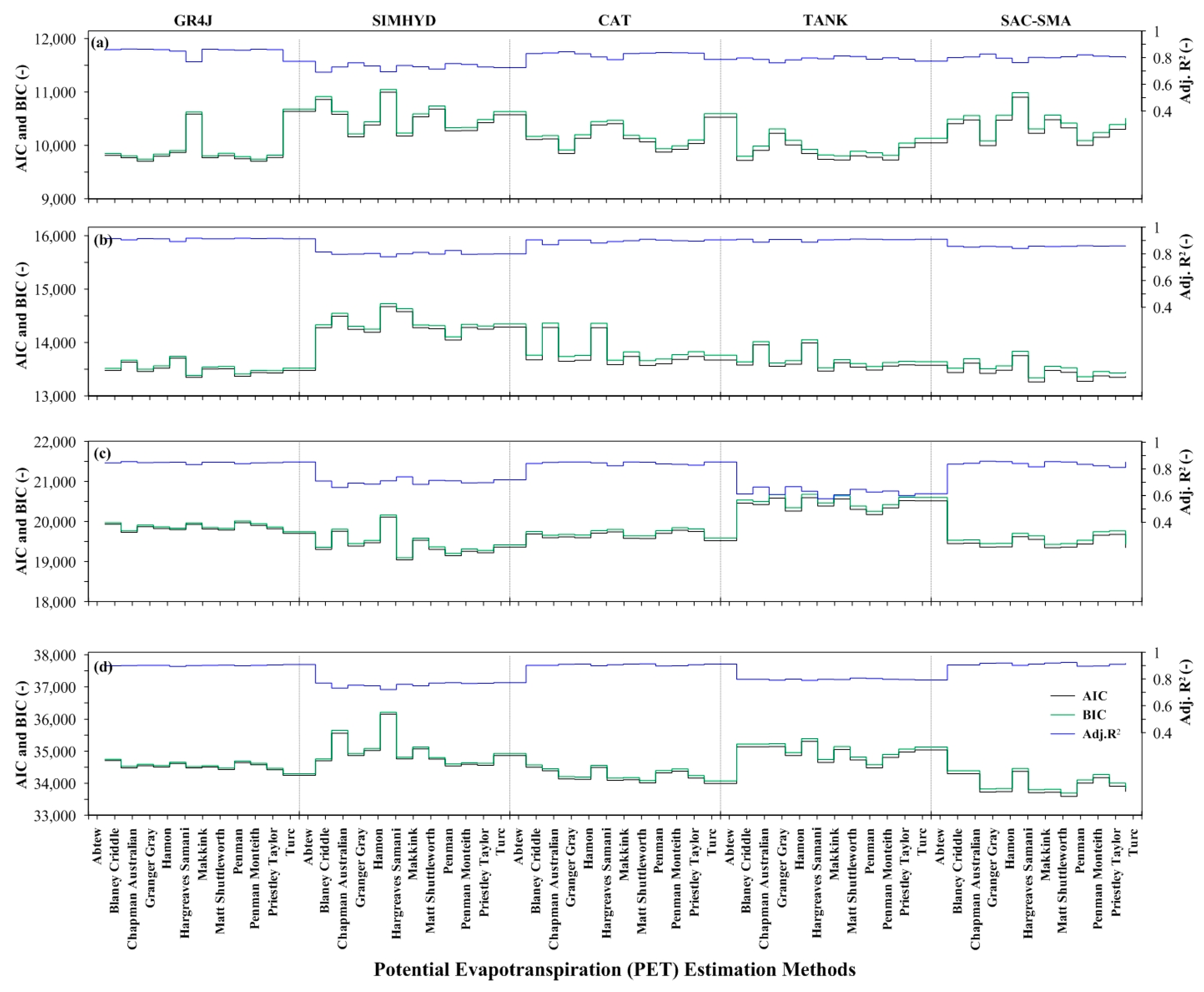
3.2. Effect of Model Structure Complexity on Model Performance

The GR4J, CAT, and SAC-SMA models showed a consistent and better model performance in all of the tested catchments both in the calibration and validation periods. The GR4J, CAT, and SAC-SMA models’ performance response to the 12 PET inputs showed a similar pattern and magnitude of NSE, LogNSE, RSR, and KGE, as shown in Figure 4 and Figure 5. The SIMHYD model performed less when compared to the GR4J, CAT, TANK, and SAC-SMA models in most of the tested catchments. However, for the SIMHYD model, consistent and comparable performances were observed for the Kyeongan, Seomjingang, and Andong catchments in the calibration periods. Similar responses were also observed for the Seolmacheon, Seomjingang, and Chungju catchments in the validation periods. The TANK model performed relatively better than the SIMHYD model, except for the Kyeongan, Seomjingang, and Andong catchments in the calibration periods, and the Seolmacheon, Seomjingang, and Chungju catchments in the validation periods. The GR4J, SIMHYD, CAT, TANK, and SAC-SMA models responses to 12 different PET inputs showed a minor difference (NSE < 0.2) in terms of the NSE index value in all of the tested catchments. Although the SIMHYD model response to 12 PET inputs showed a minor difference (NSE < 0.2), unstable patterns of NSE were observed, except in the Seolmacheon experimental catchment. The five hydrological models’ performance for four selected catchments simulated over the application periods (2002–2012) for the 12 PET inputs are shown in Figure 8.

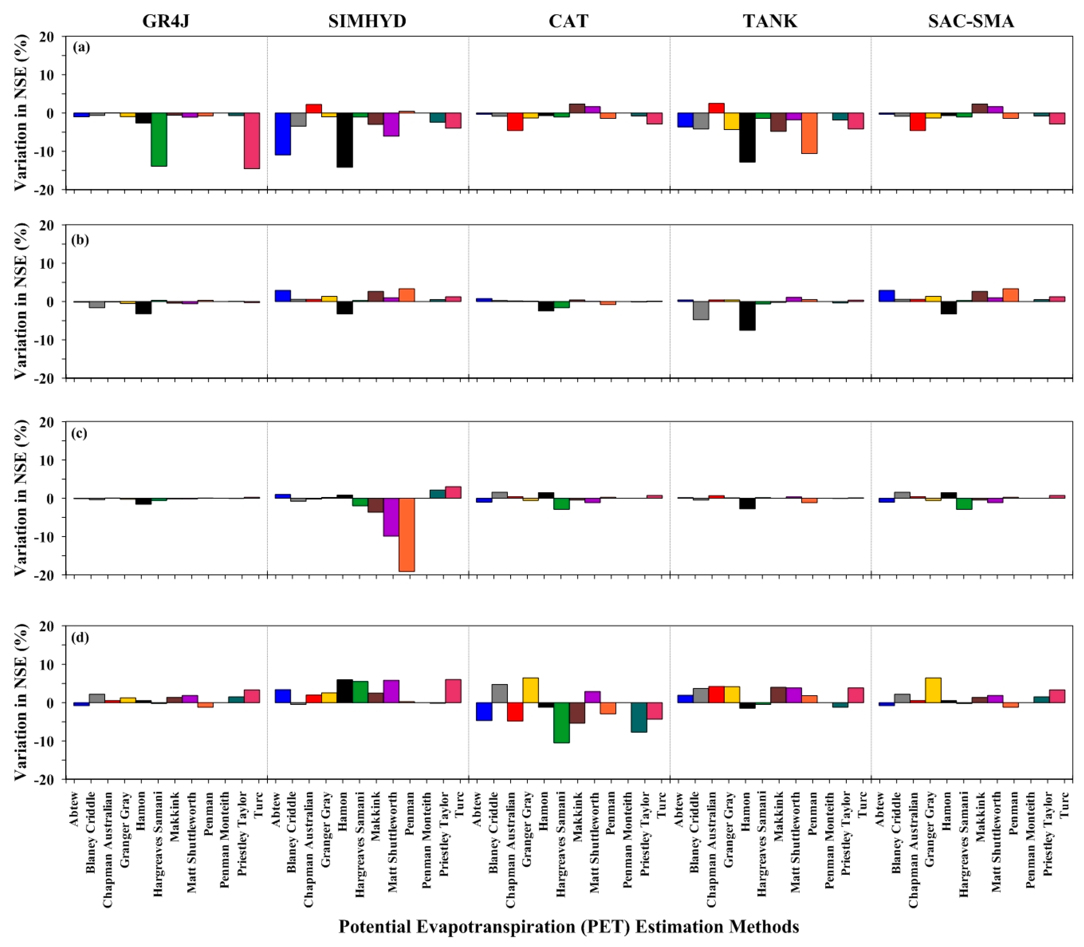
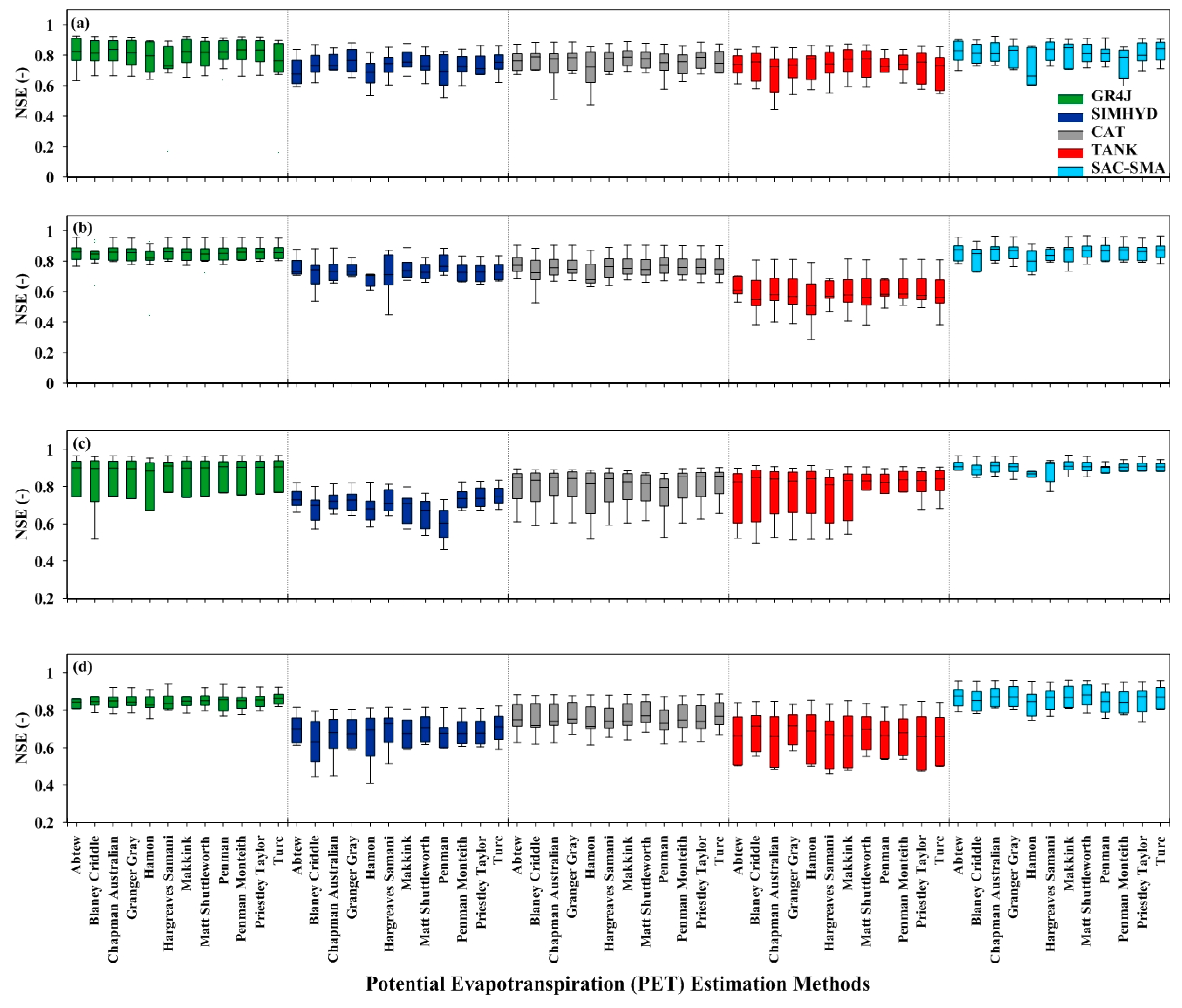
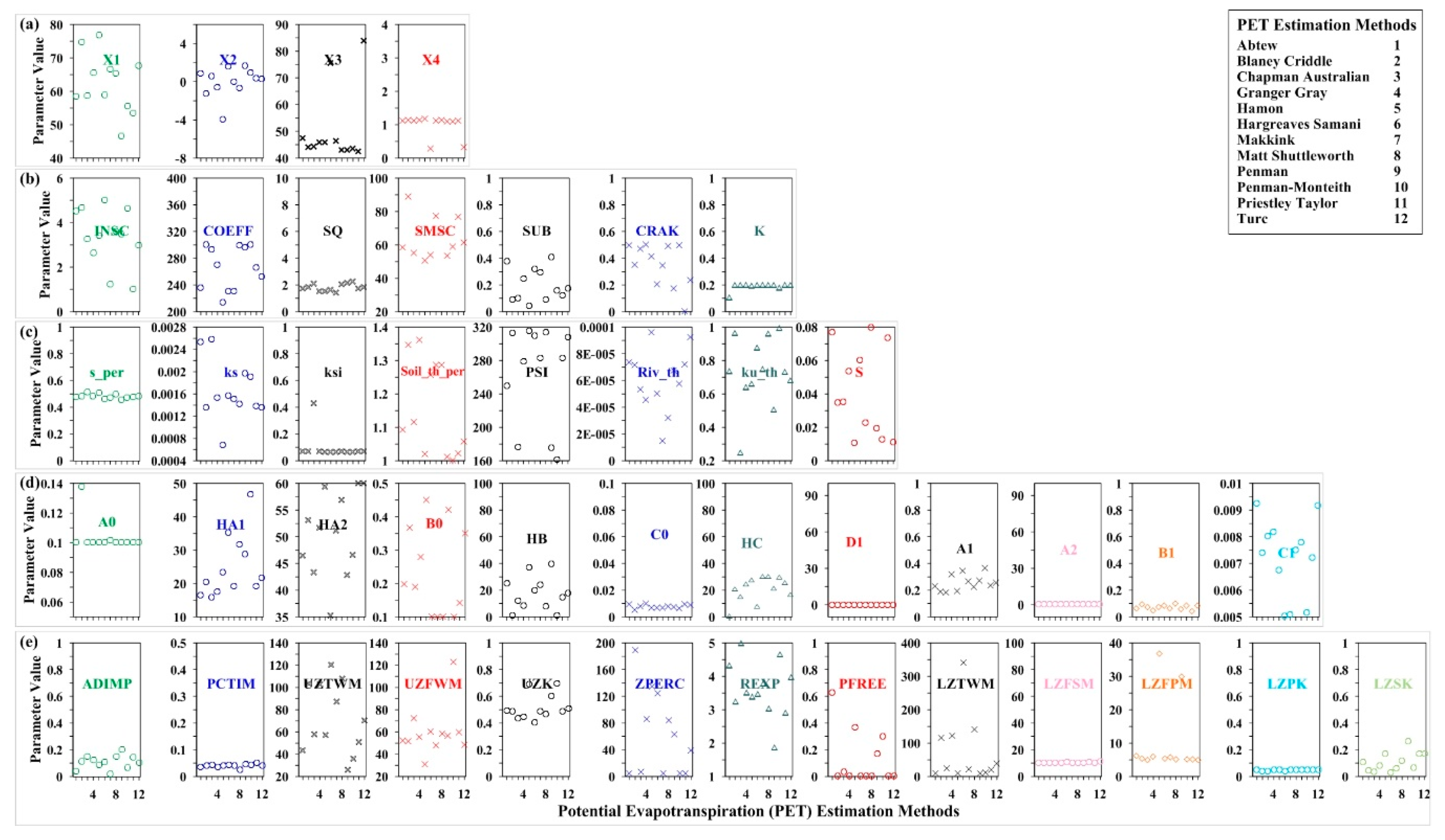
3.3. Effect of PET Complexity on Model Parameters

The GR4J model, the production store (X1), water exchange coefficient (X2), and routing store (X3) parameters were used to adjust the overestimated and underestimated PET values for a better streamflow simulation. The unit hydrograph time base parameter (X4) was only responsible for fixing the lag time and it was insensitive to the 12 different PET input values. However, the three model parameters, X1, X2, and X3 were found to be sensitive to 12 different PET input values, as shown in Figure 9a. The SIMHYD model, the interception store capacity (INSE), maximum infiltration loss (COEFF), and soil moisture store capacity (SMSC) parameters were observed to be sensitive to 12 different PET input values, but the remaining parameters were relatively stable as shown in Figure 9b. The CAT model, wetting front soil suction head (PSI) parameter was sensitive to the 12 different PET inputs values, as shown in Figure 9c, and the remaining parameters were fairly stable in all the tested catchments. The response of the TANK model parameters to the 12 different PET inputs was clearly captured by the vertically arranged water level of the series of tanks, including the height of the runoff outlets of the first (HA1, HA2), second (HB), and third (HC) tanks, as shown in Figure 9d. Similarly, the SAC-SMA model, the upper layer tension water capacity (UZTWM), upper layer free water capacity (UZFWM), lower layer tension water capacity (LZTWM), lower layer supplemental free water capacity (LZFSM), and lower layer primary free water capacity (LZFPM), and the ratio of maximum and minimum percolation rates (ZPERC) parameters were significantly affected by the 12 PET input values, as shown in Figure 9e. The remaining SAC-SMA model parameters were quite stable in all of the tested catchments. The GR4J, SIMHYD, CAT, TANK, and SAC-SMA models’ parameters showed a similar response to the 12 PET input in all the tested catchments and the calibrated parameters were also found to be within the recommended ranges. The five hydrological models’ parameters response to the 12 PET input for the Boryeong catchment is shown in Figure 9.

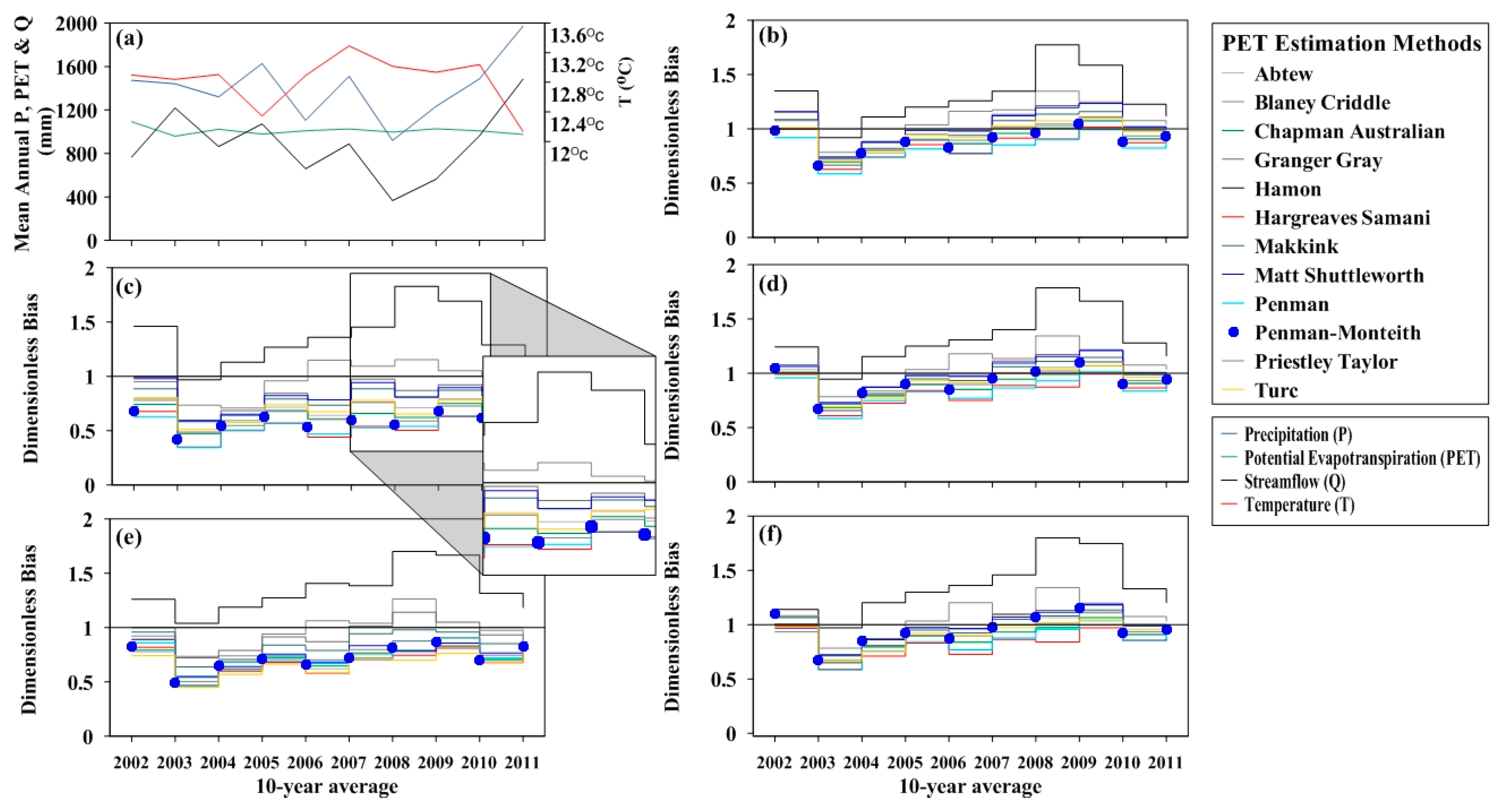
3.4. Effect of PET and Model Structure Complexity on Model Robustness

The three statistical indicators, AIC, BIC, and Ra² values, calculated to compare a model structure also showed similar results with the model performance evaluation index values (NSE, LogNSE, RSR, and KGE). The GR4J, CAT, and SAC-SMA models’ statistical indicator showed a minimum AIC, BIC, and maximum Ra² value in all of the tested catchments, both in the calibration and validation periods. The minimum AIC, BIC, and maximum Ra² value showed that the GR4J, CAT, and SAC-SMA had better model performance for simulating streamflow (Figure 10). However, the SIMHYD and TANK models showed a higher AIC, BIC, and lower Ra² for most of the tested catchments when compared with the GR4J, CAT, and SAC-SMA models’ statistical indicator values. Moreover, the effect of the 12 PET complexity was more captured by the three statistical indicators, and higher AIC, BIC, and lower Ra² values were also observed for the Hamon PET input values, as shown in Figure 10. Similar responses were also observed in all of the tested catchments and Figure 10 shows the AIC, BIC, and Ra² values of four selected catchments for the 12 PET input values in the validation periods.

The PET and model structure complexity effect on model robustness were significantly affected by the low flow and the simulated streamflow was found to be greater than the observed, except the SIMHYD and TANK models. The Dimensionless Bias result also showed a higher water balance error, particularly for extreme hydrological conditions (high and low flow). Similarly, the five hydrological models overestimated the streamflow for the Hamon PET input value and a higher water balance error was observed as shown in Figure 11. The GR4J, CAT, and SAC-SMA models’ behavioral similarities with a relatively lower water balance error were observed (Figure 11) and similar responses were also seen in all of the tested catchments. The SIMHYD and TANK models showed a relatively higher water balance error and a lack of robustness was noticed for normal hydrological conditions, as shown in Figure 10. For a perfectly robust model, flat curves (Dimensionless Bias ≈ 1) and a minor water balance error were expected, but the results that were obtained showed a lack of robustness particularly for average hydrological conditions besides Hamon lack of robustness is observed for low flow conditions. The five hydrological models’ Dimensionless Bias and behavioral similarities to the 12 PET inputs in the Boryeong catchment are shown in Figure 11 and similar responses were also observed in all of the tested catchments.

4. Discussion

Most studies that were conducted in the subject area showed interesting results. The advantages of applying simple models rather than a complex one were first suggested by testing a topography-based model in a small forested catchment in the United States [107]. A similar finding was also obtained when three event-based rainfall-runoff models were applied [108]. Furthermore, Beven [109] suggested the use of three to five parameters to characterize the most dominant physical processes. Recent studies have also shown that complexity does not necessarily enhance the robustness of hydrological models; rather, data quality and hydrological characteristics have more influence on the robustness [7,110,111]. The benefit of reducing the water balance error to enhance conceptual rainfall-runoff models robustness has also been addressed briefly in recent studies [47,48,106].

The GR4J, SIMHYD, CAT, TANK, and SAC-SMA models have increasing levels of complexity. Of these models, the GR4J have the least parameters (four parameters), SIMHYD (seven parameters), CAT (eight parameters), and TANK (12 parameters) are moderate, and the SAC-SMA have several parameters (16 parameters). Similarly, for the 12 PET estimation methods, the data requirements also varied from simple (T) to complex (T, RH, R_S, n, and u). The five hydrological models’ performance was relatively low in the Imha and Andong catchments when compared to the other tested catchments in the validation periods. The Hamon PET estimation method was the only input that clearly showed a decreasing model performance in all of the tested catchments, except for Seolmacheon. This decrease in model performance was likely due to the underestimated values of the Hamon PET estimation method in all of the tested catchments. The better model performance and stable parameters observed in the smallest Seolmacheon experimental catchment were probably related to the size or the availability of high-quality hydro-meteorological data when compared to other study sites. The complexity of the PET estimation method and hydrological model structure did not affect the model performance significantly because of the efficiency of the SCE-UA algorithm to optimize the model parameters for each PET input in the calibration process.

The complexity of the PET inputs had a significant influence on the five hydrological models’ parameters. Particularly, model parameters that are responsible for transforming the PET to AET were found to be sensitive for all of the tested catchments. The GR4J model, X1 parameter is in charge of changing the total PET input value by optimizing the level of production reservoir based on the net rainfall intensity and net evapotranspiration. The X3 parameter variation was mainly caused by the complexity of the PET estimation methods that led to the higher or lower values that affect the routing reservoir. However, the X2 parameter’s identical response to different PET inputs could be an indication of minor groundwater exchange in the tested catchments. The SIMHYD model’s COEFF and SMSC parameters were more sensitive than the INSE parameter. The small variations of the INSE parameters showed the dominance of evapotranspiration from the soil moisture store rather than from the interception store. However, the SMSC parameter variation was due to the SMSC linear relationship with evapotranspiration. The COEFF parameter was affected by the nonlinear relationship with the SMSC parameter in the infiltration estimation process. The sensitivity of these three parameters might help us understand the effect of soil moisture and land use on evaporation. The CAT model PSI parameter sensitivity to the PET input was due to the dependence of the model evapotranspiration on the land use of the 10 tested catchments, which is forest dominated. However, the river and aquifer parameters were not sensitive in all of the tested catchments. In the TANK model, the sensitivity of four of the parameters (HA1, HA2, HB, and HC) to PET inputs was because the model assumption for transforming the water level of each tank to AET was initially based on the availability of water on the sequentially arranged tanks. The other parameters remained insensitive as the output from each tank was transformed to surface, intermediate, and subbase runoff. In the SAC-SMA model, tension water and free water storage parameter sensitivity to PET input was because the AET estimations from the upper and lower water storage were proportional to the magnitude of PET, whereas the sensitivity of the ZPERC parameter was unexpected, as it is responsible for controlling percolation. The unexpected responses of the ZPERC parameters could be related to the problem of finding a unique set of values and over-parameterization, which occurs in most rainfall-runoff models. Similar findings were observed in a previous research work conducted while using the GR4J and TOPMODEL models when considering different PET input scenarios [17].

The results of the three statistical indicators (AIC, BIC, and Ra²) also agreed with the computed model evaluation index values (NSE, LogNSE, RSR, and KGE). The results of the three statistical indicator showed higher AIC, BIC, and lower Ra² values for the Hamon PET estimation method in all of the tested catchments. The lower performance for the Hamon PET input was most likely due to the underestimated value of the PET. The 12 PET estimation methods and five hydrological models’ structure complexity effect were better captured by the three statistical indicators. Although the model complexity comparison criteria (AIC, BIC, and Ra²) results revealed that the GR4J, CAT, and SAC-SMA models had a better capability to simulate streamflow, it would be naive to identify the best hydrological model. The GR4J, CAT, and SAC-SMA models’ behavioral similarities and lower Dimensionless Bias were observed in all of the tested catchments. The five hydrological models lacked robustness, particularly for extreme hydrological conditions (high and low flow) and for the Hamon PET input value, which was observed in all of the tested catchments, except the Seolmacheon. Perrin et al. [7] also discussed the difficulty of identifying the best hydrological model. Furthermore, a previous study conducted on the frequency analysis of hydrological extremes also addressed the limitations and difficulties of completely concluding the superiority of one model for practical applications [46].

5. Conclusions

In this study, the responses of five hydrological models to the 12 PET estimation methods and their effect on model performance, optimized parameters, and robustness were assessed. The GR4J, SIMHYD, CAT, TANK, and SAC-SMA models with increasing levels of complexity were applied over 10 catchments that are located in South Korea. The 10 selected catchments represented the main hydrological characteristics of the Korean Peninsula and have continuous hydro-meteorological data with negligible artificial effects on streamflow. The 10 catchments are mainly covered with forest and sandy loam soil. The 12 PET estimation methods that were used in this study varied from simple to more data demanding. The Hamon PET estimation method was the only input that underestimated the estimated daily PET values in all of the tested catchments except for the Seolmacheon. The SCE-UA algorithm was used to calibrate five hydrological models for the 12 PET inputs when considering four objective functions: NSE, KGE, and RSR. The GR4J, CAT, and SAC-SMA models showed a consistent model performance regardless of the differences in model structure complexity in both the calibration and validation periods. The five hydrological models’ performance were not sensitive to the 12 PET inputs due to the SCE-UA algorithm’s robustness and efficiency. However, the five hydrological models’ parameters in charge of transforming the PET to AET were observed to be sensitive for the PET input values.

The Hamon PET estimation method was the only method that showed decreasing model performance in all of the tested catchments, except for the Seolmacheon. The results of the three statistical indicators (AIC, BIC, and Ra²) captured the PET and hydrological model structure complexity. The model complexity comparison criteria results showed minimum AIC, BIC, and maximum Ra² values for the GR4J, CAT, and SAC-SMA, which is in agreement with the computed model evaluation index values (NSE, RSR and KGE). In addition, the three hydrological models showed lower Dimensionless Bias, and identical behavioral similarities were observed in all of the tested catchments. However, the five hydrological models’ lack of robustness were observed for high and low flow, as well as the Hamon PET input values in all of the tested catchments.

The results of this study revealed the dependence of the model performance and robustness on hydrological conditions (high and low flow) and catchment characteristics, rather than on complexity. The findings of this study will provide a certain level of confidence for hydrologists who work with simple hydrological models and PET estimation methods, particularly in areas with limited hydro-meteorological data, provided that standard datasets are employed.

References

1. Hrachowitz, M.; Clark, M.P. HESS Opinions: The complementary merits of competing modelling philosophies in hydrology. Hydrol. Earth Syst. Sci. 2017, 21, 3953–3973. [Google Scholar] [CrossRef] [Green Version]
2. Brown, C.M.; Lund, J.R.; Cai, X.; Reed, P.M.; Zagona, E.A.; Ostfeld, A.; Hall, J.; Characklis, G.W.; Yu, W.; Brekke, L. The future of water resources systems analysis: Toward a scientific framework for sustainable water management. Water Resour. Res. 2015, 51, 6110–6124. [Google Scholar] [CrossRef] [Green Version]
3. Casadei, S.; Pierleoni, A.; Bellezza, M. Sustainability of Water Withdrawals in the Tiber River Basin (Central Italy). Sustainability 2018, 10, 485. [Google Scholar] [CrossRef]
4. Park, D.; Kim, Y.; Um, M.-J.; Choi, S.-U. Robust Priority for Strategic Environmental Assessment with Incomplete Information Using Multi-Criteria Decision Making Analysis. Sustainability 2015, 7, 10233–10249. [Google Scholar] [CrossRef] [Green Version]
5. Horne, J. Water Information as a Tool to Enhance Sustainable Water Management—The Australian Experience. Water 2015, 7, 2161–2183. [Google Scholar] [CrossRef] [Green Version]
6. Chung, E.-S.; Abdulai, P.J.; Park, H.; Kim, Y.; Ahn, S.R.; Kim, S.J. Multi-Criteria Assessment of Spatial Robust Water Resource Vulnerability Using the TOPSIS Method Coupled with Objective and Subjective Weights in the Han River Basin. Sustainability 2016, 9, 29. [Google Scholar] [CrossRef]
7. Perrin, C.; Michel, C.; Andréassian, V. Does a large number of parameters enhance model performance? Comparative assessment of common catchment model structures on 429 catchments. J. Hydrol. 2001, 242, 275–301. [Google Scholar] [CrossRef]
8. Beck, H.E.; van Dijk, A.I.; de Roo, A.; Dutra, E.; Fink, G.; Orth, R.; Schellekens, J. Global evaluation of runoff from 10 state-of-the-art hydrological models. Hydrol. Earth Syst. Sci. 2017, 21, 2881–2903. [Google Scholar] [CrossRef] [Green Version]
9. Beven, K.J. Rainfall-Runoff Modelling: The Primer, 2nd ed.; Wiley-Blackwell: Chichester, UK; Hoboken, NJ, USA, 2012; ISBN 978-0-47-071459-1. [Google Scholar]
10. Beven, K. How far can we go in distributed hydrological modelling? Hydrol. Earth Syst. Sci. Discuss. 2001, 5, 1–12. [Google Scholar] [CrossRef] [Green Version]
11. Goderniaux, P.; Brouyère, S.; Fowler, H.J.; Blenkinsop, S.; Therrien, R.; Orban, P.; Dassargues, A. Large scale surface–subsurface hydrological model to assess climate change impacts on groundwater reserves. J. Hydrol. 2009, 373, 122–138. [Google Scholar] [CrossRef]
12. Kim, N.W.; Chung, I.M.; Won, Y.S.; Arnold, J.G. Development and application of the integrated SWAT–MODFLOW model. J. Hydrol. 2008, 356, 1–16. [Google Scholar] [CrossRef]
13. Butts, M.B.; Payne, J.T.; Kristensen, M.; Madsen, H. An evaluation of the impact of model structure on hydrological modelling uncertainty for streamflow simulation. J. Hydrol. 2004, 298, 242–266. [Google Scholar] [CrossRef]
14. Bennett, J.C.; Robertson, D.E.; Ward, P.G.D.; Hapuarachchi, H.A.P.; Wang, Q.J. Calibrating hourly rainfall-runoff models with daily forcings for streamflow forecasting applications in meso-scale catchments. Environ. Model. Softw. 2016, 76, 20–36. [Google Scholar] [CrossRef]
15. Perrin, C.; Michel, C.; Andréassian, V. Improvement of a parsimonious model for streamflow simulation. J. Hydrol. 2003, 279, 275–289. [Google Scholar] [CrossRef]
16. Jung, D.; Choi, Y.H.; Kim, J.H. Multiobjective Automatic Parameter Calibration of a Hydrological Model. Water 2017, 9, 187. [Google Scholar] [CrossRef]
17. Andréassian, V.; Perrin, C.; Michel, C. Impact of imperfect potential evapotranspiration knowledge on the efficiency and parameters of watershed models. J. Hydrol. 2004, 286, 19–35. [Google Scholar] [CrossRef]
18. Ficchì, A.; Perrin, C.; Andréassian, V. Impact of temporal resolution of inputs on hydrological model performance: An analysis based on 2400 flood events. J. Hydrol. 2016, 538, 454–470. [Google Scholar] [CrossRef]
19. Oudin, L.; Michel, C.; Anctil, F. Which potential evapotranspiration input for a lumped rainfall-runoff model? Part 1—Can rainfall-runoff models effectively handle detailed potential evapotranspiration inputs? J. Hydrol. 2005, 303, 275–289. [Google Scholar] [CrossRef]
20. Oudin, L.; Hervieu, F.; Michel, C.; Perrin, C.; Andréassian, V.; Anctil, F.; Loumagne, C. Which potential evapotranspiration input for a lumped rainfall-runoff model? Part 2—Towards a simple and efficient potential evapotranspiration model for rainfall–runoff modelling. J. Hydrol. 2005, 303, 290–306. [Google Scholar] [CrossRef]
21. Knipper, K.; Hogue, T.; Scott, R.; Franz, K. Evapotranspiration Estimates Derived Using Multi-Platform Remote Sensing in a Semiarid Region. Remote Sens. 2017, 9, 184. [Google Scholar] [CrossRef]
22. Harrigan, S.; Berghuijs, W. The Mystery of Evaporation. Streams of Thought. Young Hydrol. Soc. 2016, 10. [Google Scholar] [CrossRef]
23. Guo, D.; Westra, S.; Maier, H.R. An R package for modelling actual, potential and reference evapotranspiration. Environ. Model. Softw. 2016, 78, 216–224. [Google Scholar] [CrossRef]
24. Parmele, L.H. Errors in output of hydrologic models due to errors in input potential evapotranspiration. Water Resour. Res. 1972, 8, 348–359. [Google Scholar] [CrossRef]
25. Nandakumar, N.; Mein, R.G. Uncertainty in rainfall-runoff model simulations and the implications for predicting the hydrologic effects of land-use change. J. Hydrol. 1997, 192, 211–232. [Google Scholar] [CrossRef]
26. Paturel, J.E.; Servat, E.; Vassiliadis, A. Sensitivity of conceptual rainfall-runoff algorithms to errors in input data—Case of the GR2M model. J. Hydrol. 1995, 168, 111–125. [Google Scholar] [CrossRef]
27. Xu, C.-Y.; Vandewiele, G.L. Sensitivity of monthly rainfall-runoff models to input errors and data length. Hydrol. Sci. J. 1994, 39, 157–176. [Google Scholar] [CrossRef] [Green Version]
28. Xu, C.; Tunemar, L.; Chen, Y.D.; Singh, V.P. Evaluation of seasonal and spatial variations of lumped water balance model sensitivity to precipitation data errors. J. Hydrol. 2006, 324, 80–93. [Google Scholar] [CrossRef]
29. Barella-Ortiz, A.; Polcher, J.; Tuzet, A.; Laval, K. Potential evaporation estimation through an unstressed surface-energy balance and its sensitivity to climate change. Hydrol. Earth Syst. Sci. 2013, 17, 4625–4639. [Google Scholar] [CrossRef] [Green Version]
30. McVicar, T.R.; Roderick, M.L.; Donohue, R.J.; Li, L.T.; Van Niel, T.G.; Thomas, A.; Grieser, J.; Jhajharia, D.; Himri, Y.; Mahowald, N.M.; et al. Global review and synthesis of trends in observed terrestrial near-surface wind speeds: Implications for evaporation. J. Hydrol. 2012, 416–417, 182–205. [Google Scholar] [CrossRef]
31. Andersson, L. Improvements of runoff models what way to go? Hydrol. Res. 1992, 23, 315–332. [Google Scholar] [CrossRef]
32. Lindroth, A. Potential Evaporation—A Matter of Definition: A Comment on ‘Improvements of Runoff Models—What Way to Go’? Hydrol. Res. 1993, 24, 359–364. [Google Scholar] [CrossRef]
33. Morton, F.I. Evaporation research—A critical review and its lessons for the environmental sciences. Crit. Rev. Environ. Sci. Technol. 1994, 24, 237–280. [Google Scholar] [CrossRef]
34. Evans, J.P. Improving the characteristics of streamflow modeled by regional climate models. J. Hydrol. 2003, 284, 211–227. [Google Scholar] [CrossRef]
35. Oudin, L.; Andréassian, V.; Perrin, C.; Anctil, F. Locating the sources of low-pass behavior within rainfall-runoff models: Low-pass behavior of rainfall-runoff models. Water Resour. Res. 2004, 40. [Google Scholar] [CrossRef]
36. Oudin, L.; Perrin, C.; Mathevet, T.; Andréassian, V.; Michel, C. Impact of biased and randomly corrupted inputs on the efficiency and the parameters of watershed models. J. Hydrol. 2006, 320, 62–83. [Google Scholar] [CrossRef]
37. Nash, J.E.; Sutcliffe, J.V. River flow forecasting through conceptual models. Part I—A discussion of principles. J. Hydrol. 1970, 10, 282–290. [Google Scholar] [CrossRef]
38. Beven, K.; Binley, A. GLUE: 20 years on. Hydrol. Process. 2014, 28, 5897–5918. [Google Scholar] [CrossRef]
39. Moussa, R.; Chahinian, N. Comparison of different multi-objective calibration criteria using a conceptual rainfall-runoff model of flood events. Hydrol. Earth Syst. Sci. 2009, 13, 519–535. [Google Scholar] [CrossRef] [Green Version]
40. Moriasi, D.N.; Arnold, J.G.; Van Liew, M.W.; Bingner, R.L.; Harmel, R.D.; Veith, T.L. Model evaluation guidelines for systematic quantification of accuracy in watershed simulations. Trans. ASABE 2007, 50, 885–900. [Google Scholar] [CrossRef]
41. Gupta, H.V.; Kling, H.; Yilmaz, K.K.; Martinez, G.F. Decomposition of the mean squared error and NSE performance criteria: Implications for improving hydrological modelling. J. Hydrol. 2009, 377, 80–91. [Google Scholar] [CrossRef] [Green Version]
42. Clark, M.P.; Slater, A.G.; Rupp, D.E.; Woods, R.A.; Vrugt, J.A.; Gupta, H.V.; Wagener, T.; Hay, L.E. Framework for Understanding Structural Errors (FUSE): A modular framework to diagnose differences between hydrological models. Water Resour. Res. 2008, 44, W00B02. [Google Scholar] [CrossRef]
43. Akaike, H. A new look at the statistical model identification. IEEE Trans. Autom. Control 1974, 19, 716–723. [Google Scholar] [CrossRef]
44. Schwarz, G. Estimating the Dimension of a Model. Ann. Stat. 1978, 6, 461–464. [Google Scholar] [CrossRef]
45. Qi, M.; Zhang, G.P. An investigation of model selection criteria for neural network time series forecasting. Eur. J. Oper. Res. 2001, 132, 666–680. [Google Scholar] [CrossRef]
46. Laio, F.; Di Baldassarre, G.; Montanari, A. Model selection techniques for the frequency analysis of hydrological extremes. Water Resour. Res. 2009, 45, W07416. [Google Scholar] [CrossRef]
47. Merz, R.; Parajka, J.; Blöschl, G. Time stability of catchment model parameters: Implications for climate impact analyses. Water Resour. Res. 2011, 47, W02531. [Google Scholar] [CrossRef]
48. Coron, L.; Andréassian, V.; Perrin, C.; Bourqui, M.; Hendrickx, F. On the lack of robustness of hydrologic models regarding water balance simulation: A diagnostic approach applied to three models of increasing complexity on 20 mountainous catchments. Hydrol. Earth Syst. Sci. 2014, 18, 727–746. [Google Scholar] [CrossRef]
49. Duan, Q.; Sorooshian, S.; Gupta, V.K. Optimal use of the SCE-UA global optimization method for calibrating watershed models. J. Hydrol. 1994, 158, 265–284. [Google Scholar] [CrossRef] [Green Version]
50. Ajami, N.K.; Gupta, H.; Wagener, T.; Sorooshian, S. Calibration of a semi-distributed hydrologic model for streamflow estimation along a river system. J. Hydrol. 2004, 298, 112–135. [Google Scholar] [CrossRef]
51. Madsen, H. Automatic calibration of a conceptual rainfall–runoff model using multiple objectives. J. Hydrol. 2000, 235, 276–288. [Google Scholar] [CrossRef]
52. Roy, T.; Gupta, H.V.; Serrat-Capdevila, A.; Valdes, J.B. Using satellite-based evapotranspiration estimates to improve the structure of a simple conceptual rainfall–runoff model. Hydrol. Earth Syst. Sci. 2017, 21, 879–896. [Google Scholar] [CrossRef] [Green Version]
53. McMahon, T.A.; Peel, M.C.; Lowe, L.; Srikanthan, R.; McVicar, T.R. Estimating actual, potential, reference crop and pan evaporation using standard meteorological data: A pragmatic synthesis. Hydrol. Earth Syst. Sci. 2013, 17, 1331–1363. [Google Scholar] [CrossRef]
54. Xu, C.-Y.; Singh, V.P. Cross Comparison of Empirical Equations for Calculating Potential Evapotranspiration with Data from Switzerland. Water Resour. Manag. 2002, 16, 197–219. [Google Scholar] [CrossRef]
55. Brutsaert, W. Evaporation into the Atmosphere: Theory, History and Applications; Springer: Dordrecht, The Netherlands, 1982; ISBN 978-9-40-171497-6. [Google Scholar]
56. Zhao, L.; Xia, J.; Xu, C.; Wang, Z.; Sobkowiak, L.; Long, C. Evapotranspiration estimation methods in hydrological models. J. Geogr. Sci. 2013, 23, 359–369. [Google Scholar] [CrossRef]
57. García Hernández, J.; Claude, A.; Paredes Arquiola, J.; Roquier, B.; Boillat, J.-L. Integrated flood forecasting and management system in a complex catchment area in the Alps—Implementation of the MINERVE project in the Canton of Valais. In Special Session on Swiss Competences in River Engineering and Restoration, Proceedings of the River Flow 2014, Lausanne, Switzerland, 3–5 September 2014; EPFL: Leiden, Switzerland, 2014; pp. 87–97. [Google Scholar]
58. Demirel, M.C.; Booij, M.J.; Hoekstra, A.Y. The skill of seasonal ensemble low-flow forecasts in the Moselle River for three different hydrological models. Hydrol. Earth Syst. Sci. 2015, 19, 275–291. [Google Scholar] [CrossRef] [Green Version]
59. Kim, D.; Jung, I.W.; Chun, J.A. A comparative assessment of rainfall–runoff modelling against regional flow duration curves for ungauged catchments. Hydrol. Earth Syst. Sci. 2017, 21, 5647–5661. [Google Scholar] [CrossRef] [Green Version]
60. Nepal, S.; Chen, J.; Penton, D.J.; Neumann, L.E.; Zheng, H.; Wahid, S. Spatial GR4J conceptualization of the Tamor glaciated alpine catchment in Eastern Nepal: Evaluation of GR4JSG against streamflow and MODIS snow extent: Hydrological Modelling in Tamor Catchment. Hydrol. Process. 2017, 31, 51–68. [Google Scholar] [CrossRef]
61. Velázquez, J.A.; Anctil, F.; Ramos, M.H.; Perrin, C. Can a multi-model approach improve hydrological ensemble forecasting? A study on 29 French catchments using 16 hydrological model structures. Adv. Geosci. 2011, 29, 33–42. [Google Scholar] [CrossRef] [Green Version]
62. Ajmal, M.; Khan, T.A.; Kim, T.-W. A CN-Based Ensembled Hydrological Model for Enhanced Watershed Runoff Prediction. Water 2016, 8, 20. [Google Scholar] [CrossRef]
63. Tian, Y.; Booij, M.J.; Xu, Y.-P. Uncertainty in high and low flows due to model structure and parameter errors. Stoch. Environ. Res. Risk Assess. 2014, 28, 319–332. [Google Scholar] [CrossRef]
64. Porter, J.W.; McMahon, T.A. Application of a catchment model in southeastern Australia. J. Hydrol. 1975, 24, 121–134. [Google Scholar] [CrossRef]
65. Chiew, F.H.S.; Peel, M.C.; Western, A.W. Application and testing of the simple rainfall-runoff model SIMHYD. In Mathematical Models of Small Watershed Hydrology and Applications; Singh, V.P., Frevert, D.K., Eds.; Water Resources Publications: Littleton, CO, USA, 2002; pp. 335–367. [Google Scholar]
66. Chiew, F.H.S.; Kirono, D.G.C.; Kent, D.M.; Frost, A.J.; Charles, S.P.; Timbal, B.; Nguyen, K.C.; Fu, G. Comparison of runoff modelled using rainfall from different downscaling methods for historical and future climates. J. Hydrol. 2010, 387, 10–23. [Google Scholar] [CrossRef]
67. Li, C.Z.; Zhang, L.; Wang, H.; Zhang, Y.Q.; Yu, F.L.; Yan, D.H. The transferability of hydrological models under nonstationary climatic conditions. Hydrol. Earth Syst. Sci. 2012, 16, 1239–1254. [Google Scholar] [CrossRef] [Green Version]
68. Li, H.; Zhang, Y. Regionalising rainfall-runoff modelling for predicting daily runoff: Comparing gridded spatial proximity and gridded integrated similarity approaches against their lumped counterparts. J. Hydrol. 2017, 550, 279–293. [Google Scholar] [CrossRef]
69. Vaze, J.; Post, D.A.; Chiew, F.H.S.; Perraud, J.-M.; Teng, J.; Viney, N.R. Conceptual Rainfall–Runoff Model Performance with Different Spatial Rainfall Inputs. J. Hydrometeorol. 2011, 12, 1100–1112. [Google Scholar] [CrossRef]
70. Yu, B.; Zhu, Z. A comparative assessment of AWBM and SimHyd for forested watersheds. Hydrol. Sci. J. 2015, 60, 1200–1212. [Google Scholar] [CrossRef]
71. Peel, M.C.; Chiew, F.H.; Western, A.W.; McMahon, T.A. Extension of Unimpaired Monthly Streamflow Data and Regionalisation of Parameter Values to Estimate Streamflow in Ungauged Catchments; Australian Natural Resources Atlas: Melbourne, Australia, 2000. [Google Scholar]
72. Kim, H.-J.; Jang, C.-H. Catchment Hydrologic Cycle Assessment Tool—A User Guide; Korea Institute of Civil Engineering and Building Technology: Goyang, Korea, 2017. [Google Scholar]
73. Miller, J.D.; Kim, H.; Kjeldsen, T.R.; Packman, J.; Grebby, S.; Dearden, R. Assessing the impact of urbanization on storm runoff in a peri-urban catchment using historical change in impervious cover. J. Hydrol. 2014, 515, 59–70. [Google Scholar] [CrossRef] [Green Version]
74. Kim, H.-J.; Jang, C.-H.; Noh, S.-J. Development and application of the catchment hydrologic cycle assessment tool considering urbanization (I)-Model development. J. Korea Water Resour. Assoc. 2012, 45, 203–215. [Google Scholar] [CrossRef]
75. Green, W.H.; Ampt, G.A. Studies on Soil Phyics. J. Agric. Sci. 1911, 4, 1–24. [Google Scholar] [CrossRef]
76. Jang, C.H.; Kim, H.J.; Ahn, S.R.; Kim, S.J. Assessment of hydrological changes in a river basin as affected by climate change and water management practices, by using the cat model. Irrig. Drain. 2016, 65, 26–35. [Google Scholar] [CrossRef]
77. Jang, C.-H.; Kim, H.-J.; Kim, J.-T. Prediction of Reservoir Water Level using CAT. J. Korean Soc. Agric. Eng. 2012, 54, 27–38. [Google Scholar] [CrossRef] [Green Version]
78. Choi, S.; Jang, C.; Kim, H. Analysis of Short-term Runoff Characteristics of CAT-PEST Connected Model using Different Infiltration Analysis Methods. J. Korea Acad. Ind. Coop. Soc. 2016, 17, 26–41. [Google Scholar] [CrossRef]
79. Hwang, S.; Kang, M.-S. Evaluation of the CAT Model in hydrological simulation for a small watershed. In Proceedings of the 2012 ASABE Annual International Meeting, Dallas, TX, USA, 29 July–1 August 2012; American Society of Agricultural and Biological Engineers: St. Joseph, MI, USA, 2012; p. 1. [Google Scholar]
80. Sugawara, M. Automatic calibration of the tank model/L’étalonnage automatique d’un modèle à cisterne. Hydrol. Sci. Bull. 1979, 24, 375–388. [Google Scholar] [CrossRef]
81. Chadalawada, J.; Havlicek, V.; Babovic, V. A Genetic Programming Approach to System Identification of Rainfall-Runoff Models. Water Resour. Manag. 2017, 31, 3975–3992. [Google Scholar] [CrossRef]
82. Sugawara, M. Tank model. In Computer Models of Watershed Hydrology; Singh, V.P., Ed.; Water Resources Publications: Littleton, CO, USA, 1995; ISBN 0-918334-91-8. [Google Scholar]
83. Lee, Y.H.; Singh, V.P. Tank Model for Sediment Yield. Water Resour. Manag. 2005, 19, 349–362. [Google Scholar] [CrossRef]
84. Sung, Y.-K.; Kim, S.-H.; Kim, H.-J.; Kim, N.-W. The Applicability Study of SYMHYD and TANK Model Using Different Type of Objective Functions and Optimization Methods. J. Korea Water Resour. Assoc. 2004, 37, 121–131. [Google Scholar] [CrossRef]
85. Yokoo, Y.; Chiba, T.; Shikano, Y.; Leong, C. Identifying dominant runoff mechanisms and their lumped modeling: A data-based modeling approach. Hydrol. Res. Lett. 2017, 11, 128–133. [Google Scholar] [CrossRef]
86. Song, J.-H.; Her, Y.; Park, J.; Lee, K.-D.; Kang, M.-S. Simulink Implementation of a Hydrologic Model: A Tank Model Case Study. Water 2017, 9, 639. [Google Scholar] [CrossRef]
87. Chen, R.-S.; Pi, L.-C.; Hsieh, C.-C. Application of Parameter Optimization Method for Calibrating Tank Model1. J. Am. Water Resour. Assoc. 2005, 41, 389–402. [Google Scholar] [CrossRef]
88. Burnash, R.J.C. The NWS river forecast system-catchment modeling. In Computer Models of Watershed Hydrology; Singh, V.P., Ed.; Water Resources Publications: Littleton, CO, USA, 1995; ISBN 0-918334-91-8. [Google Scholar]
89. Wright, A.J.; Walker, J.P.; Pauwels, V.R.N. Estimating rainfall time series and model parameter distributions using model data reduction and inversion techniques. Water Resour. Res. 2017, 53, 6407–6424. [Google Scholar] [CrossRef]
90. Bowman, A.L.; Franz, K.J.; Hogue, T.S. Case Studies of a MODIS-Based Potential Evapotranspiration Input to the Sacramento Soil Moisture Accounting Model. J. Hydrometeorol. 2016, 18, 151–158. [Google Scholar] [CrossRef]
91. Heřmanovský, M.; Havlíček, V.; Hanel, M.; Pech, P. Regionalization of runoff models derived by genetic programming. J. Hydrol. 2017, 547, 544–556. [Google Scholar] [CrossRef]
92. Huang, C.; Newman, A.J.; Clark, M.P.; Wood, A.W.; Zheng, X. Evaluation of snow data assimilation using the ensemble Kalman filter for seasonal streamflow prediction in the western United States. Hydrol. Earth Syst. Sci. 2017, 21, 635–650. [Google Scholar] [CrossRef]
93. Katsanou, K.; Lambrakis, N. Modeling the Hellenic karst catchments with the Sacramento Soil Moisture Accounting model. Hydrogeol. J. 2017, 25, 757–769. [Google Scholar] [CrossRef]
94. Shin, M.-J.; Guillaume, J.H.A.; Croke, B.F.W.; Jakeman, A.J. Addressing ten questions about conceptual rainfall–runoff models with global sensitivity analyses in R. J. Hydrol. 2013, 503, 135–152. [Google Scholar] [CrossRef]
95. Vrugt, J.A.; Gupta, H.V.; Dekker, S.C.; Sorooshian, S.; Wagener, T.; Bouten, W. Application of stochastic parameter optimization to the Sacramento Soil Moisture Accounting model. J. Hydrol. 2006, 325, 288–307. [Google Scholar] [CrossRef]
96. Anderson, R.M.; Koren, V.I.; Reed, S.M. Using SSURGO data to improve Sacramento Model a priori parameter estimates. J. Hydrol. 2006, 320, 103–116. [Google Scholar] [CrossRef]
97. Khu, S.-T.; Werner, M.G. Reduction of Monte-Carlo simulation runs for uncertainty estimation in hydrological modelling. Hydrol. Earth Syst. Sci. Discuss. 2003, 7, 680–692. [Google Scholar] [CrossRef] [Green Version]
98. Lee, S.; Kang, T. Analysis of Constrained Optimization Problems by the SCE-UA with an Adaptive Penalty Function. J. Comput. Civ. Eng. 2016, 30, 04015035. [Google Scholar] [CrossRef]
99. Van Griensven, A.; Meixner, T.; Grunwald, S.; Bishop, T.; Diluzio, M.; Srinivasan, R. A global sensitivity analysis tool for the parameters of multi-variable catchment models. J. Hydrol. 2006, 324, 10–23. [Google Scholar] [CrossRef]
100. Rosenbrock, H. An automatic method for finding the greatest or least value of a function. Comput. J. 1960, 3, 175–184. [Google Scholar] [CrossRef]
101. Liu, X.; Yang, T.; Hsu, K.; Liu, C.; Sorooshian, S. Evaluating the streamflow simulation capability of PERSIANN-CDR daily rainfall products in two river basins on the Tibetan Plateau. Hydrol. Earth Syst. Sci. 2017, 21, 169–181. [Google Scholar] [CrossRef] [Green Version]
102. Kim, H.; Kim, S.; Shin, H.; Heo, J.-H. Appropriate model selection methods for nonstationary generalized extreme value models. J. Hydrol. 2017, 547, 557–574. [Google Scholar] [CrossRef]
103. Gaganis, P.; Smith, L. A Bayesian Approach to the quantification of the effect of model error on the predictions of groundwater models. Water Resour. Res. 2001, 37, 2309–2322. [Google Scholar] [CrossRef] [Green Version]
104. Kamruzzaman, M.; Shahriar, M.S.; Beecham, S. Assessment of Short Term Rainfall and Stream Flows in South Australia. Water 2014, 6, 3528–3544. [Google Scholar] [CrossRef] [Green Version]
105. Wilby, R.L.; Abrahart, R.J.; Dawson, C.W. Detection of conceptual model rainfall-runoff processes inside an artificial neural network. Hydrol. Sci. J. 2003, 48, 163–181. [Google Scholar] [CrossRef]
106. Coron, L.; Andréassian, V.; Perrin, C.; Lerat, J.; Vaze, J.; Bourqui, M.; Hendrickx, F. Crash testing hydrological models in contrasted climate conditions: An experiment on 216 Australian catchments. Water Resour. Res. 2012, 48, W05552. [Google Scholar] [CrossRef]
107. Hornberger, G.M.; Beven, K.J.; Cosby, B.J.; Sappington, D.E. Shenandoah Watershed Study: Calibration of a Topography-Based, Variable Contributing Area Hydrological Model to a Small Forested Catchment. Water Resour. Res. 1985, 21, 1841–1850. [Google Scholar] [CrossRef]
108. Loague, K.M.; Freeze, R.A. A Comparison of Rainfall-Runoff Modeling Techniques on Small Upland Catchments. Water Resour. Res. 1985, 21, 229–248. [Google Scholar] [CrossRef]
109. Beven, K. Changing ideas in hydrology -The case of physically-based models. J. Hydrol. 1989, 105, 157–172. [Google Scholar] [CrossRef]
110. Orth, R.; Staudinger, M.; Seneviratne, S.I.; Seibert, J.; Zappa, M. Does model performance improve with complexity? A case study with three hydrological models. J. Hydrol. 2015, 523, 147–159. [Google Scholar] [CrossRef] [Green Version]
111. Gan, T.Y.; Dlamini, E.M.; Biftu, G.F. Effects of model complexity and structure, data quality, and objective functions on hydrologic modeling. J. Hydrol. 1997, 192, 81–103. [Google Scholar] [CrossRef]
112. Abtew, W. Evapotranspiration Measurements and Modeling for Three Wetland Systems in South Florida1. J. Am. Water Resour. Assoc. 1996, 32, 465–473. [Google Scholar] [CrossRef]
113. Allen, R.G.; Pruitt, W.O. Rational Use of the FAO Blaney-Criddle Formula. J. Irrig. Drain. Eng. 1986, 112, 139–155. [Google Scholar] [CrossRef]
114. Chapman, T.G. Estimation of evaporation in rainfall-runoff models. In Proceedings of the MODSIM 2003 International Congress on Modelling and Simulation, Townsville, Australia, 14–17 July 2003; Volume 1, pp. 148–153. [Google Scholar]
115. Granger, R.J.; Gray, D.M. Evaporation from natural nonsaturated surfaces. J. Hydrol. 1989, 111, 21–29. [Google Scholar] [CrossRef]
116. Hamon, W.R. Estimating Potential Evapotranspiration. J. Hydraul. Div. 1961, 87, 107–120. [Google Scholar]
117. Hargreaves, G.H.; Samani, Z.A. Reference crop evapotranspiration from temperature. Appl. Eng. Agric. 1985, 1, 96–99. [Google Scholar] [CrossRef]
118. De Bruin, H.A.R.; Lablans, W.N. Reference crop evapotranspiration determined with a modified Makkink equation. Hydrol. Process. 1998, 12, 1053–1062. [Google Scholar] [CrossRef]
119. Shuttleworth, W.J.; Wallace, J.S. Calculating the water requirements of irrigated crops in Australia using the Matt-Shuttleworth approach. Trans. ASABE 2009, 52, 1895–1906. [Google Scholar] [CrossRef]
120. Penman, H.L. Natural evaporation from open water, bare soil and grass. Proc. R. Soc. Lond. A 1948, 193, 120–145. [Google Scholar] [CrossRef]
121. Allen, R.G.; Pereira, L.S.; Raes, D.; Smith, M. FAO Irrigation and Drainage Paper No. 56; Food and Agriculture Organization of the United Nations: Rome, Italy, 1998; Volume 56, pp. 97–156. [Google Scholar]
122. Priestley, C.H.B.; Taylor, R.J. On the Assessment of Surface Heat Flux and Evaporation Using Large-Scale Parameters. Mon. Weather Rev. 1972, 100, 81–92. [Google Scholar] [CrossRef] [Green Version]
123. Turc, L. Estimation of irrigation water requirements, potential evapotranspiration: A simple climatic formula evolved up to date. Ann. Agron. 1961, 12, 13–49. [Google Scholar]
Figure 1. Location of the 10 gauged catchments, major rivers, and streamflow gauging stations.
Sustainability 10 02837 g001
Figure 2. Land use and the soil texture map of the 10 gauged catchments. (a) Land use and (b) Soil texture.
Sustainability 10 02837 g002
Figure 3. Daily Potential Evapotranspiration (PET). (a) Daily PET of Seolmacheon, Boryeong, Kyeongan, Seomjingang, and Yongdam catchments (b) Daily PET of Juam, Imha, Andong, Soyanggang, and Chungju catchments.
Sustainability 10 02837 g003
Figure 4. The performances of the five hydrological models for the 12 Potential Evapotranspiration (PET) input values in the calibration periods. (a) Nash-Sutcliffe Efficiency (NSE); (b) Logarithmic Nash-Sutcliffe Efficiency (LogNSE); (c) Ratio of the root mean square error to the standard deviation of measured data (RSR); and, (d) Kling-Gupta Efficiency (KGE) corresponding to the catchment No. 1–10. The vertical axis corresponds to the model performances of the 12 PET inputs.
Sustainability 10 02837 g004
Figure 5. The performances of the five hydrological models for the 12 Potential Evapotranspiration (PET) input values in the validation periods. (a) Nash-Sutcliffe Efficiency (NSE); (b) Logarithmic Nash-Sutcliffe Efficiency (LogNSE); (c) Ratio of the root mean square error to the standard deviation of measured data (RSR); and, (d) Kling-Gupta Efficiency (KGE) corresponding to the catchment No. 1–10. The vertical axis corresponds to the model performances of the 12 PET inputs.
Sustainability 10 02837 g005
Figure 6. The five hydrological models’ performance percentage variations calculated considering the Penman-Monteith PET input Nash-Sutcliffe Efficiency (NSE) index values as a benchmark for the validation periods. (a) Boryeong; (b) Seomjingang; (c) Soyanggang; and, (d) Chungju catchments.
Sustainability 10 02837 g006
Figure 7. Scatterplot of the five hydrological models’ performance (Nash-Sutcliffe Efficiency (NSE)) for the Penman-Monteith Potential Evapotranspiration (PET) input. (a) Boryeong; (b) Seomjingang; (c) Soyanggang; and, (d) Chungju catchments.
Sustainability 10 02837 g007
Figure 8. Five hydrological models‘ performance (Nash-Sutcliffe Efficiency (NSE)) for the 12 PET inputs. (a) Boryeong; (b) Seomjingang; (c) Soyanggang; and, (d) Chungju catchments.
Sustainability 10 02837 g008
Figure 9. Five hydrological models’ parameters response to the 12 PET input for the Boryeong catchment. (a) Génie Rural à 4 paramètres Journalier (GR4J); (b) Simplified Hydrolog (SIMHYD); (c) Catchment Hydrological Cycle Assessment Tool (CAT); (d) TANK, and (e) Sacramento Soil Moisture Accounting (SAC-SMA). The letters correspond to the five hydrological models’ parameters.
Sustainability 10 02837 g009
Figure 10. Five hydrological models’ statistical indicator values for the 12 PET inputs in the validation periods. (a) Boryeong; (b) Seomjingang; (c) Soyanggang; and, (d) Chungju catchments. The black color is the Akaike Information Criterion (AIC), the green color is the Bayesian Information Criterion (BIC), and the blue black color is the Adjusted R-square (Ra2).
Sustainability 10 02837 g010
Figure 11. Five hydrological models’ Dimensionless Bias and behavioral similarities for the 12 PET inputs values in the Boryeong catchment. (a) Hydro-meteorological data; (b) GR4J; (c) SIMHYD; (d) CAT; (e) TANK; and, (f) SAC-SMA models.
Sustainability 10 02837 g011