An Introduction to the Hyperspace of Hargreaves-Samani Reference Evapotranspiration


1
Civil Engineering Department, University of Minho, Azurem Campus, 4800-058 Guimarães, Portugal
2
Department of Mathematics and Centre of Physics UM-UP, University of Minho, 4710-057 Braga, Portugal
3
Blackland Research and Extension Center, Texas A&M University, Temple, TX 76502, USA
*
Author to whom correspondence should be addressed.
Sustainability 2018, 10(11), 4277; https://doi.org/10.3390/su10114277
Submission received: 26 August 2018
/
Revised: 8 November 2018
/
Accepted: 16 November 2018
/
Published: 19 November 2018
(This article belongs to the Special Issue Watershed Processes under Changing Climate)
Abstract
:Climate change has been shown to directly influence evapotranspiration, which is one of the crucial watershed processes. The common approach to its calculation is via mathematical equations, such as 1985 Hargreaves-Samani (HS85). It computes reference evapotranspiration (ETo) through three climatic variables and one constant: RA (extra-terrestrial radiation), TC (mean temperature), TR (temperature range) and KR (empirical coefficient). To make HS85 more accurate, one of its authors proposed an equation for KR as a function of TR in 2000 (HS00). Both models are 4D and their internal behaviours are difficult to understand, hence, the data driven applications prevalent among experts and managers. In this study, we introduce an innovative research by trying to respond to two questions. What are the relationships between TC and TR? What are the internal patterns of HS hyperspace (4D domain) and the changes in ETo possibilities of the two models? In the proposed approach, thresholds for the four variables are utilized to cover majority of the agroclimatic situations in the world and the hyperspace is discretized with more than 50,000 calculation nodes. The ETo results show that under various climatic conditions, the behaviour of HS is nonlinear (more for HS00) leading to an increased uncertainty particularly for data driven applications. TC and TR show patterns useful for regions with less data.
1. Introduction
National Aeronautics and Space Administration (NASA) & National Oceanic and Atmospheric Administration (NOAA) of the United States confirmed that 2016 was the hottest year on record globally [1]. The World Economic Forum in 2015 [2] reported that among many global issues facing humanity, the number one societal impact is water crises. On the other hand, world population is set to dramatically increase from 7.3 billion in 2015 to 8.5 billion in 2030 [3] demanding more food and water, particularly in the form of evapotranspiration (ET).
Under such significant drivers, among others, ET has become one of the central issues for engineers, water managers and decision makers particularly under an ever-increasing water scarcity and global warming [4]. ET is doubly crucial because of being an important part of the water consumption, which is the total quantity of outflow that is not available for reuse. Indeed, one of the most, if not the most, important water outflow in agriculture is ET, because it leaves the region and cannot be reused. On the other hand, the driver to increase crop production generally requires higher ET [5,6]. Although hi-tech solutions are important but they may increase ET due to a combination of the following reasons: (i) possibility of increased ET per hectare because of the poor management of the hi-tech solutions; (ii) water resources have become more profitable hence facilitating more water use per hectare, for example, buying and utilizing more powerful pumps; and, (iii) possibility of expansion of crop areas because the hi-tech solution made more water available [7,8,9,10,11].
ET is highly significant in water management and design (WMD), such as, in implementing Sustainable and Efficient (Sefficient) irrigation systems or understanding water-energy-food entanglements [12,13]. This is one of the main reasons for the publication of many new methods or equations for the estimation of ET within the last few decades. However, for models in general, there has always been the discussion between the quality of input data and interpretation of output information. As models and equations become more complex and go beyond 3D (three dimensions), the frequently nonlinear interactions between different inputs (generally called variables) are still mostly unknown. This means that even with good input variables and data, there may emerge surprising output that because of the lack of knowledge can influence decision making in a less predictable and many times less desirable manner [14]. Hence, in order for a methodology to advance a more accurate environment, both reliable input data and good understanding of outputs are crucial. To produce reliable input data is generally expensive and it may vary by the degree of reliability needed and the potential influence of the variables on the output. Also a good understanding of outputs of complex processes is generally difficult and requires great amount of learning effort. Most of the practitioners and experts assume that if a famous method serves the objectives and its inputs are relatively adequate, the associated outputs are readily reliable. In addition, ‘outliers’ could be excluded even though such output may be valid for a nonlinear model with hidden or excluded variables [15].
The above characterization applies to most of the reference evapotranspiration (ETo) methods, such as, the FAO Penman-Monteith [16], abbreviated FPM] and Hargreaves-Samani [17], called HS85. In dealing with HS85, Hargreaves and Allen [18] assert the crucial importance of the “integrated form” of HS85 equation in predicting ETo, that is, the significance of the output of the equation and to a lesser extent the individual parts of HS85. However, it may be potentially difficult to employ a systemic and objective approach to unravel its integrated output and behaviour since the corresponding domain or ‘space’ cannot be visualized (>3D) and it may also contain unknown nonlinearities. In the meantime, an increasing number of publications has locally used HS85 either in conjunction with real data or mostly in comparisons with the FPM, which was considered as the standard by its authors, hence making it a popular simplified ETo equation [18,19,20]. On the other hand, Samani [21] introduced an equation for one of the coefficients of HS85 and also pointed at the poor performance of HS85 in some reported cases. This modification produced a more generalized Hargreaves-Samani ETo equation (HS00).
The primary goal in this study is to explore the HS knowledge via two in-depth analyses for better quality control and to enhance good understanding of ET approaches. Specifically, two objectives are defined: (i) to examine the impact of temperature on different functions; and, (ii) to clarify the internal behaviour of both HSs in producing ETo and the associated outputs. These two objectives of this paper are very relevant for most water systems, such as, irrigated agriculture and hydrology. The methodology is highly innovative because no other study, as far as the current authors know, has promoted such in-depth analyses.
Before advancing to the next section, let us explain the main purpose of the paper, that is, objective (ii) mentioned in the previous paragraph. The idea is about the internal behaviour and patterns of HS, that is, how its complex feasible (possible) hyperspace changes. To clarify, a simple 2D equation (y = x2 + 1) was considered. We know that this equation is parabolic, symmetric along the y-axis, vertex above the x-axis, without real zeros, nonlinear and so forth. All of this important information is about the behaviour of the simple 2D equation regardless of its specific application. Of course, understanding the internal behaviour of 4D domain of HS is much more complex because it is not possible to see it in xyz axes, there is no study area and the focus is on the generic structure of HS and not its response to a specific application. As an introductory study, this paper uses domain discretization to be able to present 2D cross sections of the equations for better understanding. The basic concepts of discretization used in this manuscript are the same as those for any 2D and 3D analysis as explained in Reference [22].
2. Materials and Methods
This section has three subsections: (i) Hargreaves-Samani ETo Equations, that is, HS85 and HS00, which make it easier to understand and reference the exact equations under analysis; (ii) Computer Program, which is a brief description of the internal mechanism of the computer program developed for the purposes of this paper; and (iii) Data, which describes the input data utilized with the computer program in order to produce the results of the next section.
2.1. Hargreaves-Samani ETo Equations
The Hargreaves-Samani equation to calculate the reference crop evapotranspiration (ETo) was developed in two stages [18,23]. First, ETo was presented in terms of solar radiation and temperature as in Equation (1) with variable definitions in Table 1 [17,18,23,24,25]:
where RS is the global solar radiation at the surface; TC is mean air temperature. Second, solar radiation of Equation (1) was derived in terms of extra-terrestrial radiation and temperature range as presented in Equation (2) with variable definitions in Table 1 [17,18,23,26]:
where KR is empirical coefficient for the radiation formula; RA is extra-terrestrial radiation; and, TR is temperature range. The above two equations employ Equations (3) and (4) for calculating TC and TR as presented in FAO-56 [16] and ASCE-EWRI [27]:
where Tmax and Tmin are the maximum and minimum air temperature. By combining Equations (1) and (2), we get the Hargreaves-Samani ETo equation (HS) as given in Equation (5) with variable definitions in Table 1:
with,
where KH is the coefficient in Hargreaves-Samani equation. The descriptions and units of all the variables are shown in Table 1. Throughout this paper, there is a deliberate attempt not to mention the units of the variables as they are centrally in Table 1. For those much interested in units, they can easily remember the units as follows: the coefficients do not have units, the temperatures are in degrees Celsius and the rest are in mm/day.
ETo = 0.0135 × RS × (TC + 17.8),
RS = KR × RA × TR0.5,
TR = Tmax − Tmin,
TC = (Tmax + Tmin)/2,
ETo = KH × RA × (TC + 17.8) × TR0.5,
KH = 0.0135 × KR,
There are two points worth mentioning here. First, to calculate HS-ETo in Equation (5), three pieces of information are needed: radiation RA, temperature TC and temperature range TR. Therefore, it makes HS a 4D problem in its basic form, which is generally very hard to visualize or to analyse. It gets even more complex in the modified form of HS, which exchanges one of the constant coefficients with a nonlinear expression as explained later on. Second, it is important to note that the number 17.8 in Equation (5) is not a parameter. It is about converting the original Hargreaves equation of 1975 from Fahrenheit to Celsius. Many authors [28,29,30] have changed the nature of Equation (5) by substituting 17.8 with a parameter that needs calibration, which in effect produces new equations. Generally, modification of Equation (5) is accompanied by other changes, such as, introducing a different exponent than 0.5, or adding another variable to TR. In this paper, our focus is on utilizing the real HS method as depicted by Equation (5) with a constant coefficient KR or a varying one.
KR equal to 0.170, that is, KH = 0.00230, results in the mostly used equation, which is called the 1985 Hargreaves-Samani equation (HS85) [17,18]. The value of 0.170 was the calibration result from Davis, California [17] and Salt Lake City, Utah [25]. In addition to the special climatic conditions of these two localities, both 0.170 and HS85 are for 5-day temperature averages, which are also the recommendations of [18]. However, majority of researches have used them for daily ETo calculations as also suggested by ASCE-EWRI [27].
After numerous applications of HS85 for more than a decade, some publications worldwide have found it to be less accurate in comparing with other methods, such as, FPM. This lead one of the co-authors of HS85 to propose a modification in KR that “allows for correcting the errors associated with indirect climatological parameters which affect the local temperature range” [21]. He reasoned through the idea that KR should be a second order polynomial function of TR as given in Equation (7).
KR = 0.00185 × TR2 − 0.0433 × TR + 0.4023,
Equation (7) is a best-fit function with R2 = 0.70 and is being used in various studies [31]. Samani [25] again addressed the importance of Equation (7) he introduced in 2000, which we labelled as HS00. As noted above, HS85 uses KR = 0.17, which according to Equation (7) corresponds to two TR values: 8.3 and 15.1. This means that for TR values within these two numbers, KR is lower than 0.17 and outside the numbers, it is higher. As such, the use of Equation (7) would compensate for the over and under estimations of ETo by HS85. The average of the two numbers (i.e., TR = 11.7) gives the minimum KR but Samani [21] does not explicitly specify the range of valid TR values for Equation (7). However, the TR numbers on the figure of his paper vary from 5 to 17 with the minimum KR of 0.15 (about 10% lower than 0.17) and maximum of 0.23 (about 35% higher than 0.17).
2.2. Computer Program
HyperET is a computer program developed by us in order to advance the understanding of ETo methods, such as the ones included in this paper. It uses MATLAB (www.mathworks.com) which is a well-known high-level mathematical language for complex technical programming, including graphical presentations. The methodology employed for the programming can be explained in two parts, namely, Domain Discretization and Temperature Relationships.
2.2.1. Domain Discretization
As is already presented, HS has a quadruple domain and consequently can be called a hyperspace, which is defined as a “space having dimension n > 3” [32], hence it was named as HyperET. It contains the totality of the hyperspace which can be analysed using nine (=32) 3D sub-figures or subspaces that can be rotated and zoomed in or out. Furthermore, excluding the three diagonal subspaces, for example, TC-TC-ETo (in x-y-z format), the number of unique 3D sub-figures of interest is reduced to six. In order to present these subdomains, computational points or nodes must be defined along the three variables (RA, TC, TR), hence dividing a variable into a number of segments for domain discretization. For example, there are 27,000 ETo values using 30 nodes for each of the three climatic variables (303). As the number of nodes increases, the computational cost grows rapidly.
However, 3D graphs are also difficult to analyse for complex and nonlinear systems, particularly in printed format. Consequently, 2D figures of HS can advance a good understanding of its domain, at least as an introductory level. To do so, HyperET produces these discrete 2D graphs systematically by using orthogonal cuts or cross sections along a variable or dimension of a 3D figure. Generally, the number of these cuts per variable should increase as nonlinearity increases. For example, to analyse the 3D subspace of TC-RA-ETo in relation to RA, the user of HyperET should specify a number of cross-sections along RA, which includes both its minimum and maximum. This is via defining specific nodes along RA through which the cross-sections pass in order to produce the 2D graphs, for example, various TC-ETo sub-figures. The number of cross-sections is greater than two that includes the first node (corresponding to the minimum value of the variable) and the total number of nodes (representing the maximum value of the variable).
2.2.2. Settings of Temperature Variables
In order to quantify ETo, various models and equations, including HS, use different kinds of air temperature. Among them are the four major ‘types’ of temperature, namely, minimum, maximum, mean and range. Even though the last two are, in most studies, explicitly dependent on the first two but it may prove to be of interest, at least for quality control or where there is little or no data, to understand their internal relationships. In doing so, Equations (8) and (9) on TR and TC are written:
where TRmin, TRmax, TCmin and TCmax, are minimum and maximum values of TR and TC. The subscripts min and max give the minimum and maximum values of a variable, respectively. On the other hand, we get the following expressions by rearranging Equations (3) and (4):
TRmin ≤ TR ≤ TRmax,
TCmin ≤ TC ≤ TCmax,
Tmin = TC − TR/2,
Tmax = TC + TR/2,
Inherent in Equations (10) and (11) is the condition that TRmin is always positive because Tmax is greater than Tmin, which in turn is less than TC. These simple observations are important in advancing the temperature objective of this paper, as shown in the results section. But first, in the next subsection, let us describe the basic data inputs that are needed in order to produce those results.
2.3. Data Information
The required data input for HyperET is composed of the minimum and maximum values (the thresholds) of each of the four variables, the domain discretization nodes and the cross-sectional nodes for producing 2D graphs of the domain.
2.3.1. Thresholds of Variables
All systems regardless of their complexity have thresholds meaning ranges of valid minimum and maximum values for their variables, parameters and their integrated systems. For example, there are thresholds for ecosystems or parts of them, for social functioning and for human health, such as, body temperature and blood pressure. Thresholds of a system can change because of its emergent properties, needs, and/or its surrounding environment. For example, changes in climate conditions of the world is presenting new conditions for the ETo processes that lead to values that were not detected or measured previously. Besides, ETo is a random variable and by definition can assume values for every outcome in the domain and the hyperspace of the methods (e.g., HS) that calculate them based on other random variables.
Considering ETo methods as systems with specific structures and behaviours, the corresponding thresholds employed in this paper have two interrelated properties:
- To reveal the maximum feasible region
- To cover almost all conditions in the world over any period.
The first property is about the domain of the ETo values of the whole system that fall within the selected thresholds (i.e., minimum and maximum), hence, making it conceivable to present its maximum feasible region [33]. The systems at lower geographic scales and reduced threshold values would occupy smaller acceptable regions but with the general basic patterns presented in this paper. The second property is also important because many papers, studies and reports use methods, for example, HS, under diverse settings and climatic situations all over the world. In this context and bearing in mind the ETo methodology discussed in the previous subsections, Table 2 presents possible thresholds for the input and output variables of the Hargreaves-Samani equation, Equation (5).
2.3.2. Nodal Data
As already mentioned, the primary goal of this study is to present an introductory analysis of the hyperspace of both HS85 and HS00 (i.e., KR as a specific function). To explore those hyperspaces according to the methodology explained in the above subsection, users have to divide each variable into a number of nodes as given in Table 3 (the first three columns). In order to produce 2D graphs, four cross sections per variable (cuts = 4) are utilized. The nodes of these cuts coincide with four nodes of a variable (Table 3). For example (in 2D), there are four RA-ETo figures along four specific TC cuts designated as TC1 to TC4: TC1 = −5 (first value corresponding to the first node along TC), TC2 = 8.3, TC3 = 21.7 and TC4 = 35 (corresponding to the last node along TC, that is, 58). The difference between consecutive nodes and cuts are also in Table 3. For output purposes, ETo has 24 classes or bins, each with a value of 0.5.
3. Results and Discussion
The computer program based on the HS equations, temperature relationships and data inputs explained in the previous section gives various outputs that are explained in the following three subsections, namely: Temperatures, HS85 and HS00.
3.1. Variations of Temperature
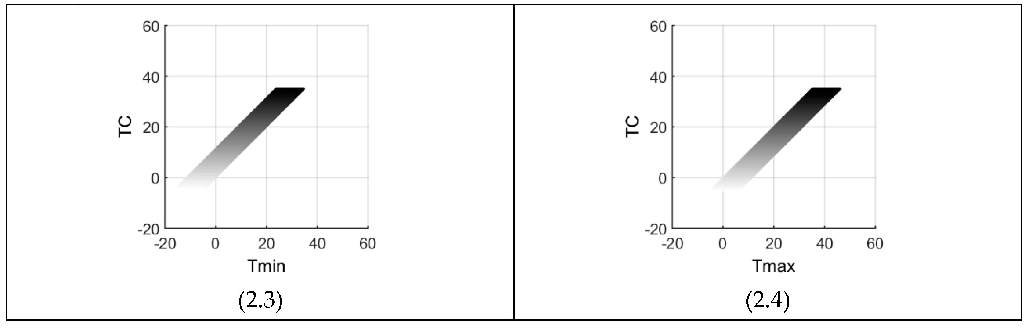
It is needless to mention that Equations (10) and (11) are 3D formulas and utilizing them with the restrictions of Equations (8) and (9) and in conjunction with the thresholds of Table 2, Figure 1 and Figure 2 result each with four sub-figures. There are two conventions used in this work: (A) units of all the variables are centrally given in Table 1, hence throughout the paper, the variables are mentioned without their units; and, (B) four subfigures of any figure are organized in such a way that sub-figure ‘i’ (i: 1 to 4) is in quadrant ‘i’. Both conventions are used throughout this paper about units and numbering of the subfigures. For example, Figure 1(1.3) shows the graph of the pair (Tmin, TR) in the third quadrant of Figure 1. Figure 1(1.1) and Figure 2(2.1) are the 3D graphs with their projections onto the three Cartesian planes as shown in the subsequent sub-figures. All the boundaries of the figures are straight lines with slopes given by Equations (10) and (11), such as 45 degrees (e.g., Figure 1(1.2) and Figure 2(2.3)) and 63.4 degrees (e.g., Figure 1(1.4)) because its tangent is equal to two.
The feasible (Tmin, Tmax) areas are the rectangles shown in Figure 1(1.2) and Figure 2(2.2) with a 45-degree counter clockwise rotation. TR increases in the direction of N-W (North-West) and TC in N-E (North-East), showing orthogonal tendencies on the average. The two figures present and Equations (8) and (9) prove that the highest Tmin has a value equal to TCmax − TRmin/2. The same deductive procedure gives the following limits on Tmin and Tmax:
TCmin − TRmax/2 ≤ Tmin ≤ TCmax − TRmin/2,
TCmin + TRmin/2 ≤ Tmax ≤ TCmax + TRmax/2,
In the cases of Figure 1 and Figure 2, the limits are −16 ≤ Tmin ≤ 34.5 and −4.5 ≤ Tmax ≤ 46, having in mind the thresholds given in Table 2. It is easy to see that not all the combinations of Tmin and Tmax are feasible. For example, the point (10, 33) although within the limits set by Equations (12) and (13) but it is not a feasible point in the region as can be seen from Figure 1(1.2) and Figure 2(2.2) (or Equation (3) and Table 2). An important idea about both of the above inequalities is that knowing the limits on Tmin and Tmax of a region, the four thresholds (TRmin, TRmax, TCmin and TCmax) can be set with confidence by solving four simple equations. Furthermore, Equations (12) and (13) show (i) only positive Tmax values: TRmin > −2 TCmin, such as any positive TCmin value; and, (ii) only positive Tmin and Tmax values: TRmax < 2 TCmin.
Hargreaves and Allen [18] have reported wider monthly limits for the minimum and maximum temperatures used for FPM. However, TC (also used in FPM) and TR have much narrower thresholds as can be seen in FAO-56 and ASCE-EWRI documents. This is, of course, reasonable because of the nature of TC and TR equations. In addition, the existence of temperature thresholds does not mean that they occur on the same day, the same week, nor the same month, which is the period of the wider limits given by Hargreaves and Allen [18]. In summary, any change in TRmin, TRmax, TCmin or TCmax presents an alteration in the rectangular feasible domains of Tmin/Tmax combinations and vice-versa. In general, these insights are useful for data quality control, temperatures in the localities with no data and better understanding of the HS-ETo behaviour as the next subsection demonstrates.
3.2. Performance of HS85
We utilized the methodology explained in the previous section and the 2D graphs of Figure 3, Figure 4 and Figure 5 are some of the results obtained.
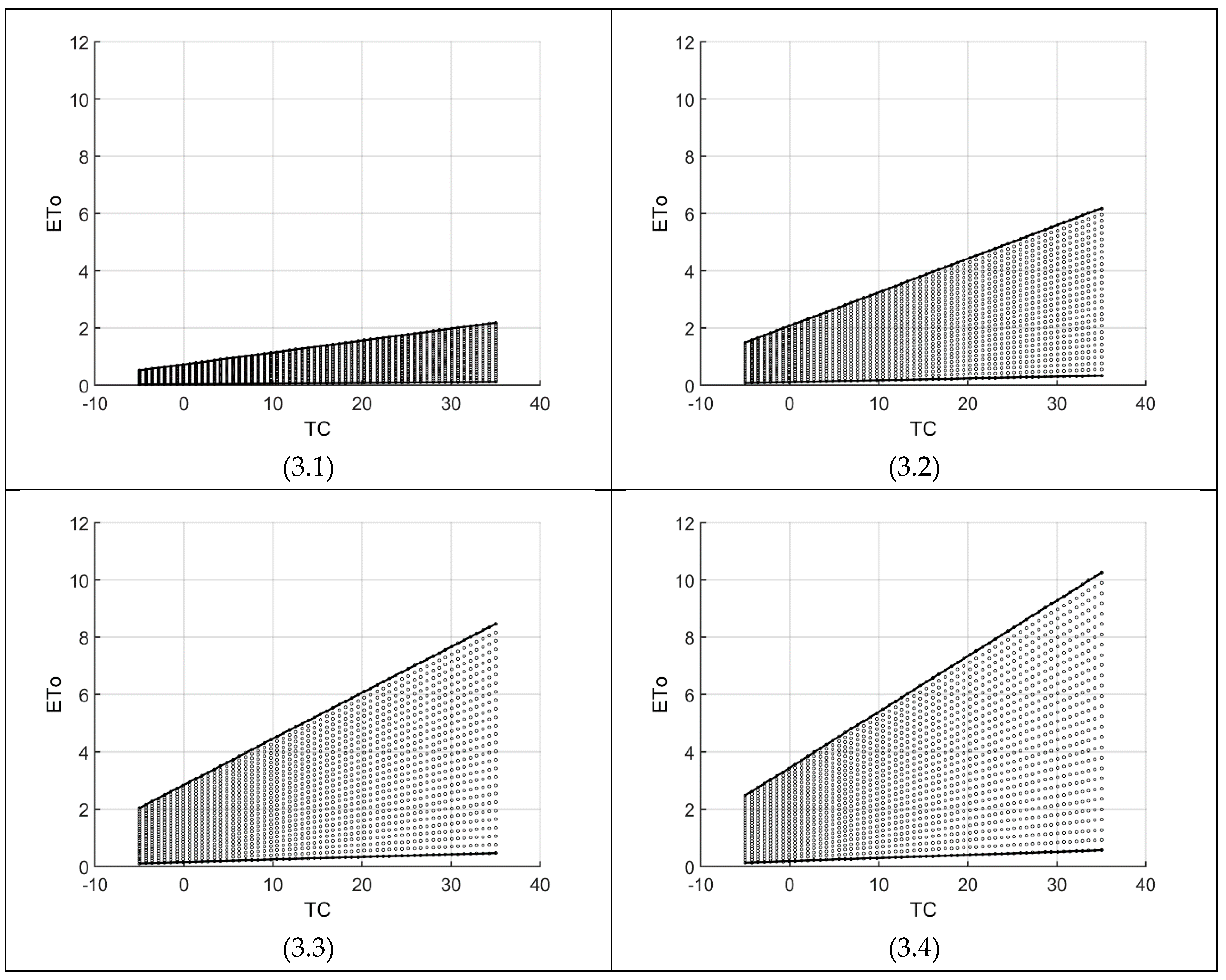
In these figures, four boundaries (left, right, high, low) are visible, presenting the feasible region of HS85. The left and right boundaries (two vertical lines) show the thresholds on the variable representing the horizontal axis. For example, the horizontal axis of Figure 3 is temperature (TC), which varies between −5 and 35 according to Table 2. The high and low boundaries are the limits on the ETo output of the HS85 equation. This means that any ETo value above the high boundary and any value below the low boundary cannot occur according to HS85 and the circumstances set in Table 2. For example, Figure 4(4.3) shows that for RA = 9, HS85-ETo = 4 is not possible, because the equation never calculates values greater than 3.8.
The figures reveal two types of boundaries for the feasible regions: straight line and parabolic that passes through the origin (0, 0). The latter, obviously, occurs if the horizontal axis of a figure displays TR (Figure 5 and Equation (5)). It means that as these values change, ETo varies in a parabolic manner with the horizontal axis as its symmetry. The indirect impact of this nonlinearity is also evident in Figure 4 as will be explained shortly. Another general feature is that if middle values for the three variables are looked upon (somewhat indicative of more occurring values), then HS85-ETo is generally less than five. What follows are some specific results on the three figures, that is, the relationships between the variables of HS85.
Figure 3 presents the changing patterns of ETo along four specific temperature ranges as given in Table 3, that is, TR = {1, 8, 15, 22}. It is the simplest figure showing patterns with a grid of 58 calculation nodes horizontally (TC) and 28 vertically (RA). As the difference between high and low boundaries decreases, for example, at TC = 25 in Figure 3(3.2) relative to TC = 10 of the same figure, the ETo differences between two consecutive nodes also decrease at a constant rate because of linearity. It means that, in HS85, as temperature (TC) decreases, radiation (RA) plays a lesser influence on ETo. Figure 3 also shows that as temperature and temperature range decrease the influence of radiation on ETo decreases down to the point that it becomes negligible. Any increase in temperature (TC) and/or TR would cause an increase in the range of possible ETo values. What follows are two examples:
- (a)
- (b)
- In Figure 3(3.3), 33% increase in TC from 15 to 20 would result in an increase of 15% in the high value of ETo (i.e., the high boundary explained above).
In this setting, the maximum possible ETo is equal to 10.2 and mostly less than six. Consequently, the range of ETo values are easily determined having the maximum and minimum air temperatures. We, of course, remember that in relation to these two temperatures, Figure 1 and Figure 2 are helpful.
Figure 4 shows HS85-ETo patterns along four specific temperatures as given in Table 3, that is, TC = {−5, 8.3, 21.7, 35} with non-regular patterns presented in a grid of 28 × 31 nodes for radiation (RA) and temperature range (TR). As the differential between high and low boundaries decreases, as in Figure 3, the ETo differences between two consecutive nodes also decrease, however, with a decreasing rate due to the nonlinearity introduced by temperature range (TR). Figure 4(4.4) shows this phenomenon better than the others, with a maximum ETo difference of 0.6 (=2.8 − 2.2) for two consecutive nodes. This nonlinearity also indicates that as TR increases, ETo changes decrease (also shown in Figure 5). Any increase in RA and/or TC would cause an increase in the range of possible ETo values. As radiation decreases, the influence of temperature range on ETo decreases down to almost zero (Figure 4(4.1)). For very low radiation, the maximum feasible ETo is 0.6 (Figure 4(4.4)) and for very high radiation, the maximum can go up to 10.2 but mostly below eight (Figure 4(4.3)).
Figure 5 presents nonlinear HS85-ETo patterns along four specific radiations as given in Table 3, that is, RA = {1, 6.7, 12.3, 18} in a grid of 31 × 58 nodes for temperature range (TR) and temperature (TC), respectively. As the difference between high and low boundaries decreases, as in Figure 3, the ETo differentials between two consecutive nodes also decrease with a faster rate due to the nonlinearity introduced by the temperature range. Along one specific TR, the ETo change between two consecutive nodes is constant with a maximum value of 0.14 in Figure 5(5.4). However, the nonlinearity of the high boundary shows that as TR increases, ETo changes decrease (also seen in Figure 4). Any increase in temperature range and/or radiation would cause an increase in the range of ETo possibilities. As TR decreases, the influence of temperature on ETo decreases down to almost zero (Figure 5(5.1)). For the middle values of radiation, that is, Figure 5(5.2,5.3), ETo values are less than about six. For example, for a TR of 15 and RA of nine, ETo is between 1 and 4.2 under any temperature (TC).
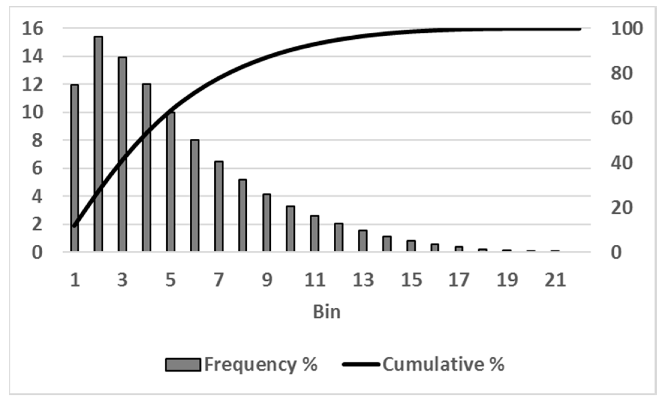
Finally, putting all the valid ETo values into bins or classes, a histogram for HS85 appears in Figure 6. It shows the ETo frequency curve, which reflects the fraction of ETo values in a bin and their cumulative values. As mentioned before, a bin has an ETo value of 0.5.
A total of 50,344 points representing 100% of the total ETo values produce Figure 6 with much skewness to the left. After an initial steep increase, the maximum occurs early in bin two and goes down to zero in bin 22. Ignoring the first bin, that is, ETo values between 0 and 0.5, the frequency and its cumulative curves can be estimated by two second order polynomials with R2 values equal to 99.5% and 98.2%, respectively. The 90% on the Cumulative curve occurs in bin 9, that is, ET values of 4.0 to 4.5.
3.3. Performance of HS00
This subsection presents the results of the modified Hargreaves-Samani (HS00) equation, that is, with a varying KR value as defined by Equation (7). The methodology used is the same as the one employed for the HS85 figures explained previously. This resulted in the three sets of 2D graphs presented in Figure 7, Figure 8 and Figure 9.
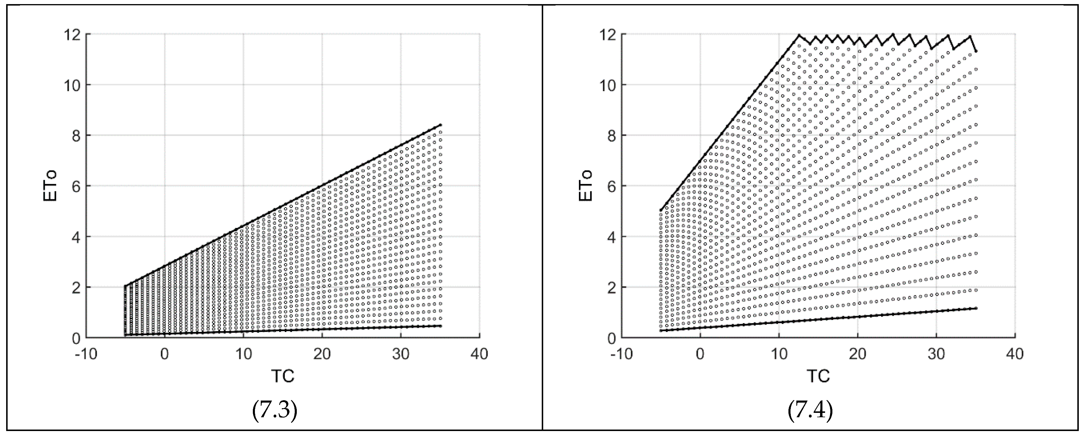
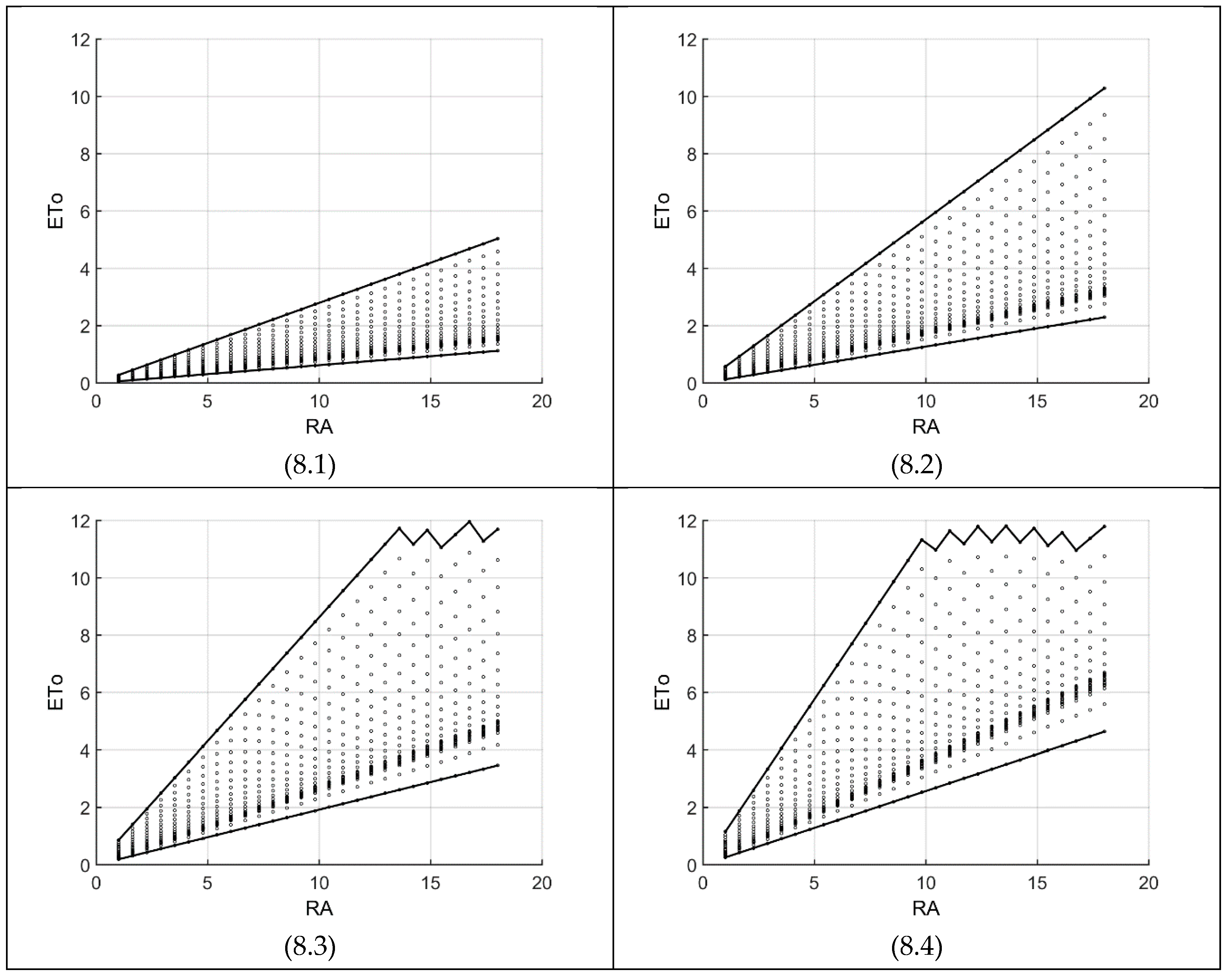
The results in this subsection have some parallels with the ones presented in the previous subsection. On the other hand, some clear changes can also be found. Although the meaning of the four boundaries of the three figures is as explained for HS85 and the left and right boundaries remain unchanged because of the same variable thresholds, the high and low boundaries exhibit much nonlinearity in contrast to the ones for HS85. Most of the high boundaries present bigger values of ETo than the HS85 ones. Using the example given for HS85, Figure 8(8.3) shows that the condition with RA = 9 and ETo = 4 falls into the feasible space (contrary to HS85), because the maximum is HS00-ETo = 7.8 (more than 100% increase relative to HS85).
Figure 7 shows the domain variations along four specific temperature ranges (given in Table 3). As in Figure 3, each graph consists of a maximum grid of 58 × 28 for temperature (TC) and radiation (RA), respectively. As the temperature range (TR) and/or temperature decreases, the impact of radiation (RA) between consecutive nodes reduce substantially. For example, with TC = 10, Figure 7(7.2) gives an ETo difference of about 0.1 between two consecutive nodes but for Figure 7(7.3), it increases by about 35%. On the other hand, increasing RA and TR would lead to a very high range of possible ETo values. For example, one reaches the upper threshold of ETo at a temperature of 12.7 as shown in Figure 7(7.4). The zigzag high boundary of this figure means that the ETo value of the next node for a particular temperature value is more than ETo maximum (=12), hence not included in the feasible space. Consequently, with a higher resolution (more nodes), the zigzag goes toward a horizontal line at ETo = 12. Finally, it is interesting to note that Figure 7(7.2,7.3) are almost identical to Figure 3(3.2,3.3), respectively. The reason is that the KR values calculated by Equation (7) for Figure 7(7.2,7.3), are 0.174 and 0.169, respectively, which are very close to 0.170 used for Figure 3.
Figure 8 is in a maximum grid of 28x31 along radiation (horizontal) and temperature range (vertical), respectively. As the high and low boundaries (corresponding to temperature range thresholds) get closer to each other, the ETo differences between two consecutive nodes decrease toward values less than 0.1 (e.g., Figure 8(8.2)). However, this HS00-ETo difference varies in a nonlinear fashion in two directions (decreasing and then increasing) while HS85 (Figure 4) changes in only one direction. To be clearer, let us look at a few ETo numbers for Figure 8(8.2). For example, for a radiation (RA) of 12, the feasible ETo range varies between 1.5 and 6.8 (seen in Figure 8(8.2)). However, at the start it jumps by 0.3 (between nodes 1 and 2), then rapidly goes down to values less than 0.05 (staying here for 12 nodes) and then increases nonlinearly to 0.6 (between nodes 30 and 31). As already mentioned, Figure 4 presents a different tendency, meaning that delta ETo decreases as the temperature range (TR) increases. The linear low boundary indicating the lowest possible ETo values becomes much steeper meaning that as temperature increases, smaller values of ETo are not feasible according to HS00. For example, for a radiation of 12 in Figure 4(4.3), the minimum possible ETo is 1.1, which is not feasible for HS00 at almost any climatic condition (Figure 8).
Figure 8 is an example of the great influence of Equation (7) on HS85. For example, around the RA ranges of 5 to 15, comparing Figure 8(8.2) with Figure 4(4.2) and Figure 8(8.3) with Figure 4(4.3) reveals more than 100% increase on ETo values (for both low and high boundaries). Under such situations, Tmin must decrease and Tmax increase according to Figure 1. Finally, the zigzag high boundaries of Figure 8(8.3) and Figure 8(8.4) have similar explanations as given for Figure 7(7.4), that is, for each radiation value (e.g., about 13.6 in Figure 8(8.3)), the ETo value of its next node (20 in our case) is more than the maximum (=12), hence is not included in the feasible region. With a higher resolution (more nodes), the zigzag goes toward a horizontal line at ETo = 12.
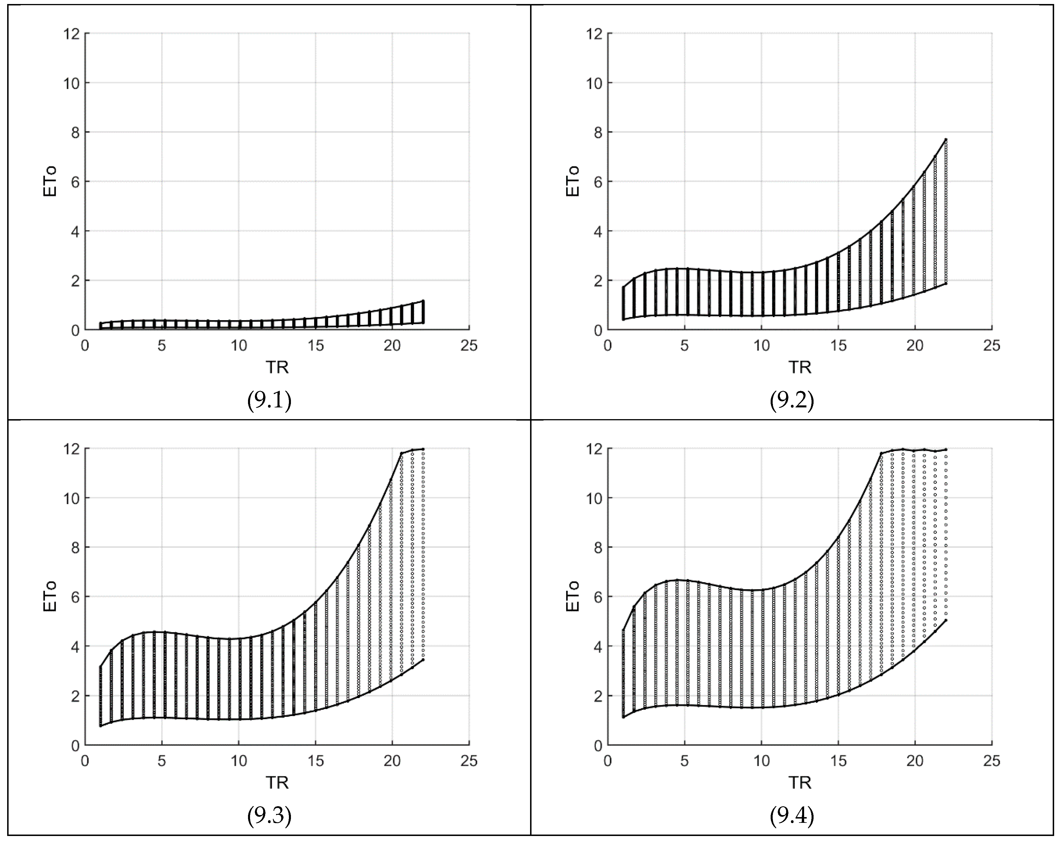
Figure 9 shows the relationship between temperature range (TR) and ETo on four cross-sections along the radiation (RA) domain. The graphs are in a maximum grid size of 31 × 58 and as expected, demonstrate the high nonlinearity of HS00-ETo as a function of TR. As radiation and/or TR decreases, the difference between high and low boundaries also diminishes with a corresponding decrease in the ETo values of two consecutive nodes. Under these conditions, the influence of temperature (TC) continuously diminishes. The maximum delta ETo (i.e., the difference between two consecutive ETo values along a specific TR) is 0.3 for Figure 9(9.4). Mostly, any increase in RA (i.e., among the four graphs) and/or TR (i.e., along the horizontal axis of one of the graphs) would cause an increase in the range of ETo possibilities. Lastly, as explained in the KR Modification subsection above, in the neighbourhood of two temperature ranges (i.e., TR = 8.3 and 15.1), HS00 approaches HS85 with KR = 0.170. Consequently, around these two temperature ranges, Figure 9 gives almost the same ETo values as in Figure 5 because of the concavities in the high boundaries of Figure 9, which are produced by Equation (7).
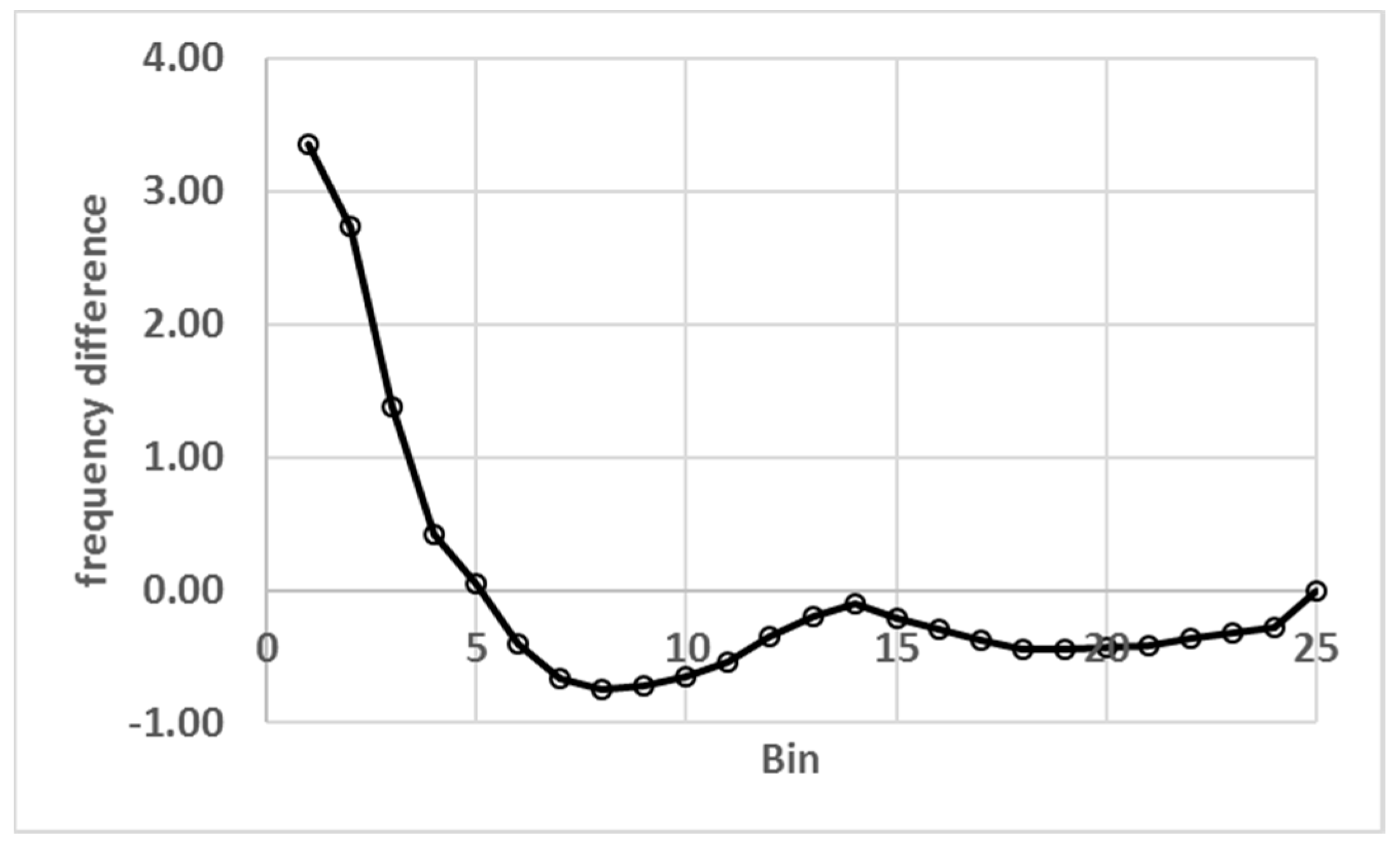
Finally, the HS00 histogram is almost the same as Figure 6 and the maximum of the frequencies still happens in bin 2. Figure 10 shows the differences between the frequencies of HS85 and HS00. There is a steep decrease from 3.4 points of frequency difference to ETo of 2.1 in bin 5 in which the HS85 values are higher than HS00 and then HS00 takes over for the other 20 bins but with smaller changes. In a sense, this was the purpose of the equation presented by Samani [21], however, HS00 creates more nonlinearities than HS85 and consequently it is not clear if it is a better model to estimate ETo.
Existence of the sharp skewness is, of course, consistent with the hyperspace analyses given above. Again, ignoring the first bin, that is, ETo values between 0 and 0.5, the frequency and cumulative curves can be estimated by two second order polynomials with R2 equal to 99.1% and 97.4 %, respectively. The 90% on the cumulative curve occurs in bin 11, that is, ET values of 5.0 to 5.5, indicating up to 25% increase relative to HS85. Figure 10 also shows that HS00 produces more cases where ETo is greater than 2.5 and, consequently, higher values of ETo relative to HS85-ETo.
4. Conclusions
There are two versions of Hargreaves-Samani (HS) for calculating ETo: the 1985 equation with a constant coefficient (HS85) and the same equation but with a varying coefficient introduced in 2000 (HS00). Nobody has performed a study on the nature of these two equations and their inherent behaviour regardless of a specific climatic condition. This introductory paper presents this novel study through 2D graphs that depict the feasible regions and the possible nonlinearity of the models. This is significant for quality control of data and eventually for narrowing down solutions in a particular scenario and making ETo predictions more robust and ultimately automatic (future work).
The mean and range of the temperatures (TC, TR) used in HS effectively define the feasible combinations of Tmin and Tmax and vice-versa. This can guide us in presenting proper temperature values, particularly in areas with no or very sparse real data. For example, the issue of presenting suitable temperature range seems to be the reason for the presentation of HS00 according to its author (refer to the first paragraph of the above subsection “KR Modification”).
Under specific thresholds for the four variables, HS85 is relatively smooth and shows strong nonlinearity among the possible range of ETo values mostly due to the exponent of TR. Within the defined thresholds, passing a straight line through TR0.5 would give R2 = 0.98, making the choice for the exponent of TR questionable. Radiation has a higher influence on possible ETo values as can be seen from Figure 4. HS85-ETo could reach an absolute theoretical maximum of around 10 but mostly less than about six, that is, HS85 can never calculate to the stated threshold of 12.
The effect of KR modification was as intended, that is, increasing ETo hyperspace, particularly on the higher end of the three HS climatic variables. This leads in reaching the ETo maximum threshold of 12 in many situations. On the other hand, the effect of this nonlinear remedy seems unnatural as steep ETo changes occur on both sides of an extended temperature range with little variation in ETo cases (Figure 8 and Figure 9).
It is our expectation that the software HyperET with high resolution can lead us to better understanding of HS and be able to recommend (a work in progress using Artificial Intelligence) as to the near future values of ETo. Such a knowledge combined with performance indicators, such as, Sefficiency, would enable us to advance significantly our scientific approaches and skills to protect our scarce water resources (in nature and in courts).
Author Contributions
Conceptualization, N.H. and R.M.P.; Data curation, N.H.; Formal analysis, N.H. and R.M.P.; Funding acquisition, N.H.; Investigation, N.H. and H.Y.; Methodology, N.H.; Project administration, N.H.; Software, N.H. and R.M.P.; Supervision, N.H.; Validation, N.H. and R.M.P.; Visualization, H.Y.; Writing—original draft, N.H. and H.Y.; Writing—review and editing, H.Y.
Funding
This work was partially financed by (a) the Portuguese Foundation for Science and Technology (FCT) under the contract UID/ECI/04047/2013 for the Centre of Territory, Environment and Construction (CTAC) of the University of Minho, (b) project POCI-01-0145-FEDER-028247 - funded by FEDER funds through COMPETE2020—Programa Operacional Competitividade e Internacionalização (POCI) and by national funds (PIDDAC) through FCT/MCTES.
Acknowledgments
The authors appreciate the cooperation of the Cluster computing facilities of the University of Minho developed under the Project ‘Search-ON2: Revitalization of HPC infrastructure of UMinho’ (NORTE-07-0162-FEDER-000086), co-funded by the North Portugal Regional Operational Programme (ON.2—O Novo Norte), under the National Strategic Reference Framework (NSRF), through the European Regional Development Fund (ERDF).
Conflicts of Interest
The authors declare no conflict of interest. The funders had no role in the design of the study; in the collection, analyses, or interpretation of data; in the writing of the manuscript, or in the decision to publish the results.
References
- NASA and NOAA (2017). NASA, NOAA Data Show 2016 Warmest Year on Record Globally. Release 17–006. Available online: https://www.nasa.gov/press-release/nasa-noaa-data-show-2016-warmest-year-on-record-globally (accessed on 27 February 2017).
- World Economic Forum (2015). Global Risks 2015, 10th ed.; World Economic Forum: Geneva, Switzerland, 2015. [Google Scholar]
- United Nations. Population Division (2015) World Population Prospects: The 2015 Revision. Available online: http://esa.un.org/unpd/wpp/Publications/Files/WPP2015_Volume-I_Comprehensive-Tables.pdf (accessed on 6 June 2016).
- Elferchichi, A.; Giorgio, G.A.; Lamaddalena, N.; Ragosta, M.; Telesca, V. Variability of Temperature and Its Impact on Reference Evapotranspiration: The Test Case of the Apulia Region (Southern Italy). Sustainability 2017, 9, 2337. [Google Scholar] [CrossRef]
- Wang, R.; Bowling, L.C.; Cherkauer, K.A. Estimation of the Effects of Climate Variability on Crop Yield in the Midwest USA. Agric. For. Meteorol. 2016, 216, 141–156. [Google Scholar] [CrossRef]
- Wang, R.; Bowling, L.C.; Cherkauer, K.A.; Cibin, R.; Her, Y.; Chaubey, I. Biophysical and Hydrological Effects of Future Climate Change Including Trends in CO2, in the St. Joseph River Watershed, Eastern Corn Belt. Agric. Water Manag. 2017, 180, 280–296. [Google Scholar] [CrossRef]
- Burt, C.M.; Howes, D.J.; Mutziger, A. Evaporation Estimates for Irrigated Agriculture in California. In Proceedings of the Annual Irrigation Association Meeting, San Antonio, TX, USA, 4–6 November 2001. [Google Scholar]
- Benouniche, M.; Kuper, M.; Hammani, A.; Boesveld, H. Making the User Visible: Analyzing Irrigation Practices and Farmers’ Logic to Explain Actual Drip Irrigation Performance. Irrig. Sci. 2014, 32, 405–420. [Google Scholar] [CrossRef]
- Ahmad, M.; Masih, I.; Giordano, M. Constraints and Opportunities for Water Savings and Increasing Productivity through Resource Conservation Technologies in Pakistan. Agric. Ecosyst. Environ. 2014, 187, 106–115. [Google Scholar] [CrossRef]
- Levidow, L.; Zaccaria, D.; Maia, R.; Vivas, E.; Todorovic, M.; Scardigno, A. Improving Water-Efficient Irrigation: Prospects and Difficulties of Innovative Practices. Agric. Water Manag. 2014, 146, 84–94. [Google Scholar] [CrossRef]
- Ward, F.; Pulido-Velázquez, M. Water Conservation in Irrigation can Increase Water Use. Proc. Natl. Acad. Sci. USA 2008, 105, 18215–18220. [Google Scholar] [CrossRef] [PubMed]
- Haie, N. Sefficiency (Sustainable Efficiency) of Water–Energy–Food Entangled Systems. Int. J. Water Resour. Dev. 2016, 32, 721–737. [Google Scholar] [CrossRef]
- Haie, N.; Keller, A.A. Macro, Meso and Micro-Efficiencies and Terminologies in Water Resources Management: A Look at Urban and Agricultural Differences. Water Int. 2014, 39, 35–48. [Google Scholar] [CrossRef]
- Yen, H.; Hoque, Y.M.; Wang, X.; Harmel, R.D. Applications of Explicitly-Incorporated / Post-Processing Measurement Uncertainty in Watershed Modeling. J. Am. Water Resour. Assoc. (JAWRA) 2016, 52, 523–540. [Google Scholar] [CrossRef]
- Hidalgo, H.G.; Cayan, D.R.; Dettinger, M.D. Sources of Variability of Evapotranspiration in California. American Meteorological Society. J. Hydrometeorol. 2015, 16, 3–19. [Google Scholar]
- Allen, R.G.; Pereira, L.S.; Raes, D.; Smith, M. Crop Evapotranspiration; FAO Irrigation and Drainage Paper 56; FAO: Rome, Italy, 1998. [Google Scholar]
- Hargreaves, G.H.; Samani, Z.A. Reference Crop Evapotranspiration from Temperature. Trans. ASAE 1985, 1, 96–99. [Google Scholar] [CrossRef]
- Hargreaves, G.H.; Allen, R.G. History and Evaluation of the Hargreaves Evapotranspiration Equation. ASCE J. Irrig. Drain. Eng. 2003, 129, 53–63. [Google Scholar] [CrossRef]
- Birhanu, D.; Kim, H.; Jang, C.; Park, S. Does the Complexity of Evapotranspiration and Hydrological Models Enhance Robustness? Sustainability 2018, 10, 2837. [Google Scholar] [CrossRef]
- Estévez, J.; Padilla, F.L.M.; Gavilán, P. Evaluation and Regional Calibration of Solar Radiation Prediction Models in Southern Spain. ASCE J. Irrig. Drain. Eng. 2012, 138, 868–879. [Google Scholar] [CrossRef]
- Samani, Z. Estimating Solar Radiation and Evapotranspiration Using Minimum Climatological Data. ASCE J. Irrig. Drain Eng. 2000, 126, 265–267. [Google Scholar] [CrossRef]
- Laurent, D. 18.330 Introduction to Numerical Analysis. Spring 2012. Massachusetts Institute of Technology: MIT OpenCourseWare. Available online: https://ocw.mit.edu (accessed on 12 October 2018).
- Hargreaves, G.H.; Samani, Z.A. Estimating Potential Evapotranspiration. ASCE J. Irrig. Drain. Div. 1982, 108, 225–230. [Google Scholar]
- Hargreaves, G.H. Moisture Availability and Crop Production. Trans. ASAE 1975, 18, 980–984. [Google Scholar] [CrossRef]
- Samani, Z. Discussion of History and Evaluation of the Hargreaves Evapotranspiration Equation, by Hargreaves, G.H. and Allen, R.G. (2003). ASCE J. Irrig. Drain. Eng. 2004, 129, 53–63. [Google Scholar]
- Hargreaves, G.H. Responding to Tropical Climates. In The 1980–81 Food and Climate Review, the Food and Climate Forum; Aspen Institute for Humanistic Studies: Boulder, CO, USA, 1981; pp. 29–32. [Google Scholar]
- ASCE-EWRI. The ASCE Standardized Reference Evapotranspiration Equation. Appendix B. In Environmental and Water Resources Institute (EWRI) of the American Society of Civil Engineers (ASCE), Standardization of Reference Evapotranspiration Task Committee Final Report; Allen, R.G., Walter, I.A., Elliot, R.L., Howell, T.A., Itenfisu, D., Jensen, M.E., Snyder, R.L., Eds.; ASCE: Reston, VA, USA, 2005; pp. B1–B18. [Google Scholar]
- Allen, R.G. Evaluation of a Temperature Difference Method for Computing Grass Reference Evapotranspiration; Report Submitted to the Water Resources Develop. and Man. Serv., Land and Water Develop. Div.; FAO: Rome, Italy, 1993. [Google Scholar]
- Droogers, P.; Allen, R.G. Estimating Reference Evapotranspiration under Inaccurate Data Conditions. Irrig. Drain. Syst. 2002, 16, 33–45. [Google Scholar] [CrossRef]
- Shahidian, S.; Serralheiro, R.P.; Serrano, J.; Teixeira, J.L. Parametric Calibration of the Hargreaves–Samani Equation for Use at New Locations. Hydrol. Process. 2013, 27, 605–616. [Google Scholar] [CrossRef]
- Tabari, H.; Hosseinzadehtalaei, P.; Willems, P.; Martinez, C. Validation and Calibration of Solar Radiation Equations for Estimating Daily Reference Evapotranspiration at Cool Semi-Arid and Arid Locations. Hydrol. Sci. J. 2016, 61, 610–619. [Google Scholar] [CrossRef]
- Weisstein, E.W. Hyperspace. From MathWorld-A Wolfram Web Resource. Available online: http://mathworld.wolfram.com/Hyperspace.html (accessed on 23 August 2018).
- Loucks, D.P.; Van Beek, E. Water Resources Systems Planning and Management: An Introduction to Methods, Models and Applications; UNESCO: Paris, France, 2005.
Figure 1.
Feasible domains of Tmin and Tmax combinations within the given TR and TC thresholds (darker areas correspond to higher TR values) (units in Table 1).
Figure 1.
Feasible domains of Tmin and Tmax combinations within the given TR and TC thresholds (darker areas correspond to higher TR values) (units in Table 1).

Figure 2.
Feasible domains of Tmin and Tmax combinations within the given TR and TC thresholds (darker areas correspond to higher TC values) (units in Table 1).
Figure 2.
Feasible domains of Tmin and Tmax combinations within the given TR and TC thresholds (darker areas correspond to higher TC values) (units in Table 1).


Figure 3.
ETo as a function of temperature (TC) in the Hargreaves-Samani 1985 equation. The four specific cross-sections (sub-figures) are along the temperature range (TR) with radiation (RA) varying within its thresholds (units in Table 1).
Figure 3.
ETo as a function of temperature (TC) in the Hargreaves-Samani 1985 equation. The four specific cross-sections (sub-figures) are along the temperature range (TR) with radiation (RA) varying within its thresholds (units in Table 1).

Figure 4.
ETo as a function of radiation (RA) in the Hargreaves-Samani 1985 equation. The four specific cross-sections (sub-figures) are along the temperature (TC) with temperature range (TR) varying within its thresholds (units in Table 1).
Figure 4.
ETo as a function of radiation (RA) in the Hargreaves-Samani 1985 equation. The four specific cross-sections (sub-figures) are along the temperature (TC) with temperature range (TR) varying within its thresholds (units in Table 1).


Figure 5.
ETo as a function of temperature range (TR) in the Hargreaves-Samani 1985 equation. The four specific cross-sections (sub-figures) are along the radiation (RA) with temperature (TC) varying within its thresholds (units in Table 1).
Figure 5.
ETo as a function of temperature range (TR) in the Hargreaves-Samani 1985 equation. The four specific cross-sections (sub-figures) are along the radiation (RA) with temperature (TC) varying within its thresholds (units in Table 1).

Figure 6.
ETo histogram and its cumulative frequencies for the Hargreaves-Samani 1985 hyperspace with a bin value of 0.5 mm/day.
Figure 6.
ETo histogram and its cumulative frequencies for the Hargreaves-Samani 1985 hyperspace with a bin value of 0.5 mm/day.

Figure 7.
ETo as a function of temperature (TC) in the modified Hargreaves-Samani equation. The four specific cross-sections (sub-figures) are along the temperature range (TR) with radiation (RA) varying within its thresholds (units in Table 1).
Figure 7.
ETo as a function of temperature (TC) in the modified Hargreaves-Samani equation. The four specific cross-sections (sub-figures) are along the temperature range (TR) with radiation (RA) varying within its thresholds (units in Table 1).


Figure 8.
ETo as a function of radiation (RA) in the modified Hargreaves-Samani equation. The four specific cross-sections (sub-figures) are along the temperature (TC) with temperature range (TR) varying within its thresholds (units in Table 1).
Figure 8.
ETo as a function of radiation (RA) in the modified Hargreaves-Samani equation. The four specific cross-sections (sub-figures) are along the temperature (TC) with temperature range (TR) varying within its thresholds (units in Table 1).

Figure 9.
ETo as a function of temperature range (TR) in the modified Hargreaves-Samani equation. The four specific cross-sections (sub-figures) are along the radiation (RA) with temperature (TC) varying within its thresholds (units in Table 1).
Figure 9.
ETo as a function of temperature range (TR) in the modified Hargreaves-Samani equation. The four specific cross-sections (sub-figures) are along the radiation (RA) with temperature (TC) varying within its thresholds (units in Table 1).

Figure 10.
Percentage point frequency differences between the histograms of HS85 (Figure 6) and HS00.
Figure 10.
Percentage point frequency differences between the histograms of HS85 (Figure 6) and HS00.


Table 1.
Symbols, descriptions and units of the variables used in the Hargreaves-Samani equation.
| Symbol | Description | Units |
|---|---|---|
| ETo | Reference crop evapotranspiration | mm/day |
| KH | Coefficient in Hargreaves-Samani equation | -- |
| KR | Empirical coefficient for the radiation formula | -- |
| RA | Extra-Terrestrial radiation | mm/day |
| RS | Global solar radiation at the surface | mm/day |
| TC | Mean air temperature | °C |
| Tmax | Maximum air temperature | °C |
| Tmin | Minimum air temperature | °C |
| TR | Temperature range | °C |
Table 2.
Thresholds of the I/O variables of the Hargreaves-Samani equation (units in Table 1).
Table 2.
Thresholds of the I/O variables of the Hargreaves-Samani equation (units in Table 1).
| Variable | Minimum | Maximum |
|---|---|---|
| ETo | 0 | 12 |
| RA | 1 | 18 |
| TC | −5 | 35 |
| TR | 1 | 22 |
Table 3.
Information about nodes and cross sections (cuts = 4) of each variable (units in Table 1).
Table 3.
Information about nodes and cross sections (cuts = 4) of each variable (units in Table 1).
| Variable | Difference between Consecutive Nodes | Total Nodes | Difference between Consecutive Cuts | Nodes of the Cuts |
|---|---|---|---|---|
| RA | 0.63 | 28 | 5.7 | 1, 10, 19, 28 |
| TC | 0.70 | 58 | 13.3 | 1, 20, 39, 58 |
| TR | 0.70 | 31 | 7.0 | 1, 11, 21, 31 |
© 2018 by the authors. Licensee MDPI, Basel, Switzerland. This article is an open access article distributed under the terms and conditions of the Creative Commons Attribution (CC BY) license (http://creativecommons.org/licenses/by/4.0/).
Share and Cite
MDPI and ACS Style
Haie, N.; Pereira, R.M.; Yen, H. An Introduction to the Hyperspace of Hargreaves-Samani Reference Evapotranspiration. Sustainability 2018, 10, 4277. https://doi.org/10.3390/su10114277
AMA Style
Haie N, Pereira RM, Yen H. An Introduction to the Hyperspace of Hargreaves-Samani Reference Evapotranspiration. Sustainability. 2018; 10(11):4277. https://doi.org/10.3390/su10114277
Chicago/Turabian StyleHaie, Naim, Rui M. Pereira, and Haw Yen. 2018. "An Introduction to the Hyperspace of Hargreaves-Samani Reference Evapotranspiration" Sustainability 10, no. 11: 4277. https://doi.org/10.3390/su10114277
Note that from the first issue of 2016, this journal uses article numbers instead of page numbers. See further details here.