The Secret to Getting Ahead Is Getting Started: Early Impacts of a Rural Development Project

Abstract

Interventions in rural development projects vary in their likely time to impact. Some offer rapid payoffs after minimal learning and investment, while others offer larger payoffs but entail delays and may require learning or significant investment of labor and capital. Short-term impacts included reductions in stored grain losses due to improved silos and increase in household savings due to increased participation in savings groups. The least poor are most likely to invest labor and capital in slow-to-accrue payoffs like soil erosion abatement from building conservation structures. Our results suggest that targeting project interventions by asset level can enhance impacts.

1. Introduction

Despite efforts to reduce poverty worldwide, rural areas still lag behind. Of the 1.4 billion people living with less than $1.25 a day, around 70% lived in rural areas, and a total of 80% of the rural population has agriculture as its livelihood [1]. Adoption of improved agricultural technologies has the potential to reduce poverty by increasing production for home consumption, by raising revenues from sales, or by reducing production costs [2,3]. Adoption of high yield varieties (HYV) and complementary modern inputs such as fertilizers have been proven to increase income and reduce poverty [4,5,6,7]. Sustainable agricultural technologies, such as conservation agriculture practices and the construction of soil conservation structures, have the potential to reduce poverty by increasing productivity and improving food security by reducing land degradation [8]. These technologies are likely to increase yields, and improve soil and water quality when successfully adopted [9]. Improved storage technologies such as hermetic metallic silos can reduce stored grain loses and trigger longer-term impacts on nutrition and income [10].

In spite of the potential benefits, adoption of sustainable agricultural technologies is still low among smallholder farmers in the developing world [11,12]. Recently, some conservation technologies have been promoted under the label of climate smart agriculture to promote sustainable agricultural intensification and to contribute to food security [13,14]. Lack of credit, input and output market failure, land and labor constraints, and lags between adoption and perceived benefits [15,16] are among the reasons for low adoption rates. Agricultural development projects promote interventions to overcome these barriers. After a half-century of rural development projects with mixed results, donors have come to insist on rigorous impact assessment. However, evidence on the effectiveness of sustainable agricultural technology interventions is still relatively scarce in the literature.

Recent evaluations have focused on the impacts on productivity and cash income of Green Revolution-type technologies, such as improved seed varieties and fertilizer [17,18,19,20,21,22,23]. Few studies have evaluated early impacts of development strategies in the take up of agricultural technologies at early stages of project implementation [24,25]. Largely ignored has been the discussion of timing of project effects [26], especially early effects on adoption of changed practices that yield rapid benefits or that put framers on a promising trajectory for large, subsequent welfare impacts.

In this article, we explore the impacts of a project that promoted a package of interventions on adoption, intensity of adoption, and early impacts of adoption. We discuss the timing of different interventions to impacts, how different subsets of households benefitted from project interventions, test for robustness of our impact estimates using different impact evaluation methods, and discuss pathways from early adoption for sustainable incomes and resource conservation. The focal project for this study promoted conservation agriculture practices and soil conservation investments, improved storage technologies, together with an informal saving and lending scheme. Savings have been promoted together with agricultural technologies to stabilize consumption over time and alleviate constraints to adoption [27]. We evaluated the project after [28] months of project implementation. The timing of the evaluation survey enables measurement of new practices adopted and of short-term impacts, such as reduction in stored grain losses.

Treatment is defined as the exposure to the package of interventions. Exposure means having knowledge about the interventions, their characteristics, and their benefits. When the elements of the package are divisible, farmers will tend to adopt elements of the package instead of the package as a whole as a strategy to reduce costs and risks of adoption [28,29,30]. Partial adoption of the package can also bring benefits to project participants [31], for this reason we evaluate the adoption of package elements.

Turnkey technologies like improved grain storage silos require little special knowledge to adopt or to use, and they can be expected to reduce storage losses rapidly, contributing to net household income. When projects promote interventions that demand special learning or cumulative effort, such as conservation agriculture technologies, impacts tend to accrue gradually [32,33]. The greatest impacts of soil conservation technologies occur under extreme rainfall conditions [34], which by definition are infrequent. When the effects are manifested, they often entail a loss of income rather than a gain. All of these factors imply that the impact of adoption of soil conservation technologies tend to occur after long delays. The upshot is that some project interventions may be expected to show early impacts (say, within two years), whereas others could take decades.

A concern for impact assessment was that project beneficiaries were not randomly assigned to treatment. First, the project was targeted at the poor. Second, eligible households could self-select to participate in project interventions. To control for these two sources of selection bias we estimate impacts using difference-in-difference propensity score matching (DID-PSM), and check for robustness of our results using difference-in-difference matching in covariates, and inverse propensity score weighting (IPSW), and difference-in-difference (DID) estimation.

Our results suggest that the project increased adoption of improved agricultural practices, promoted soil conservation investments, reduced stored grain losses, and increased household savings. The results also show that relative asset levels shaped which households adopted which technologies and practices. Households with low levels of assets increased savings, while households with high and medium levels of assets invested more in soil conservation structures. Targeting of interventions according to asset level, and phasing interventions for the poorest, arises as a recommendation to improve the design of interventions that promote a package of interventions with different levels of investment and timing to achieve project impacts.

This article continues with a description of the project to be evaluated, the process for targeting beneficiaries, a conceptual framework for the analysis of project impacts, the description of the survey data, the methods for evaluating project impacts, and the presentation of results and conclusions.

2. The A4N Project

2.1. The Project

Catholic Relief Services and its partners in Central America implemented the Agriculture for Basic Needs (A4N) project during 2009–2012. The project promoted conservation agriculture practices and construction of agricultural conservation structures, training in post-harvest management, storage practices, and use of metallic silos for storage of grains. The project provided metallic silos to farmers and training on storage practices, and taught farmers how to build conservation structures with locally available materials and at low cost. The project promoted the formation of producer groups, trained farmers in farmer field schools, and provided farm-level technical assistance. The project addressed financial market failure by the promotion of saving and lending groups, trained farmers in basic financial skills, and provided saving groups with materials such as paper and pencils to keep records.

All participating households were encouraged to form groups to access A4N training on specific practices. Beneficiary households were expected to participate in multiple group activities. For instance, about 70% of beneficiaries in our sample participated in at least three different training topics, with households participating in different combinations of training activities from conservation agriculture, to savings and storage management. There were also different household members affiliated with different groups formed by the project.

2.2. From Intervention to Project Impacts

There were three main mechanisms for A4N to achieve project impacts. First, adoption of conservation agriculture practices and soil conservation investments is expected to stabilize and increase yields. Reduced tillage practices can reduce labor needs during planting and land preparation in the short term, reducing labor costs, so long as weed control is not labor intensive and costly. Soil conservation investments are expected to prevent degradation and aid in soil recovery [34], stabilizing soil and yields in the long term. Soil conservation also has the potential to increase resistance to extreme weather events [35].

Second, metallic silos for grain storage are expected to reduce post-harvest losses. These hermetically sealed structures reduce grain exposure to pests and humidity [10,36]. Adoption of silos is likely to reduce the need to buy grain in periods of household food deficit (which often correspond with high prices), improving food security. Improved silos can increase revenues during good years by increasing marketable surplus and by enabling delay of grain sales beyond the immediate post-harvest period when prices are typically at their nadir.

Third, savings allow farmers to smooth consumption over the year and reduce the risk of asset liquidation during periods of food scarcity—or when other shocks occur [37].

2.3. Selection of Project Beneficiaries

Two different processes led to nonrandom participation in specific A4N interventions. First, the project was targeted at the poor, so participants in the A4N project differed from non-participants in observable characteristics. Second, the self-selection of individuals into A4N means that unobservable traits may also have affected project participation.

The A4N project targeted villages considered poor, in terms of limited access to basic services such as water and sanitation, predominance of small land holdings, and reliance on production of staple grains (maize and beans). Within these villages, poor farmers were eligible to participate in the project. The project established a set of criteria as a guide to determine eligibility: cultivated land area less than 1.73 acres; cultivated land on steep slopes; lack of access to any of the following public services: Piped water, sanitation, and electricity; materials for house walls not brick or concrete; roof not zinc or brick; floor not concrete, ceramic, or tile; household experiences hunger during some period of the year; household head is female; household includes children younger than five years old. These eligibility criteria, together with farm and village characteristics, are used later in the paper to estimate the probability of participation in the A4N project (propensity score) for PSM-DID and IPSW estimation, and to conduct matching in covariates.

3. Conceptual Framework

Farmers are assumed to make technology choices that maximize their expected utility over time. Adoption of new technologies implies costs of learning and other costs. These costs could take the form of time to acquire information about the use and benefits of a new technology and/or to obtain labor and purchased inputs [29,38]. Learning and experimentation with new technologies allow adaptation and decisions on whether the technologies are suitable for individual farm conditions [33,39].

For smallholder farmers, lack of information about new technologies and constraints on financial liquidity, labor, or learning time can impede adoption of practices requiring investments [40,41]. The A4N project not only made technologies known to farmers through training and information dissemination, but also promoted local financial institutions, such as lending and saving groups, to improve project participants’ credit capacity. The fact that the project offered a package with several component technologies complementary each other would also make adoption even more likely [42]. Hence, it is expected that the project will have an unambiguously positive effect on a farmer’s likelihood to adopt all the technologies promoted by the project, regardless of whether they have immediate payoff or delayed payoff.

Unlike its effect on farmer’s adoption decision, the short-term welfare impacts of the project (28 months after project implementation) depend on the type of the technology adopted, the site-specific agro-ecological condition, and socio-economic condition of the adopter [43]. Specifically, conservation agriculture technologies require high up-front investments, whereas some of the benefits accrue gradually, whereas others may not be realized until an extremely erosive rain event. Construction of soil conservation structures requires land and labor, as well as working capital to cover the costs of materials and maintenance [44]. Reduced tillage tends to reduce labor requirements for tillage, but it demands increased cash outlays for herbicides and often some added labor time for hand weeding. Because of the high investments and the delays of conservation agriculture technologies to provide returns to investments, larger farmers, with more farm resources and longer time horizons, have been found to adopt these technologies more readily [31]. Equally important, as noted above, even after adoption, is that the time lag to measurable welfare impacts tends to be long.

Conservation agriculture is a complex technology that often involves change in the farming system. It is more knowledge intensive than input intensive, and successful implementation depends on what the farmer does and how the farmer does it, rather than which external inputs he applies. Conservation practices tend to require experimentation and adaptation to farmers’ particular needs and conditions [45]. Benefits in the form of averted yield decline and reduced yield variability from soil conservation investments are realized only gradually and unevenly, with the greatest benefits occurring under rare, extreme rainfall conditions [46]. In technology adoption models with emphasis on learning and experimentation, farmers tend to adopt the new technology, as long as the expected future gains are higher than the old one [32,33,39].

Unlike conservation technologies that take time to adopt and to show benefits, turnkey technologies such as metallic silos are easier to learn and adapt. Adoption of hermetically sealed silos is likely to sharply reduce losses compared to open granaries, sacks, and barrels [36]. Likewise, once the silos have been provided by the project and farmers trained in their use, benefits from adoption are perceived after one cropping season 10. Once the saving and lending groups are formed, members start receiving loans within three months of membership, and in less than eight months group members can claim their savings plus interest.

In order to measure early impacts of the A4N project, three hypotheses are tested empirically. Each is presented in terms of the hypothesis that we expect to be true (rather than in null form):

Hypothesis 1 (H1).

The A4N project increased adoption of the practices that it promoted.

Hypothesis 2 (H2).

Project benefits depend on the time horizon of the intervention, such that:

Hypothesis 2a (H2a).

Interventions that require little investment or learning to show results (e.g., savings groups and storage losses) will show impacts after just 28 months.

Hypothesis 2b (H2b).

Interventions that require (a) substantial investment of labor and/or capital or (b) learning or (c) infrequent extreme conditions to show results (e.g., conservation structures) will result in behavioral changes (in the form of adoption) just after 28 months.

Hypothesis 3 (H3).

Households will benefit differently from the project interventions according to asset levels.

4. Methodology

To control for potential selection bias in exposure to project interventions, we estimate impacts using quasi-experimental econometric methods. In an ideal situation, project beneficiaries would have been randomly assigned. The project design did not allow for this. The project-based access to participation at both the village and household levels on a set of eligibility criteria that emphasized poverty status. In order to control for non-random assignment to the project treatment, we use difference-in-difference propensity score matching (DID-PSM) and compare our estimates with difference-in-difference matching in covariates, difference-in-difference inverse propensity score weighting (IPSW), and difference-in-difference (DID) estimation.

4.1. Evaluation of Project Impacts

4.1.1. Propensity Score Methods

Propensity score matching (PSM) consists of choosing the comparison group according to the probability of being selected for a treatment, given a set of observable pre-treatment characteristics and outcome values that do not change with program intervention but which affect program placement. PSM assumes that program outcomes are independent of the status of program participation, conditional on observable characteristics (unconfoundedness), and common support or overlap between the probability distribution of program participants and non-participants [47,48,49]. To estimate the propensity score (PS), we include a rich set of variables that determine both participation in the project and farm and village pretreatment characteristics to reduce bias in estimates [50].

By using the PSM-DID estimator, we control for observable sources of bias by building our comparison group using PSM as well as time invariant characteristics, by taking the difference of outcomes before and after treatment (DID). The PSM-DID estimator, defined by Smith and Todd [51], is as follows:

$${\widehat{\tau }}_{ATT, PSM-DID}=\frac{1}{N_1}{\displaystyle \sum }_{jϵI_1{\displaystyle \cap }{S}_p}\{\left(y_{1it}-y_{1it-1}\right)-{\displaystyle \sum }_{jϵI_0{\displaystyle \cap }{S}_p}\phi \left(i,j\right)\left(y_{0it}-y_{0it-1}\right)\}$$

(1)

As an additional robustness check, we conduct inverse propensity score weighted regression (PSW) [52,53,54], in the panel data context we take the difference between outcomes before and after treatment:

$${\widehat{\tau }}_{ATT, PSM}=\frac{1}{N}{{\displaystyle \sum }}_{i=1}^N\frac{\left(A4N-\widehat{\mathrm{Pr}}\left(x_i\right)\right)\left(y_{it}-y_{it-1}\right)}{\widehat{\rho }\left(1-\widehat{\mathrm{Pr}}\left(x_i\right)\right)}$$

(2)

For Equations (1) and (2), the subscripts 1 and 0 refer to treated and untreated, respectively, S_p refers to the common support, t refers to the time period, N to the total number of observations, ϕ(.) is a weight that depends on the matching method used, Pr(x_i) is the propensity score, and ρ refers to the proportion of treated observations in the sample (N₁/N). For the weighted regression we also include the difference of time variant covariates in the PSW regression.

We also conduct matching in covariates [55,56]. This estimator consists of matching all units, treated and comparison, using the distance between the values of the covariates for each observation (using the malahanobis distance in our case). We match observations on the covariates included in the propensity score. The matching can be conducted with one or more observations (one in our case). Since matching multiple covariates can lead to substantial bias, it is combined with bias adjustment to remove most of the bias. This approach uses linear regression to remove the bias associated with differences in the matched values of the covariates [56,57].

4.1.2. Regression Methods

The main assumption of DID is that the unobserved differences between participants and non-participants are invariant in time. Examples would be particular individual characteristics, like motivation and cognitive ability. By taking the first difference, we removed time invariant unobservable characteristics. Then, obtaining the difference between periods t and t − 1, the unobservable characteristics, assumed invariant in time are eliminated, controlling for this source of bias in the program impact estimation [54]:

$$∆y_{it}={\alpha }_0+\tau A4N_i+\beta ∆x_{it}+∆u_{it}$$

(3)

where ∆y_it = y_it − y_it−1, Δx_it = x_it − x_it−1, and Δu_it = u_it − u_it−1. We obtain the program impact by the regression of the change in the outcome variable y on the project participation variable A4N, and the change in a set of time varying covariates x. The parameter of interest to estimate is τ, the difference in difference estimator. Standard errors are adjusted for clustering effect at the village level.

The difference in difference estimator assumes parallel trends for both treatment and comparison in the absence of the treatment [58]. Therefore, correcting for differences between the two groups requires controlling for covariates related to household characteristics [58]. To take care of possible differences of covariates between treatment and comparison, the time varying covariates likely to influence adoption include household size, average years of education of household members, total area of cultivated land, and proportion of land allocated to annual crops.

4.1.3. Program Impacts by Asset Level

Project impacts can vary among subsets of individuals or households. In particular, differential impacts by asset level have been noted elsewhere [59,60]. We estimate project impact on outcome y for each of group of households in asset level g. The heterogeneity of program effects can also be estimated as follows:

$$∆y_{it}={\alpha }_0+\beta ∆x_{it}+\tau A4N_i+\delta D_{ig}+\rho \left(A4N_i\times D_{ig}\right)+∆u_{it}$$

(4)

where D_g a set of dummy variables to identify each of asset level group (excluding the reference group). Empirically, asset levels are proxied by cropland owned. The vector of parameters of interest are τ and ρ.

5. Survey Data Used for Evaluation of Impacts

The dataset comes from a two-stage survey of treatment and non-treatment villages. We randomly sampled villages from the list of beneficiary villages, and paired them with similar non-participant villages using Nicaraguan population and agricultural census data. The sampled treatment villages were selected according to the population weights of each of the municipalities where the project intervened. Comparison villages were identified according to national census data on poverty levels, as measured by the index of unmet basic needs, the importance of staple crops, small-sized landholdings [61], and location in the same agrarian zones [62]. From each village we randomly selected 10 treated households in the participant villages and 10 to 15 households in the non-participant villages, depending on village size. For the A4N villages, CRS provided lists of treated households. Eligible beneficiaries in participant villages had access to the project, benefiting from household and/or village level interventions. In non-participant villages, sample lists were developed in consultation with village leaders, who were requested to identify households that would meet the eligibility criteria of the A4N program. No eligible but untreated households were identified in the A4N participant villages, so no such households could be included in the sample.

A baseline survey was conducted for the agricultural year 2008–2009, preceding project implementation. A follow up survey did the same for the agricultural year 2010–2011, the second year after project implementation and eight months before project end. The survey information covered livelihoods, farm activities, the technologies and practices implemented by farmers, their postharvest storage practices, their participation on saving groups, and the revenues and costs of farm activities. The survey was conducted in the departments of Estelí, Jinotega, and Matagalpa, located in north-central Nicaragua. The final balanced panel included 576 households in each round of data collection. The attrition rate between the two rounds of the survey was 7%, and we found no significant systematic differences in the mean values of key household, household head, farm, and village characteristics between the panel households and attrited households (available but not reported). A parallel village survey documented village-level characteristics. The final household sample includes 282 households in 30 treated (A4N participant) villages and 294 households in 30 comparison (non-participant) villages in the baseline and follow up.

6. Research Results: A4N Project Impacts

We estimated the probability of participation in A4N using a set of pretreatment characteristics that include household and housing characteristics, farm characteristics, asset endowments, and village characteristics. We followed standard procedures from Imbens [56], Imbens and Wooldridge [48], and Wooldridge [54]. Most of the variables included correspond to variables related to the project eligibility criteria. We estimated the PS using logit. We trim a total of 11 observations with PS higher than 0.90 and lower than 0.10 and re-estimated the PS (Appendix A

Table A1. Probability of program participation using logit.

Dependent Variable: A4N = 1
Explanatory Variables	Coef.	Std. Err.
Cultivated land Mz	0.03	(0.03)
Steep slope = 1	0.20	(0.20)
Inadequate services = 1	−0.54 **	(0.22)
Inadequate housing = 1	0.09	(0.29)
Electricity = 1	0.01	(0.21)
Hunger = 1	0.37 *	(0.20)
head female = 1	1.19 ***	(0.30)
#children <5	0.06	(0.14)
head age	0.00	(0.01)
head education	−0.01	(0.04)
household size	−0.05	(0.06)
people per room	−0.03	(0.06)
Infraestructure C$/1000	−0.09	(0.06)
Livestock C$/1000	−0.02 **	(0.01)
Equipment C$/1000	0.00	(0.02)
Population 2009	0.00	(0.00)
Dist. Market Km/10	−0.05 ***	(0.01)
Dist. Paved road Km/10	0.02	(0.01)
Health facility = 1	−0.82 ***	(0.26)
% basic grains 2003	−0.19	(0.63)
% lanholdings <10 Mz 2003	2.40 ***	(0.49)
Constant	−0.19	(0.84)
n	564
Log likelihood	−350.68

Levels of significance *** 1%, ** 5%, * 10%.

).

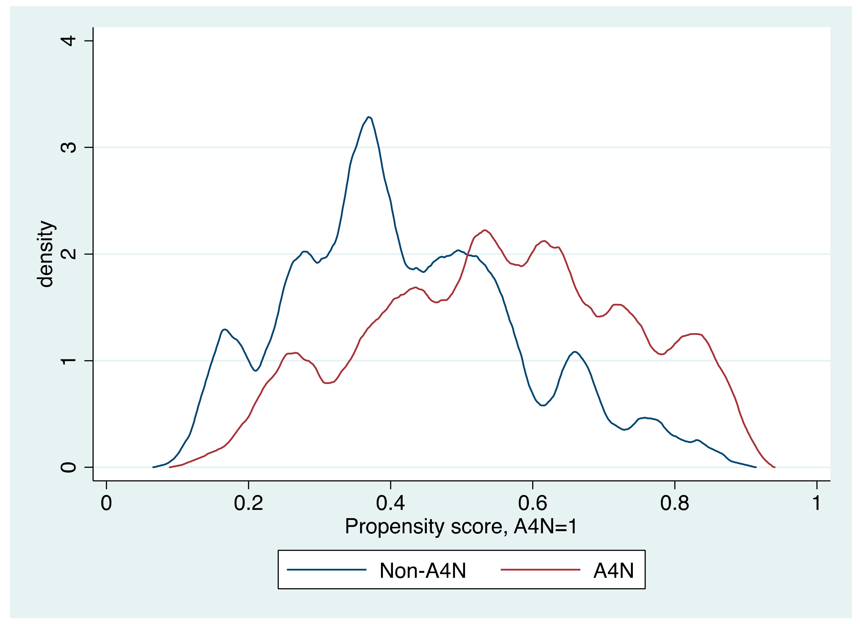
Using this estimation, we check for overlap between the treatment and comparison, we plotted the marginal distributions for the treated and the comparison group (Figure 1). The comparison group distribution contains more observations with propensity scores below 0.6, and a disproportionate number of observations with propensity scores below 0.4. In spite of this, overlap does not seem to be a problem, and we have comparison observations to match treatment ones (Figure 1) [63]. In

Table 1. Balancing tests of pretreatment covariates used for estimation of the propensity score. Nicaragua, 2009.

Variable	Before Matching				After Matching
	Mean				Mean
	Treated	Comparison	t-test	%bias	Treated	Comparison	t-test	%bias
Cultivated land Mz	3.29	3.5	0.56	−2.68	3.31	3.38	0.83	−1.6
Steep slope = 1	0.32	0.32	0.81	−25.87	0.32	0.36	0.32	−9.7
Inadequate services = 1	0.66	0.79	0.00	21.39	0.68	0.65	0.53	3.6
Inadequate housing = 1	0.88	0.85	0.36	60.1	0.88	0.88	1.00	4.4
Electricity = 1	0.61	0.63	0.55	15.32	0.60	0.57	0.44	4.9
Hunger = 1	0.39	0.32	0.13	−17.89	0.38	0.45	0.08	−4.2
Head female = 1	0.2	0.07	0.00	−73.06	0.18	0.18	0.82	−12.8
Children <5 years old	0.51	0.51	0.94	−24.23	0.51	0.50	0.82	14.1
Head age	49	48	0.25	68	49.17	49.77	0.63	−1.2
Head education	2.83	3.04	0.37	3.13	2.84	2.51	0.12	1.7
Household size	5.2	5.36	0.45	49.55	5.21	5.23	0.94	9.3
People per room	3.82	3.86	0.76	40.94	3.86	3.85	0.96	−0.6
Infrastructure C$/1000	0.53	0.80	0.10	−21.5	0.53	0.60	0.63	3.3
Livestock C$/1000	6.71	9.07	0.05	−17.33	6.80	5.68	0.18	5.7
Equipment C$/1000	1.76	2.08	0.55	−49.91	1.79	1.59	0.55	−6.2
Population 2009	637	640	0.88	16.68	642.77	645.33	0.96	−5.9
Dist. Market Km/10	14.09	16.29	0.00	38.19	14.24	14.34	0.89	−1.5
Dist. Paved road Km/10	9.53	8.95	0.41	−0.99	9.61	10.01	0.63	10
Health facility = 1	0.21	0.28	0.07	−37.29	0.21	0.22	0.92	0.7
% Basic grains 2003	0.86	0.88	0.26	71.93	0.86	0.88	0.14	−4.9
% Landholdings <10 Mz 2003	0.59	0.52	0.00	64.34	0.58	0.55	0.07	18

1 Mz = 1.73 Acres U$1 = C$22.42 p-values correspond to a t-test for equal means. $\% bias=\frac{\overline{x_{1j}}-\overline{x_{2j}}}{\sqrt{s_{1j}^2-s_{2j}^2}}\times 100$. Source: A4N Baseline Household Survey 2010, Baseline Village Survey 2010, Nicaragua Agricultural Census 2003.

we present the balancing test to show how matching improved overlap between the probability distributions of the treatment and the comparison group. As shown by the t-test for equal means for the pretreatment characteristics of these two groups, we find that treatment and comparison group differ in the proportion of households with inadequate services, female headed households, value of farm infrastructure and livestock, distance to market, and proportion of landholdings smaller than 10 Mz. These differences are corrected after matching. It improved overlap between the marginal distributions of the covariates. As evidence, the p-values for the t-test for equal means indicate no significant differences, and the percentage bias decreases for the covariates below the benchmark of 25% for covariate balance [48].

Matching of treatment and comparison observations was conducted using DID-PSM with one nearest neighbor DID matching in covariates, and DID-IPSW. These estimations were conducted using the teffects procedure in STATA. Robust standard errors were estimated for DID-PSM [55,56,64], bootstrapped standard errors for DID-IPSW estimation to account for the two-step estimation [54]. Robust standard errors are estimated for DID-matching in covariates [56,57] and cluster robust standard errors at the village level are estimated for DID.

We estimate program impacts using the difference in the outcome variables before and after the project as dependent variable, for continuous, count, and binary outcomes.

Table 2. Pretreatment characteristics between treatment and comparison households, A4N project, Nicaragua, 2009.

Variables	Unit	Definition	Treat	Comparison	Treat-Comparison
Outcomes
All structures	m/Mz	Difference length built in agricultural conservation structures 2011–2009	NA	NA	NA
Stone barriers/terraces	m/Mz	Difference length built in stone barriers and terraces 2011–2009	NA	NA	NA
Live barriers	m/Mz	Difference length built in live barriers 2011–2009	NA	NA	NA
Ditches	m/Mz	Difference length built in ditches 2011–2009	NA	NA	NA
Number of practices	Number	Number of practices implemented at least one plot	1.14	1.03	0.12
Minimum tillage	1 = yes, 0 = no	The household has implemented minimum tillage at least in one plot	0.18	0.13	0.05
Zero tillage	1 = yes, 0 = no	The household has implemented zero tillage at least in one plot	0.15	0.16	0
Vermiculture	1 = yes, 0 = no	The household has implemented vermiculture at least in one plot	0.01	0.01	0
Cover crops	1 = yes, 0 = no	The household has implemented cover crops at least in one plot	0	0.01	−0.01 **
Household experienced stored grain losses	1 = yes, 0 = no	The household has experienced stored grain losses. Only for households that stored grain.	0.41	0.26	0.15 ***
Household stored grain in metallic silos	1 = yes, 0 = no	The household uses metallic silos for grain storage. Only for households that stored grain	0.16	0.19	−0.04
Household has savings	1 = yes, 0 = no	Household had savings on 1st January	0.14	0.11	0.04
Amount of savings	C$2011	Amount of savings	112	139	−26.9
Bean yields	QQ/Mz	Total bean yield in quintals per Mz	6.9	7.23	−0.33
Maize yields	QQ/Mz	Total maize yield in quintals per Mz	16.09	14.16	1.93

Source: A4N Baseline Survey, 2009. Levels of significance *** 1%, ** 5% NA: Not available. 1 Mz (manzana) = 1.73 acres = 0.70 hectares 1 quintal = 46 kg. The exchange rate for 2011 was US$1 = C$22.42.

presents detailed definitions of the outcomes to be evaluated. Due to the use of DID, binary and count variable measures of project impacts include negative values associated with both adoption and dis-adoption of A4N promoted practices. Table 2 also provides the difference in mean values between treatment and comparison households for outcome variables before treatment. One incidental finding was that the A4N treatment households had higher stored grain losses.

With the goal of determining whether there was a project impact on the adoption of promoted practices, the evaluation focuses on five groups of outcomes: (1) Agricultural conservation structures, (2) agricultural conservation practices, (3) post-harvest grain storage, (4) savings, and (5) income related outcomes.

In reporting project impacts, we report results from the DID-PSM estimates to test Hypothesis 1 that the A4N project had impact by influencing outcomes, and test for robustness of our results using other PSM and DID estimation methods. As reported in

Table 3. Project impacts on construction of agricultural conservation structures, agricultural conservation practices, storage practices, savings, and yields.

Difference Outcome Variables	PSM-DID	Matching in Covariates-DID NN(1)	IPSW-DID	DID
	NN(1)
Soil Conservation Structures (length built in conservation structures)
All structures m/Mz	73.49 ***	65.05 *	69.46 ***	78.35 **
	(23.52)	(34.45)	(26.76)	(33.21)
Stone barriers m/Mz	26.24 ***	31.80 **	22.61 **	25.12 *
	(8.57)	(14.50)	(9.88)	(14.09)
Live barriers m/Mz	17.40 ***	17.96 *	16.59 ***	15.87 ***
	(5.07)	(9.49)	(4.69)	(6.10)
Ditches m/Mz	6.61 **	0.85	7.59 ***	7.56 *
	(2.76)	(3.17)	(2.61)	(3.95)
Conservation Agriculture Practices (proportion of households)
All practices	0.02	−0.07	0	0.05
	(0.08)	(0.08)	(0.05)	(0.05)
Minimum tillage	−0.12 *	−0.17 **	−0.16 **	−0.14 *
	(0.07)	(0.08)	(0.06)	(0.08)
Zero tillage	0.20 ***	0.09 *	0.18 ***	0.20 **
	(0.07)	(0.06)	(0.06)	(0.09)
Vermiculture	0.07 **	0.05 ***	0.04 **	0.05 ***
	(0.03)	(0.02)	(0.02)	(0.02)
Cover crops	0.02	0.01	0.04 **	0.03 ***
	(0.02)	(0.01)	(0.02)	(0.01)
Storage Practices (proportion of households)
Household stored grain in metallic silos	0.12 ***	0.10 **	0.09 *	0.11 **
	(0.05)	(0.05)	(0.05)	(0.04)
Experienced stored grain losses	−0.12 *	−0.19 **	−0.1	−0.15 *
	(0.07)	(0.08)	(0.08)	(0.09)
Savings (proportion of households and amount of savings in local currency)
Household has savings	0.11 **	0.17 ***	0.14 ***	0.13 ***
	(0.04)	(0.06)	(0.04)	(0.05)
Amount of savings in cordobas	205.14 **	418.11 ***	235.07 ***	216.09 **
	(100.70)	(108.27)	(95.01)	(109.92)
Crop Yields (quintals per manzana)
Maize yield	−1.12	−5.14	−1.27	−1.24
	(3.37)	(2.86)	(3.11)	(2.08)
Bean yield	−0.16	−2.7	−0.81	−0.79
	(1.12)	(1.40)	(1.23)	(0.99)

Levels of significance *** 1%, ** 5%, * 10%. 1 Mz (manzana) = 1.73 acres = 0.70 hectares 1 quintal = 46 kg. The exchange rate for 2011 was US$1 = C$22.42. Total observations 564. Total of pairs form with propensity score matching (PSM) = 268. Robust standard errors for PSM-difference-in-difference (DID) nn (1), robust standard errors for matching in covariates DID, bootstrap cluster standard errors with 500 repetitions for inverse propensity score weighting (IPSW)-DID and cluster robust standard errors for DID in parenthesis.

, our results are robust across different estimation methods for most of the outcomes evaluated. Our impact estimates using DID-PSM have the same direction and similar significance levels as our DID-matching in covariates, DID-IPSW, and DID estimates.

6.1. Project Impacts on Adoption of Conservation Practices and Soil Conservation Investments

The reporting of results on whether the project affected the adoption of changed practices is organized according to the demand of each practice for labor and capital investment, going from most demanding (construction of conservation structures) to least demanding (savings groups). Across the board, the null hypothesis of no A4N project effect on adoption of practices is rejected in favor of the conclusion that the project did affect adoption of the practices it promoted.

Evidence of project impacts on conservation agriculture structures is presented in Table 3. These structures require significant investments of capital and labor with a gradual payoff. The A4N project effect was measured by the change in length of terraces and other built structures per unit area of cultivated land (meters/manzana (m/Mz), where manzana = 1.73 acres = 0.70 hectares). The information was obtained with a recall question in 2011 on the length of agricultural conservation structures built over the past two years. We estimated project impacts using the difference on the proportion of households with conservation structures in at least one of their plots. Our results are similar to the ones obtained with this recall question. These results are available upon request. We report the results for the recall question since it allows us to measure the intensity of adoption, which we cannot measure with the difference in the binary outcomes. On average, the increase in agricultural conservation structures due to A4N was 74 m/Mz. This increase was explained mostly by the increase in area under stone barriers and terraces (26 m/Mz), live barriers (17 m/Mz), and ditches (7 m/Mz).

The agricultural conservation practices included reduced tillage, vermiculture, and cover crops, all three of which demand much less capital and labor than the construction of terraces, barriers, or ditches. The adoption of practices was measured by changes in whether the household was implementing one or more of the practices promoted by A4N on at least one of the plots managed by the household. On average, there was no overall impact in the combined use of these practices, but there was significant substitution of zero tillage for minimum tillage. The project promoted both practices, with the recommendation of using zero tillage in rocky plots. The significant substitution between the practices is consistent with the fact half of the beneficiary households have rocky plots. The percentage of treated households using minimum tillage in at least one of their plots decreased by 12%, whereas the percentage using zero tillage increased by 20%. In addition, there was an increase in treated households implementing vermiculture in at least one of their plots.

Beyond conservation agriculture practices, the project had a significant, positive effect on the adoption of metallic silos for grain storage. On average, there was an increase of 12% in the share of treated households using metallic silos for storage.

The project also increased the percentage of treated households with savings by 11%. This outcome is mostly a result of the formation of saving and lending groups promoted by the project. The amount saved increased by C$205 ($9), thanks to the project.

6.2. Effect of Type of Intervention on Crop Yields, Grain Storage Losses, and Savings

We measure changes on crop yields, grain storage losses, and savings for testing Hypothesis 2, that welfare impacts vary by the time horizon associated with each type of intervention.

The A4N project did not result in higher bean and maize yields during its first two years, in spite of the project’s effect on increasing the adoption of conservation agriculture structures and soil conservation practices (

Table 4. Treatment effects on adoption of A4N-promoted practices by asset ownership, DID estimates, Nicaragua, 2009–2011.

Covariates	All Structures	Stone Barriers/Terraces	Live Barriers	Ditches	Number of Practices	Minimum Tillage	Zero Tillage	Vermiculture	Cover Crops	Household Experienced Stored Grain Losses	Household Stored Grain in Metallic Silos	hh Has Savings	Amount of Savings
A4N (base category Land > 3 Mz)	81.60 **	39.20 ***	19.20 **	8.51	−0.13	−0.29 ***	0.22 **	0.08 **	0.03 *	−0.09	0.11	0.08	441.02 **
	(34.20)	(12.82)	(7.70)	(8.76)	(0.20)	(0.11)	(0.10)	(0.04)	(0.02)	(0.10)	(0.09)	(0.08)	(213.89)
A4N * Land ≤ 1.5 Mz	32.62	−31.77	−3.09	2.8	0.75 **	0.21 *	−0.01	−0.03	0	0.04	−0.05	0.15	−151.52
	(82.86)	(37.58)	(16.03)	(9.81)	(0.29)	(0.13)	(0.11)	(0.05)	(0.03)	(0.17)	(0.09)	(0.10)	(225.34)
A4N * 1.5 Mz < Land ≤ 3 Mz	−39.21	−11.37	−5.99	−4.32	0.25	0.24 **	−0.07	−0.06	−0.01	−0.18	0.05	0	−493.41 **
	(34.72)	(16.73)	(8.80)	(8.35)	(0.24)	(0.11)	(0.11)	(0.04)	(0.02)	(0.11)	(0.10)	(0.10)	(239.45)
Land ≤ 1.5 Mz	64.58	51.74	11.02	−5.34	0.23	0.01	0.02	0.02	0.04 **	−0.08	−0.08 *	−0.02	−44.65
	(44.06)	(32.58)	(7.94)	(5.79)	(0.24)	(0.09)	(0.09)	(0.02)	(0.02)	(0.13)	(0.05)	(0.05)	(83.64)
1.5 Mz < Land ≤ 3 Mz	14.51	12.95 **	−1.39	−4.98	0.12	−0.06	0.09	0	0.02	−0.01	−0.10 *	0.09	190.65
	(9.60)	(5.91)	(3.01)	(5.64)	(0.15)	(0.08)	(0.09)	(0.02)	(0.02)	(0.08)	(0.06)	(0.06)	(136.20)
Covariates	YES	YES	YES	YES	YES	YES	YES	YES	YES	YES	YES	YES	YES
Constant	8.27	−7.64	2.95	5.49	0.36 **	0.23 ***	0.05	0	−0.03 **	0	0.11 **	0.02	160.28 **
	(12.25)	(5.95)	(3.12)	(6.12)	(0.14)	(0.07)	(0.07)	(0.02)	(0.02)	(0.07)	(0.06)	(0.04)	(78.83)
R-squared	0.03	0.03	0.01	0.01	0.06	0.01	0.03	0.01	0.02	0.01	0.01	0.04	0.03
N	567	567	567	567	576	576	576	576	576	477	477	576	576
Slope A4N * Land ≤ 1.5 Mz	114.22	7.43	16.11	11.31 **	0.62 **	−0.08	0.21 **	0.05 *	0.03	−0.05	0.06	0.23 ***	289.5 **
Slope A4N * 1.5 Mz < Land ≤ 3 Mz	42.39 ***	27.83 **	13.21 ***	4.19 **	0.12	−0.05	0.15	0.02	0.02	−0.27 ***	0.16 ***	0.08	−52.39

Levels of significance *** 1%, ** 5%, * 10%. 1 Mz = 1.73 acres = 0.70 hectares. The exchange rate for 2011 was US$1 = C$22.42. Robust standard errors clustered at the village level appear in parenthesis.

). As discussed above, results from such conservation investments are likely to be delayed beyond a 2–3 year project implementation period. However, the project did decrease the incidence of grain storage losses by 15% (Table 4). This effect follows from the adoption of metallic silos, a turnkey technology capable of showing results in the first grain storage season. Likewise, savings groups also showed rapid results. Not only did the project significantly increase the share of treated households with savings, it also increased the level of savings. The average savings among A4N households was about C$470 ($21) by the end of Year 2 of the project (31 December 2011), worth about 4.5 days income at the prevailing agricultural wage.

In sum, tests of H2 indicate that for conservation technologies requiring significant investment and learning, there was no discernable yield effect after two years. However, metallic silos and savings groups did generate rapid benefits in the form of reduced grain storage losses and increased household savings.

Short-term impacts have the potential to enable the adoption of more resource-demanding practices that can generate long-term gains. For example, increased household savings have the potential to mitigate cash constraints that can hamper adoption of conservation agriculture. These savings could be used to hire labor to build or maintain conservation structures or to help pay for purchased inputs, such as fertilizer or herbicides. Moreover, cash from savings, together with increased grain availability due to reduced storage losses, can boost household food security, improving nutrition and work productivity that, in turn, may facilitate adoption of sustainable agriculture practices and investments in soil conservation structures [37].

6.3. Project Impacts by Asset Level

Did household asset levels affect the kinds of practices adopted? The prospect is very possible, since the technologies promoted require different levels of resource investment [65]. In order to test hypothesis H3 that asset levels did affect the practices adopted, we estimated approximate terciles using pretreatment area of cultivated land (from 2009), since farmland is the key asset for agricultural production [66]. The terciles were composed of households with (1) less than 1.5 Mz (low assets), (2) 1.5 to 3 Mz (medium assets), and (3) more than 3 Mz of cultivated land (high assets). We included these variables, plus the interaction terms between them and the treatment variable. We included other pretreatment variables, such as gender, education and age of the household head, housing characteristics, distance to market and nearest pave road, monetary value of farm assets, and whether the household had experienced hunger during the year of the baseline, we estimated pairwise correlations of all these variables with cultivated land and found statistically significant positive correlations (p-value < 0.10). For the DID estimation, we used the same explanatory variables as those included in the estimation of overall program effects: Household size, average of years of education of household members, cultivated land, and proportion of annual crops grown.

How project effects differed by asset level is reported in Table 4. Less-poor treated households with more than 3 manzanas (Mz) of land represent the base category, so the test for a project effect by asset level entails the slope coefficients of the other two categories, low assets (less than 1.5 Mz of land) and medium assets (1.5 to 3.0 Mz of land). The results point to notable differences in impact by asset level. Households with high and medium assets built higher densities of agricultural conservation structures. On average, treated households with medium and high assets built 42 m/Mz and 82 m/Mz of agricultural conservation structures, mostly in stone barriers (28 m/Mz and 39 m/Mzm) or live barriers (13 m/Mz and 19 m/Mz for medium and large area owners, respectively). We estimated the heterogeneity of project impacts using the difference on the proportion of households with conservation structures and obtained similar results. These results are available upon request. These results are consistent with results of studies about decisions of carrying out agricultural conservation investments, which tend to be undertaken by larger farmers [67] and depend on access to land and labor, as well as land tenure security [68,69]. With respect to conservation agriculture practices, the better off treated households increased the implementation of zero tillage by 22%, while decreasing their use of minimum tillage by 29%. A plausible explanation is that treated households with relatively more assets were in the process of switching practices following the project recommendation of practicing zero tillage in rocky plots, 47% of high-level assets A4N households have plots with rocky soils.

A4N households with medium assets were most likely to increase adoption of improved grain storage practices and to experience decreased stored grain losses. A total of 27% of medium asset treated households experienced reduced losses of stored grain, and 16% more of these households stored grain in metallic silos. The poorest A4N households benefited the most from participation in saving and lending groups; among the lowest-asset households, those in the A4N project had 23% more savings than those in the comparison group. Participation in savings groups increased savings for this group by C$290. The proportion of high asset level households with savings did not increase, but the amount saved by this group rose by C$441. Mid-asset level, treated households did not show benefits from increased savings. It is possible that these households used available cash to make soil conservation investments, and that they do not show benefits because mid-asset level, treated households have less cash available than high-asset level, treated ones.

These results suggest that household resource constraints may limit adoption of certain practices. Capital is required to undertake the investments in construction of agricultural structures, including the hiring of labor. For low asset households, practices that require minimal investment, such as participation in savings groups, constitute practices that they are more likely to adopt. The poorest households benefited the most from participation in saving and lending groups. In terms of the project strategy, these results suggest phasing interventions for the poorest by starting with savings groups. This strategy has proven successful in achieving long lasting poverty alleviation goals across the developing world. If the goal is to get the poorest group of the targeted population to adopt sustainable production technologies, then alleviating cash constraints and food needs is a key step.

7. Discussion and Conclusions

We find that within its first two years, the A4N project increased adoption of many of the sustainable production technologies that it promoted. It had positive impacts on soil conservation investments, adoption of conservation practices, adoption of improved grain storage silos, and household savings. By changing behavior in these ways, it put project households on a trajectory toward improved outcomes such as better nutrition, higher incomes, and, ultimately, increased wealth.

While two years is too short of a time horizon to expect to observe medium- or long-term outcomes, it is not too early for short-term outcomes. For turnkey technologies and financial interventions, short-term outcomes are feasible, and they were observed for the A4N project. Adoption of hermetically sealed grain storage silos led rapidly to documented reductions in grain storage losses. Likewise, the establishment of savings groups led to documented increases in levels of household savings. These short-term outcomes show progress beyond simple adoption of changed practices along the trajectory toward improved nutrition and income (from reduced grain storage losses) and increased household wealth (from increased savings).

Long-term sustainability calls for resilience in the face of external stressors [70]. In the hilly areas of Central America, stressors include both gradual soil depletion and sudden shocks from hurricanes that can rapidly cause extreme sheet and gully erosion. A4N project interventions promoting the construction of terraces, ditches, and live barriers all represent investments that are expected to have two kinds of effects: (1) Cumulative abatement of gradual, ordinary soil erosion, and (2) prevention of major soil loss in the event of extreme rainfall, such as occurs during a hurricane. Both effects are long-term, the first because it is cumulative, and the second because it can only be observed after both a gradual investment period and the occurrence of an extreme event that by definition is rare. Hence, even after adoption occurs, there is a gradual process of improved management that can be expected to result in a gradual, cumulative reduction in soil erosion and loss of soil organic matter. This effect too requires time to observe. Hence, it is not surprising that within a two-year time lapse, despite investments in constructing soil conservation structures and in zero tillage practices, there had not been enough abatement of soil erosion to detect a beneficial effect on crop yields. Such an effect would be expected to occur gradually, and with it increased resilience to extreme events that would be most evident after one occurred [34].

These short-term impacts are likely to translate into long-term impacts that promote economic and environmental sustainability. Soil conservation investments and adoption of soil conservation practices stabilise soils and stabilise and increase yields, which in turn increase agricultural income. Adoption of improved silos and participation in saving groups stabilise income and promote food security, positively affecting income related outcomes. Improved silos increase revenues during good years by increasing marketable surplus and by enabling delay of grain sales beyond the immediate post-harvest period when prices are low. They also reduce storage losses from stored grain for household home consumption. Savings allow farmers to smooth consumption over the year and reduce the risk of asset liquidation during periods of food scarcity—or when other shocks occur.

Differences across households of different asset levels in which practices were adopted offer lessons on tailoring project interventions by poverty level. The poorest households chose the interventions that offered the quickest payoffs. The very poor, who owned less than 1.5 manzanas (about one hectare) of land, were most attracted to savings groups, which showed a rapid effect on accumulated savings (albeit most notable among the least poor savers). The medium poor, who owned 1.5–3 manzanas (1–2 ha) of land, were quickest to adopt improved grain storage silos, presumably because they produced enough grain to store but could not afford high-quality storage. They too benefited rapidly from reduced storage losses in the second year of the project. The least poor group, which owned more land (though still poor enough to be eligible for this pro-poor project), favored investments in soil conservation, despite the long-term payoff. Although this group was less attracted to savings groups than the poorest group, for those of the least poor group who did join savings groups, it is no surprise that they saved the largest amount.

These results highlight the benefits of the A4N project’s self-targeting strategy, which allowed project beneficiaries to adopt the practices they were not only most willing to, but also most able to adopt. This offers a lesson for projects that would promote a package of technologies with different levels of learning and resource investments, because it provides evidence that they could improve design by targeting different project components according to participant asset level. In particular, targeting the poorest with interventions that have rapid payoff and low resource requirements can garner early benefits that will contribute to overcoming constraints of adoption of technologies, such as conservation agriculture, that have slower payoffs or higher investment costs. This project strategy is expected to increase agricultural income in the long term for beneficiaries of different asset levels.

An important general recommendation from this study is that the expectation of impact from each project intervention be tailored to the likely time lapse before participants can experience benefits. The realization of gains for some components of the project (e.g., crop yield gains from construction of stone barriers and terraces) takes longer than others (e.g., reduced grain storage losses due to improved storage facilities). Therefore, development projects promoting a package of divisible technologies may want to set poverty relief objectives that explicitly incorporate the timing of expected benefits from adoption of specific practices. In an environment of donor impatience to see rapid impacts, such an approach would calibrate donor expectations to a realistic sequence of intermediate impacts that culminate in long-term desired outcomes.

References

- International Fund for Agricultural Development (IFAD). Rural Poverty Report 2011: New Realities, New Challenges: New Opportunities for Tomorrow’s Generation; IFAD: Rome, Italy, 2011. [Google Scholar]
- De Janvry, A.; Sadoulet, E. World Poverty and the Role of Agricultural Technology: Direct and Indirect Effects. J. Dev. Stud. 2002, 38, 1–26. [Google Scholar] [CrossRef] [Green Version]
- Minten, B.; Barrett, C.B. Agricultural Technology, Productivity, and Poverty in Madagascar. World Dev. 2008, 36, 797–822. [Google Scholar] [CrossRef]
- Evenson, R.E.; Gollin, D. Assessing the Impact of the Green Revolution, 1960 to 2000. Science 2003, 300, 758–762. [Google Scholar] [CrossRef] [PubMed]
- Otsuka, K.; Larson, D.F. An African Green Revolution: Finding Ways to Boost Productivity on Small Farms; Springer Science & Business Media: Dordrecht, The Netherlands, 2012. [Google Scholar]
- Pingali, P.L.; Hossain, M.; Gerpacio, R.V. Asian Rice Bowls; International Rice Research Institute: Manila, Philippines, 2007. [Google Scholar]
- World Bank. World Development Report 2008: Agriculture for Development; World Bank: Washington, DC, USA, 2008. [Google Scholar]
- Blanco-Canqui, H.; Lal, R. Soil Erosion and Food Security. In Principles of Soil Conservation and Management; Springer: Dordrecht, The Netherlands, 2010; pp. 493–512. [Google Scholar]
- Blanco-Canqui, H.; Lal, R. Soil and Water Conservation. In Principles of Soil Conservation and Management; Springer: Dordrecht, The Netherlands, 2010; pp. 1–19. [Google Scholar]
- Gitonga, Z.M.; De Groote, H.; Kassie, M.; Tefera, T. Impact of Metal Silos on Households’ Maize Storage, Storage Losses and Food Security: An Application of a Propensity Score Matching. Food Policy 2013, 43, 44–55. [Google Scholar] [CrossRef]
- Brouder, S.M.; Gomez-Macpherson, H. The Impact of Conservation Agriculture on Smallholder Agricultural Yields: A Scoping Review of the Evidence. Agric. Ecosyst. Environ. 2014, 187, 11–32. [Google Scholar] [CrossRef]
- Ward, P.S.; Bell, A.R.; Droppelmann, K.; Benton, T.G. Early Adoption of Conservation Agriculture Practices: Understanding Partial Compliance in Programs with Multiple Adoption Decisions. Land Use Policy 2018, 70 (Suppl. C), 27–37. [Google Scholar] [CrossRef]
- Senyolo, M.P.; Long, T.B.; Blok, V.; Omta, O. How the Characteristics of Innovations Impact Their Adoption: An Exploration of Climate-Smart Agricultural Innovations in South Africa. J. Clean. Prod. 2018, 172, 3825–3840. [Google Scholar] [CrossRef]
- Westermann, O.; Förch, W.; Thornton, P.; Körner, J.; Cramer, L.; Campbell, B. Scaling up Agricultural Interventions: Case Studies of Climate-Smart Agriculture. Agric. Syst. 2018, 165, 283–293. [Google Scholar] [CrossRef]
- Knowler, D.; Bradshaw, B. Farmers’ Adoption of Conservation Agriculture: A Review and Synthesis of Recent Research. Food Policy 2007, 32, 25–48. [Google Scholar] [CrossRef]
- Shiferaw, B.; Holden, S. Soil Erosion and Smallholders’ Conservation Decisions in the Highlands of Ethiopia. World Dev. 1999, 27, 739–752. [Google Scholar] [CrossRef]
- Ali, A.; Abdulai, A. The Adoption of Genetically Modified Cotton and Poverty Reduction in Pakistan. J. Agric. Econ. 2010, 61, 175–192. [Google Scholar] [CrossRef]
- Becerril, J.; Abdulai, A. The Impact of Improved Maize Varieties on Poverty in Mexico: A Propensity Score-Matching Approach. World Dev. 2010, 38, 1024–1035. [Google Scholar] [CrossRef]
- Cunguara, B.; Darnhofer, I. Assessing the Impact of Improved Agricultural Technologies on Household Income in Rural Mozambique. Food Policy 2011, 36, 378–390. [Google Scholar] [CrossRef]
- González-Flores, M.; Bravo-Ureta, B.E.; Solís, D.; Winters, P. The Impact of High Value Markets on Smallholder Productivity in the Ecuadorean Sierra: A Stochastic Production Frontier Approach Correcting for Selectivity Bias. Food Policy 2014, 44, 237–247. [Google Scholar] [CrossRef]
- Mathenge, M.K.; Smale, M.; Olwande, J. The Impacts of Hybrid Maize Seed on the Welfare of Farming Households in Kenya. Food Policy 2014, 44, 262–271. [Google Scholar] [CrossRef]
- Sanglestsawai, S.; Rejesus, R.M.; Yorobe, J.M. Do Lower Yielding Farmers Benefit from Bt Corn? Evidence from Instrumental Variable Quantile Regressions. Food Policy 2014, 44, 285–296. [Google Scholar] [CrossRef]
- Shiferaw, B.; Kassie, M.; Jaleta, M.; Yirga, C. Adoption of Improved Wheat Varieties and Impacts on Household Food Security in Ethiopia. Food Policy 2014, 44, 272–284. [Google Scholar] [CrossRef]
- Carter, M.R.; Laajaj, R.; Yang, D. The Impact of Voucher Coupons on the Uptake of Fertilizer and Improved Seeds: Evidence from a Randomized Trial in Mozambique. Am. J. Agric. Econ. 2013, 95, 1345–1351. [Google Scholar] [CrossRef]
- Pamuk, H.; Bulte, E.; Adekunle, A.A. Do Decentralized Innovation Systems Promote Agricultural Technology Adoption? Experimental Evidence from Africa. Food Policy 2014, 44, 227–236. [Google Scholar] [CrossRef]
- King, E.M.; Behrman, J.R. Timing and Duration of Exposure in Evaluations of Social Programs. World Bank Res. Obs. 2009, 24, 55–82. [Google Scholar] [CrossRef]
- Carter, M.R.; Laajaj, R.; Yang, D. Subsidies and the Persistence of Technology Adoption: Field Experimental Evidence from Mozambique. Working Paper 20465. 2014. Available online: http://www.nber.org/papers/w20465 (accessed on 23 July 2018).
- Byerlee, D.; de Polanco, E.H. Farmers’ Stepwise Adoption of Technological Packages: Evidence from the Mexican Altiplano. Am. J. Agric. Econ. 1986, 68, 519–527. [Google Scholar] [CrossRef]
- Feder, G.; Just, R.E.; Zilberman, D. Adoption of Agricultural Innovations in Developing Countries: A Survey. Econ. Dev. Cult. Chang. 1985, 33, 255–298. [Google Scholar] [CrossRef]
- Leathers, H.D.; Smale, M. A Bayesian Approach to Explaining Sequential Adoption of Components of a Technological Package. Am. J. Agric. Econ. 1991, 73, 734–742. [Google Scholar] [CrossRef]
- Pannell, D.J.; Llewellyn, R.S.; Corbeels, M. The Farm-Level Economics of Conservation Agriculture for Resource-Poor Farmers. Agric. Ecosyst. Environ. 2014, 187, 52–64. [Google Scholar] [CrossRef]
- Bardhan, P.; Udry, C. Development Microeconomics; Oxford University Press: New York, NY, USA, 1999. [Google Scholar]
- Foster, A.D.; Rosenzweig, M.R. Learning by Doing and Learning from Others: Human Capital and Technical Change in Agriculture. J. Polit. Econ. 1995, 103, 1176–1209. [Google Scholar] [CrossRef] [Green Version]
- Antle, J.M.; Stoorvogel, J.J.; Valdivia, R.O. Multiple Equilibria, Soil Conservation Investments, and the Resilience of Agricultural Systems. Environ. Dev. Econ. 2006, 11, 477–492. [Google Scholar] [CrossRef]
- Holt-Giménez, E. Measuring Farmers’ Agroecological Resistance after Hurricane Mitch in Nicaragua: A Case Study in Participatory, Sustainable Land Management Impact Monitoring. Agric. Ecosyst. Environ. 2002, 93, 87–105. [Google Scholar] [CrossRef]
- Tefera, T.; Kanampiu, F.; De Groote, H.; Hellin, J.; Mugo, S.; Kimenju, S.; Beyene, Y.; Boddupalli, P.M.; Shiferaw, B.; Banziger, M. The Metal Silo: An Effective Grain Storage Technology for Reducing Post-Harvest Insect and Pathogen Losses in Maize While Improving Smallholder Farmers’ Food Security in Developing Countries. Crop Prot. 2011, 30, 240–245. [Google Scholar] [CrossRef]
- Deininger, K.; Liu, Y. Economic and Social Impacts of an Innovative Self-Help Group Model in India. World Dev. 2013, 43, 149–163. [Google Scholar] [CrossRef]
- Sunding, D.; Zilberman, D. Chapter 4. The Agricultural Innovation Process: Research and Technology Adoption in a Changing Agricultural Sector. In Handbook of Agricultural Economics; Gardner, B.L., Rausser, G.C., Eds.; Agricultural Production; Elsevier: New York, NY, USA, 2001; Volume 1, Part A, pp. 207–261. [Google Scholar]
- Foster, A.D.; Rosenzweig, M.R. Microeconomics of Technology Adoption. Annu. Rev. Econ. 2010, 2, 395–424. [Google Scholar] [CrossRef] [PubMed] [Green Version]
- Feder, G.; Umali, D.L. The Adoption of Agricultural Innovations: A Review. Technol. Forecast. Soc. Chang. 1993, 43, 215–239. [Google Scholar] [CrossRef]
- Wozniak, G.D. Joint Information Acquisition and New Technology Adoption: Late Versus Early Adoption. Rev. Econ. Stat. 1993, 75, 438–445. [Google Scholar] [CrossRef]
- Bulte, E.; Beekman, G.; Falco, S.D.; Hella, J.; Lei, P. Behavioral Responses and the Impact of New Agricultural Technologies: Evidence from a Double-Blind Field Experiment in Tanzania. Am. J. Agric. Econ. 2014, 96, 813–830. [Google Scholar] [CrossRef]
- Dalton, T.J.; Lilja, N.K.; Johnson, N.; Howeler, R. Farmer Participatory Research and Soil Conservation in Southeast Asian Cassava Systems. World Dev. 2011, 39, 2176–2186. [Google Scholar] [CrossRef]
- Posthumus, H.; Gardebroek, C.; Ruben, R. From Participation to Adoption: Comparing the Effectiveness of Soil Conservation Programs in the Peruvian Andes. Land Econ. 2010, 86, 645–667. [Google Scholar] [CrossRef]
- Wall, P.C. Tailoring Conservation Agriculture to the Needs of Small Farmers in Developing Countries. J. Crop Improv. 2007, 19, 137–155. [Google Scholar] [CrossRef]
- Arslan, A.; McCarthy, N.; Lipper, L.; Asfaw, S.; Cattaneo, A. Adoption and Intensity of Adoption of Conservation Farming Practices in Zambia. Agric. Ecosyst. Environ. 2014, 187, 72–86. [Google Scholar] [CrossRef]
- Caliendo, M.; Kopeinig, S. Some Practical Guidance for the Implementation of Propensity Score Matching. J. Econ. Surv. 2008, 22, 31–72. [Google Scholar] [CrossRef]
- Imbens, G.M.; Wooldridge, J.M. Recent Developments in the Econometrics of Program Evaluation. J. Econ. Lit. 2009, 47, 5–86. [Google Scholar] [CrossRef] [Green Version]
- Ravallion, M. Evaluation in the Practice of Development; SSRN Scholarly Paper ID 1103727; Social Science Research Network: Rochester, NY, USA, 2008. [Google Scholar]
- Heckman, J.J.; Ichimura, H.; Smith, J.; Todd, P. Characterizing Selection Bias Using Experimental Data. Econometrica 1998, 66, 1017–1098. [Google Scholar] [CrossRef]
- Smith, J.; Todd, P. Does Matching Overcome LaLonde’s Critique of Nonexperimental Estimators? J. Econom. 2005, 125, 305–353. [Google Scholar] [CrossRef]
- Hirano, K.; Imbens, G.W.; Ridder, G. Efficient Estimation of Average Treatment Effects Using the Estimated Propensity Score. Econometrica 2003, 71, 1161–1189. [Google Scholar] [CrossRef] [Green Version]
- Hirano, K.; Imbens, G.W. Estimation of Causal Effects Using Propensity Score Weighting: An Application to Data on Right Heart Catheterization. Health Serv. Outcomes Res. Methodol. 2001, 2, 259–278. [Google Scholar] [CrossRef]
- Wooldridge, J. Econometric Analysis of Cross Section and Panel Data; The MIT Press: Cambridge, MA, USA, 2010. [Google Scholar]
- Abadie, A.; Imbens, G.W. Large Sample Properties of Matching Estimators for Average Treatment Effects. Econometrica 2006, 74, 235–267. [Google Scholar] [CrossRef] [Green Version]
- Imbens, G.W. Matching Methods in Practice: Three Examples. J. Hum. Resour. 2015, 50, 373–419. [Google Scholar] [CrossRef] [Green Version]
- Abadie, A.; Imbens, G.W. Bias-Corrected Matching Estimators for Average Treatment Effects. J. Bus. Econ. Stat. 2011, 29, 1–11. [Google Scholar] [CrossRef]
- Abadie, A. Semiparametric Difference-in-Differences Estimators. Rev. Econ. Stud. 2005, 72, 1–19. [Google Scholar] [CrossRef] [Green Version]
- Djebbari, H.; Smith, J. Heterogeneous Impacts in PROGRESA. J. Econom. 2008, 145, 64–80. [Google Scholar] [CrossRef]
- Mu, R.; van de Walle, D. Rural Roads and Local Market Development in Vietnam. J. Dev. Stud. 2011, 47, 709–734. [Google Scholar] [CrossRef]
- Instituto Nacional de Información de Desarrollo. Cifras Municipales. Available online: http://www.inide.gob.ni/censos2005/CifrasMun/tablas_cifras.htm (accessed on 19 July 2018).
- Nitlapan. Tipología Nacional de Productores y Zonificación Socio-Económica; Nitlapan: Managua, Nicaragua, 2001. [Google Scholar]
- Peralta, M.A. Impact Evaluation of a Multi-Intervention Development Project: Effects on Adoption of Agricultural Technologies and Levels of Trust. Ph.D. Thesis, Michigan State University, East Lansing, MI, USA, 2014. [Google Scholar]
- Abadie, A.; Imbens, G.W. On the Failure of the Bootstrap for Matching Estimators. Econometrica 2008, 76, 1537–1557. [Google Scholar] [Green Version]
- Khandker, S.R.; Koolwal, G.B.; Samad, H.A. Handbook on Impact Evaluation: Quantitative Methods and Practices; World Bank Publications: Washington, DC, USA, 2010. [Google Scholar]
- Mendola, M. Agricultural Technology Adoption and Poverty Reduction: A Propensity-Score Matching Analysis for Rural Bangladesh. Food Policy 2007, 32, 372–393. [Google Scholar] [CrossRef]
- Pretty, J.; Toulmin, C.; Williams, S. Sustainable Intensification in African Agriculture. Int. J. Agric. Sustain. 2011, 9, 5–24. [Google Scholar] [CrossRef]
- Deininger, K.; Jin, S. Tenure Security and Land-Related Investment: Evidence from Ethiopia. Eur. Econ. Rev. 2006, 50, 1245–1277. [Google Scholar] [CrossRef]
- Gebremedhin, B.; Swinton, S.M. Investment in Soil Conservation in Northern Ethiopia: The Role of Land Tenure Security and Public Programs. Agric. Econ. 2003, 29, 69–84. [Google Scholar] [CrossRef]
- Conway, G.R. The Properties of Agroecosystems. Agric. Syst. 1987, 24, 95–117. [Google Scholar] [CrossRef]
Figure 1.
Propensity score distribution and common support for treated (A4N) and comparison (non-A4N) households.