Evaluating Sampling Designs for Demersal Fish Communities

1
College of Marine Sciences, Shanghai Ocean University, Shanghai 201306, China
2
School of Marine Sciences, University of Maine, Orono, ME 04469, USA
*
Author to whom correspondence should be addressed.
Sustainability 2018, 10(8), 2585; https://doi.org/10.3390/su10082585
Submission received: 14 June 2018
/
Revised: 11 July 2018
/
Accepted: 11 July 2018
/
Published: 24 July 2018
(This article belongs to the Section Environmental Sustainability and Applications)
Abstract
:Fish communities play an important role in determining the dynamics of marine ecosystems, while the evaluation and formulation of protective measures for these fish communities depends on the quality and quantity of data collected from well-designed sampling programs. The ecological model was used first to predict the distribution of the demersal fish community as the “true” population for the sampling design. Four sampling designs, including simple random sampling, systematic sampling, and stratified sampling with two sampling effort allocations (proportional allocation and Neyman allocation), were compared to evaluate their performance in estimating the richness and biodiversity indices of the demersal fish community. The impacts of two different temperature change scenarios, uniform temperature and non-uniform temperature increase on the performance of the sampling designs, were also evaluated. The proportional allocation yielded the best estimates of fish community richness and biodiversity relative to a synthetic baseline. However, its performance was not always robust relative to the simulated temperature change. When the water temperature changed unevenly, systematic sampling tended to perform the best. Thus, it is important to adjust the strata for a stratified sampling when the habitat experiences large changes. This suggests that we need to carefully evaluate the appropriateness of stratification when temperature change-induced habitat changes are large enough to result in substantial changes in the fish community.
1. Introduction
Fish communities play an important role in the dynamics of marine ecosystems and are an important food source [1,2]. The evaluation and formulation of protective measures for fish communities depends on the quality and quantity of data collected from well-designed sampling programs [3]. Low quality and an insufficient amount of data derived from a poorly designed sampling program can lead to significant errors in quantifying the spatio-temporal dynamics of fish communities, especially in coastal waters because of the complicated habitat type and composition of the biological resources [4,5,6]. With an increased demand for high quality data for the assessment and management of fisheries resources, the design of sampling programs has received increased attention [7,8,9].
Conducting a sampling program in the sea is often difficult, expensive, and tends to be restricted by ocean conditions [3,7,10]. We cannot afford to test and evaluate different designs in the field in order to determine the yield of the data in terms of quantity and quality [10,11]. This calls for an evaluation of alternative sampling designs.
Simple random sampling, systematic sampling design, and stratified sampling design are commonly used in the sampling of fish communities [12]. Simple random sampling provides unbiased data [13] but tends to yield low precision data, especially where populations are not randomly distributed in the ecosystems. A systematic sampling design is also widely used, especially when spatio-temporal distributions of targeting a fish community or species are unknown [13]. However, when the spatio-temporal distribution of populations is structured, this can result in an overestimation or underestimation [13]. Stratified sampling designs are widely used in fisheries resource surveys [14]. This design can greatly improve the sampling precision compared to a simple random design for a population of high heterogeneity in spatio-temporal distributions. A heterogeneous distributional area can be divided into different strata with more homogeneous distributions within strata [13]. As fish populations tend to have patchy distributions following their optimal habitats or biological behavior-like migrations even within an optimal habitat, the stratified sampling design can be cost effective in improving sampling precisions at the same or less cost compared to simple random sampling [15]. There are many rules to allocate the sample sites of sampling among strata, such as the Neyman allocation and allocating samples among strata in a way that is proportional to the strata area. Different allocations may have different levels of precision. Clearly, the performance of a sampling design may differ with different patio-temporal distributions of fish populations and objectives of sampling programs and an optimal sampling design can only be identified through careful evaluations of alternative sampling designs [16].
The abundance estimation of a population is the main purpose for many sampling programs [5,17,18,19]. The precision of these estimates is critical to ensure accurate fish stock assessment and management. Other sampling programs tend to focus on the estimation of fish communities [20,21]. Variables influencing the spatio-temporal distribution of fish and fish communities should be considered in the development and evaluation of a sampling design [16,22]. Many studies have shown that temperature has an effect on the distribution of a wide range of species [23,24,25]. Such effects may result in shifts in fish distributions over time and should be considered when we develop and evaluate a sampling design [26].
In this study, using the data collected from a fish community study in a coastal marine ecosystem, we developed a Monet Carlo simulation approach to evaluate the performance of the four sampling designs for quantifying the demersal fish community. After this, an optimal sampling design was selected. We subsequently evaluated if the performance of the selected optimal sampling design might change with different temperature change scenarios.
2. Methods
2.1. Approach
A significant relationship was found between the fish community and habitats. The ecological model was used first to establish the relationship between the fish community and the environment, especially habitats. As environmental variables tend to be highly correlated with each other, their direct use as the explanatory variables may reduce the statistical power of a generalized additive model (GAM). A principal component analysis (PCA) was first applied to the environmental variables in order to develop a set of new environmental variables (i.e., principal components), which are not correlated. The distribution of fish communities in different habitats can be predicted by this PCA-based GAM model to be the “true” population for sampling design. Four sampling designs, including simple random sampling, systematic sampling, and stratified sampling with two sampling effort allocations (proportional allocation and Neyman allocation), were compared to evaluate their performance in estimating richness and biodiversity indices of a demersal fish community (Figure 1).
2.2. Study Area and Fish Species Composition
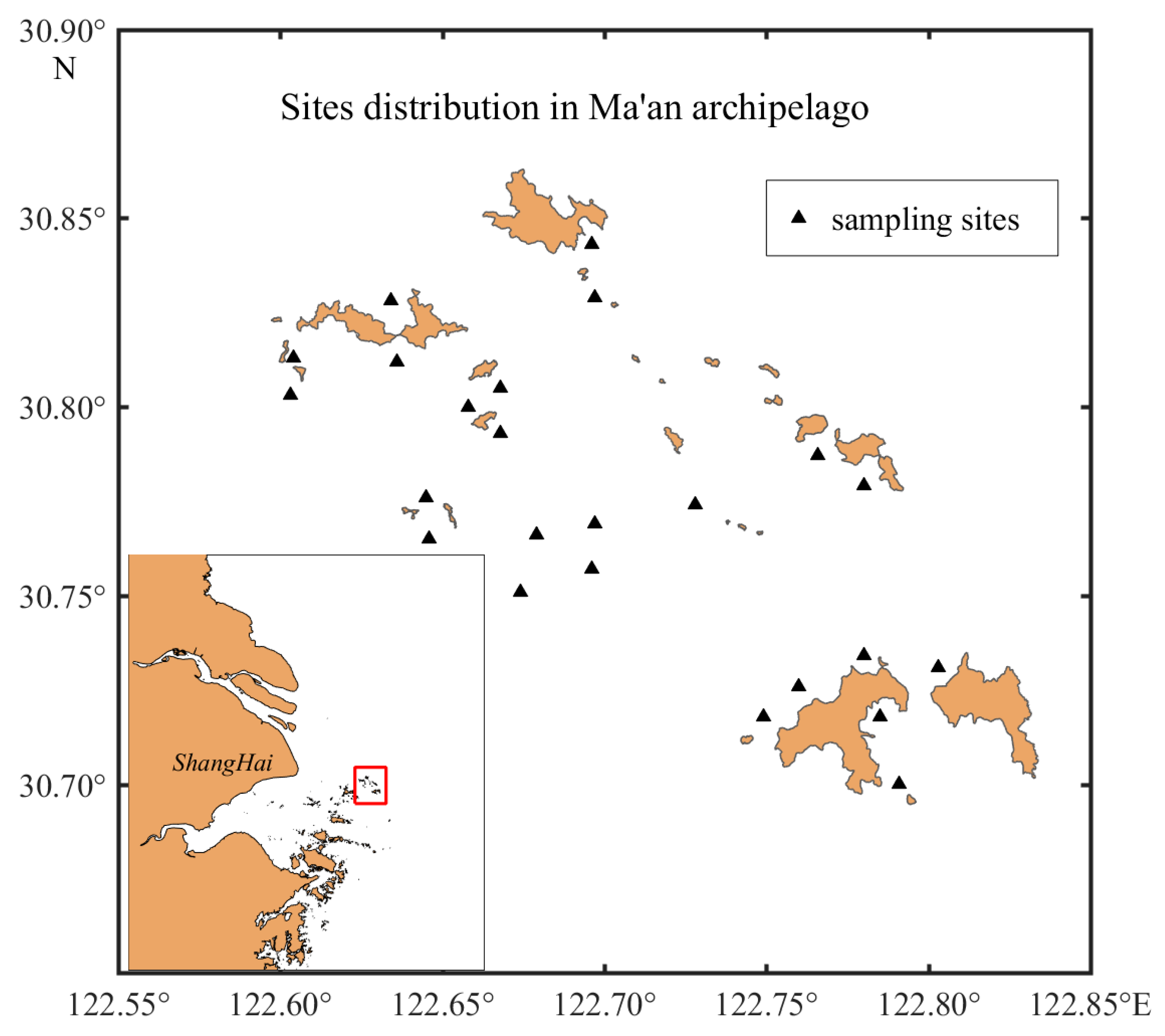
The study area, with a total area of 549 square kilometers, is located at the Ma’an archipelago, Zhejiang province, China (Figure 1). Habitats in this area have large spatial heterogeneity and vary greatly on a rather small spatial scale, which ranges from rock reef, sand, mud, and mussels aquaculture area to other natural or artificial habitats [27]. The water depth in this area ranges from 3 m to more than 30 m.
The fish communities in the study area showed an obvious seasonal time distribution and a uniform spatial distribution. In the rocky reef habitat, which is mainly supported by macro algae, the community structure of living resources changes with the seasonal distribution of macro algae [27]. Dominant species in the near shore rocky area are Sebastiscu smarmoratus, Agrammus and Nibeaalbiflora. Platessapercocephalus, Lateolabrax maculates, and Larimichthys polyactis are common species. The species in the sand habitat, which are mainly Paraplagusia japonica and migration species, such as Thrissa kammalensis and Mugilcephalus, play an important role in the species composition. The species composition in the mud habitat is very different from that in the rocky reef habitat as Johnius belangerii and Lophius litulon are the common species. In the study area, the habitats of mussel aquaculture area and aquaculture cages were very attractive to Hexagrammos otakii and Sebastiscus marmoratus. The species in the artificial reef habitat are mainly reef fish species, such as Sebastiscus marmoratus.
2.3. Data Collection
The data of demersal fish community and environment variables used for modeling were collected monthly during 2009 from 24 sampling sites, which were identified roughly through the stratification based on the habitat types (Figure 2). Data collected in the survey included demersal fish abundance, longitude, latitude, month, temperature, salinity, oxygen, chlorophyll, turbidity, depth, and type of habitats. Two stationary bottom gillnet types were used as the sampling gear because the trawl cannot be used in every type of habitat. One had a height of 1.8 m with four different mesh sizes (25 mm, 34 mm, 43 mm, and 58 mm) and a total length of 60 m. The other set of gillnets were 2.4 m high with mesh sizes of 50 mm, 60 mm, 70 mm, and 80 mm in panels of 30 m length each (a total length of 120 m). Gillnets were set for about 24 h (mean of 23.6 ± 2.5 h) at each sampling site, the data was not transformed to Catch-per-unit-effort since the sampling times were close. The species of each fish sampled was identified and the abundance of each fish species was measured. The sampling location was recorded by GPS (Global Positioning System). The CTD (Conductivity, Temperature and Depth sensor; seabird 19 plus) was used to measure depth, temperature, salinity, chlorophyll, turbidity, and oxygen.
Margalef’s richness index (D) and Shannon index (H’) were chosen to quantify fish communities in the analysis of spatial assemblages of demersal fish species [28]. The relationship between the selected fish community index and environmental variables was developed using a generalized additive model (GAM). Habitats and environmental variables, such as temperature, depth and salinity, play a major role in influencing fish community distribution [29,30]. Different habitats may result in different fish community assemblages [31]. As there is a large spatial heterogeneity in the distribution of habitats in the study area, the type of habitat was chosen as an important variable. Other environmental variables, such as depth, temperature, and salinity, were also important in influencing fish distribution directly or indirectly [32,33,34]. The environmental variables chosen for this study included longitude, latitude, month, temperature, salinity, oxygen, chlorophyll, turbidity, depth, and type of habitats.
PCA-based GAM used a logic link function with a Gaussian error distribution. The GAM for the Margalef’s richness index or Shannon index can be written as:
where Margalef’s richness index is the richness of the demersal fish community; the Shannon index is the diversity of the demersal fish community; Logit is a logit link function; s is the spline smoother; Lon is longitude; Lat is latitude; comp i is the ith principal component, n is the number of principal components chosen to be included in the PCA-based GAM; month ranges from January to December; and type is habitattypes, including rock reef, sand, mud, mud and sand, mussel aquaculture area, artificial reef and aquaculture cage. This PCA-based GAM method was shown to perform better than the original variables-based GAM [28].
Based on the estimated PCA-based GAM model and environmental variables, the spatial distribution of Margalef’s richness index and Shannon index in June, August, October, and September in 2012 and February and April in 2013 were predicted (Figure 3). This predicted spatial distribution of demersal fish community index was considered as the “true” fish community structure in the evaluation of different sampling designs.
2.4. Treatment Sampling Designs
The size of sampling grids used in this study was 300 × 300 m, which was proposed based on the size of the gillnets used in sampling [10]. There were 3381 potential sampling stations of the defined size within the study area. Those stations that were in edges and/or could not be sampled were not included in the 3381 stations. The following four sampling designs were considered in the evaluation:
(1) Simple random sampling
n sites were randomly selected for sampling from the potential 3381 sites. This design was referred to as Design I.
(2) Systematic sampling design
All 3381 sites were sorted by longitude first and then by latitude. The list of all the stations were evenly divided into n groups, before the sampling distance d was calculated as 3381/n. One station was selected from each of the n groups for sampling, resulting in n sites selected for sampling. The first site was chosen randomly from the first group, followed by sites with a sampling distance of d, 2d, … and (n−1)d. This design was referred to as Design II.
(3) Stratified sampling design
A previous study suggests that substrates tended to influence the fish species composition in the study area [27] and we used the substrates to stratify the survey area. Sand and artificial reef take up a small area and thus, they were combined into one stratum. Therefore, four strata were defined based on substrates for the stratified sampling design: rock reef, sand and artificial reef, mud as well as mud and sand. The total number of potential sites for sampling was 139 in the rock-reef stratum; 35 sites in sand and artificial reef; 2339 sites in mud; and 868 sites in mud and sand. Samples were randomly selected within each stratum. The performance of the stratified sampling design can be greatly affected by the allocation of the sampling efforts among the strata [3]. In this study, we considered two sample allocation scenarios for the stratified sampling design:
- (1)
- Allocate samples based on the habitat area proportion of each stratum (referred to as Design III)
- (2)
- Allocate the first half of samples evenly among the strata first, then allocate the remaining samples in a way that is inversely proportional to the variances of strata (Neyman allocation referred to as Design IV).
2.5. Simulation Procedure and Measure Indices
In order to test the impact of sample size on precision, three sample sizes were considered (25, 50 and 100). For a given sample size of each design, we sampled the “true” fish community (Figure 2) 100 times. For each simulated sampling, we calculated three performance indices used in this study to measure the performance of the sampling design: Design effect (Deff), Relative Estimation Error (REE), and Relative Bias (RB) [12,35]. The three indices reflect different aspects of sampling performance. Deff measures the effectiveness of a sampling design relative to the simple random design; REE measures the overall errors of estimated mean; and RB measures the level of estimation bias for a given design. The three indices can be written as:
where Vk() is the variance of sample mean of kth sampling design; VSRS() is the variance of the sample mean derived for the simple random design; Vestimated is the estimated mean in the jth simulation run of the kth sampling design; Vtrue is the true mean of the kth sampling design; and N is the number of simulation runs (i.e., 100).
2.6. The Influence of Temperature Change
In order to assess the influence of temperature on the performance of the sampling design for the distribution, the performance was evaluated with increases in temperature that were uniform or non-uniform [36]. Two scenarios were considered: (1) Temperature did not uniformly increase spatially. The scenario of the non-uniform spatial increase of temperature was simulated with the temperature of a warmer month but all other environmental variables were kept invariant. In this study, February, April, and June were selected. For example, when the community index in February was simulated, the temperature for prediction came from April while keeping the other environmental variables invariant. (2) Temperature in each month increased consistently and uniformly by 1 °C to 5 °C. The distribution of the demersal fish was predicted based on the GAM with the increased temperature. To avoid temperatures beyond the upper limit, the indices for February were selected in this section.
All calculations and simulations were run in R2.15.0 [37].
3. Results
3.1. Design Effect (DEFF)
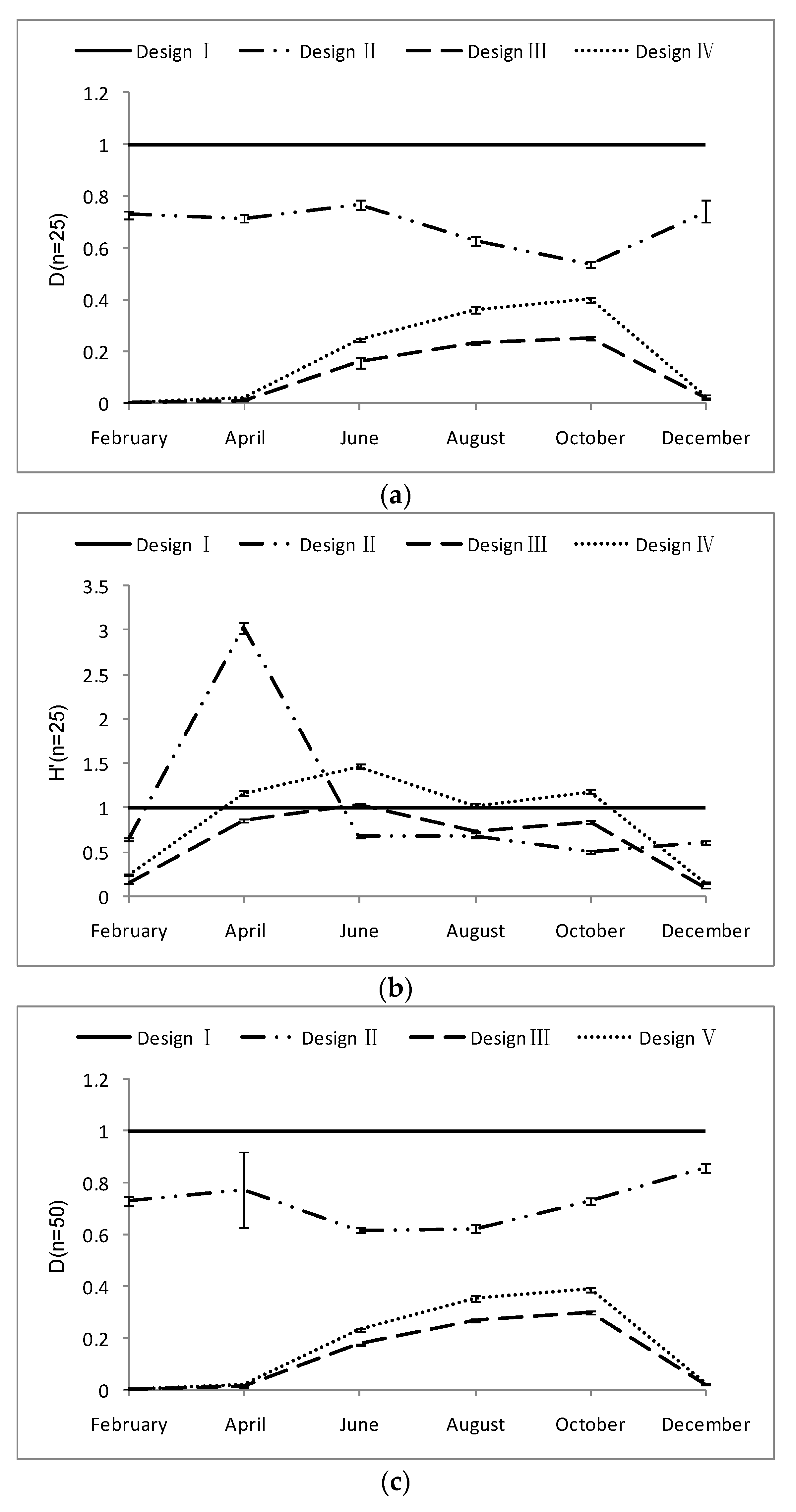
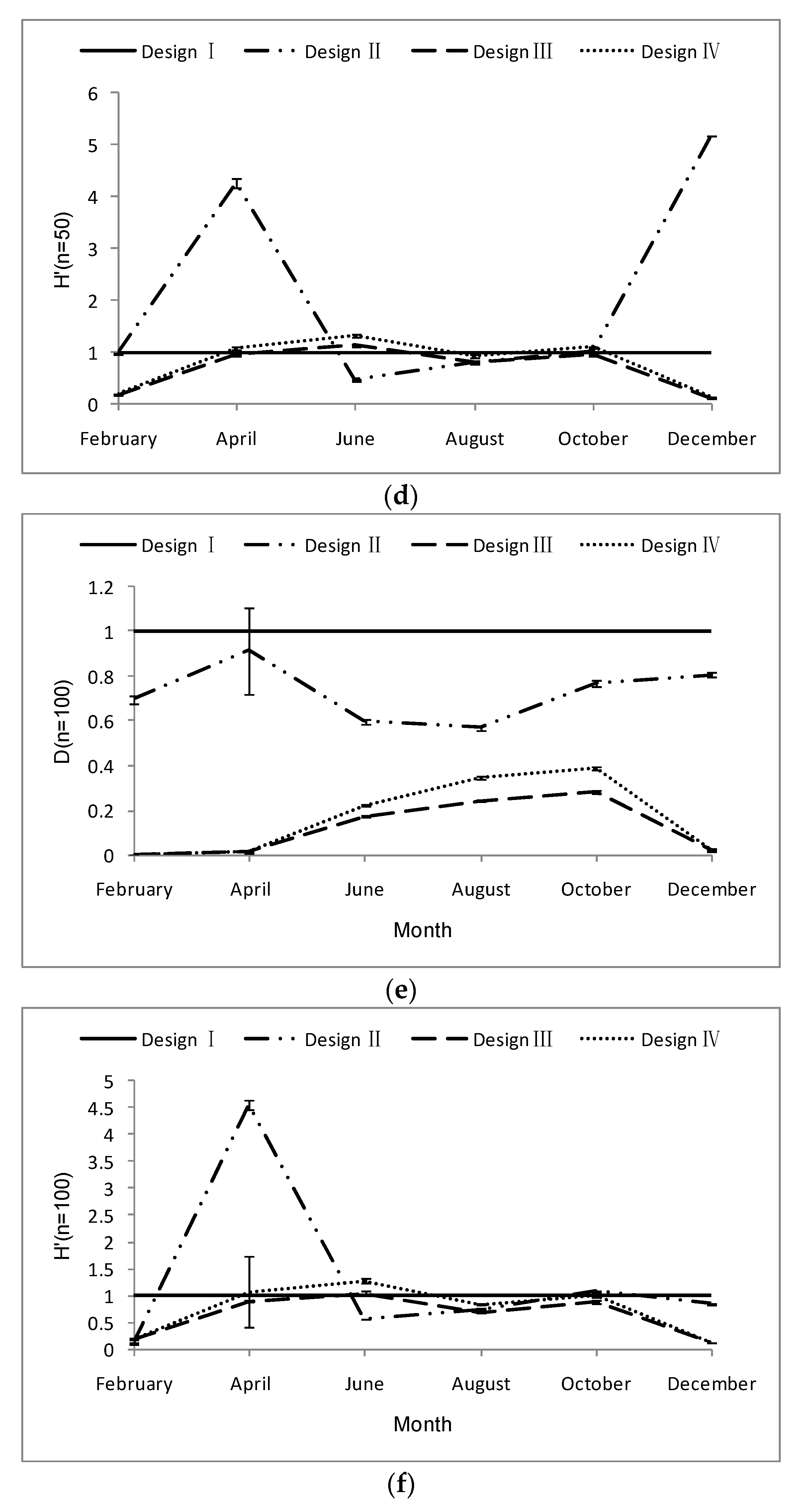
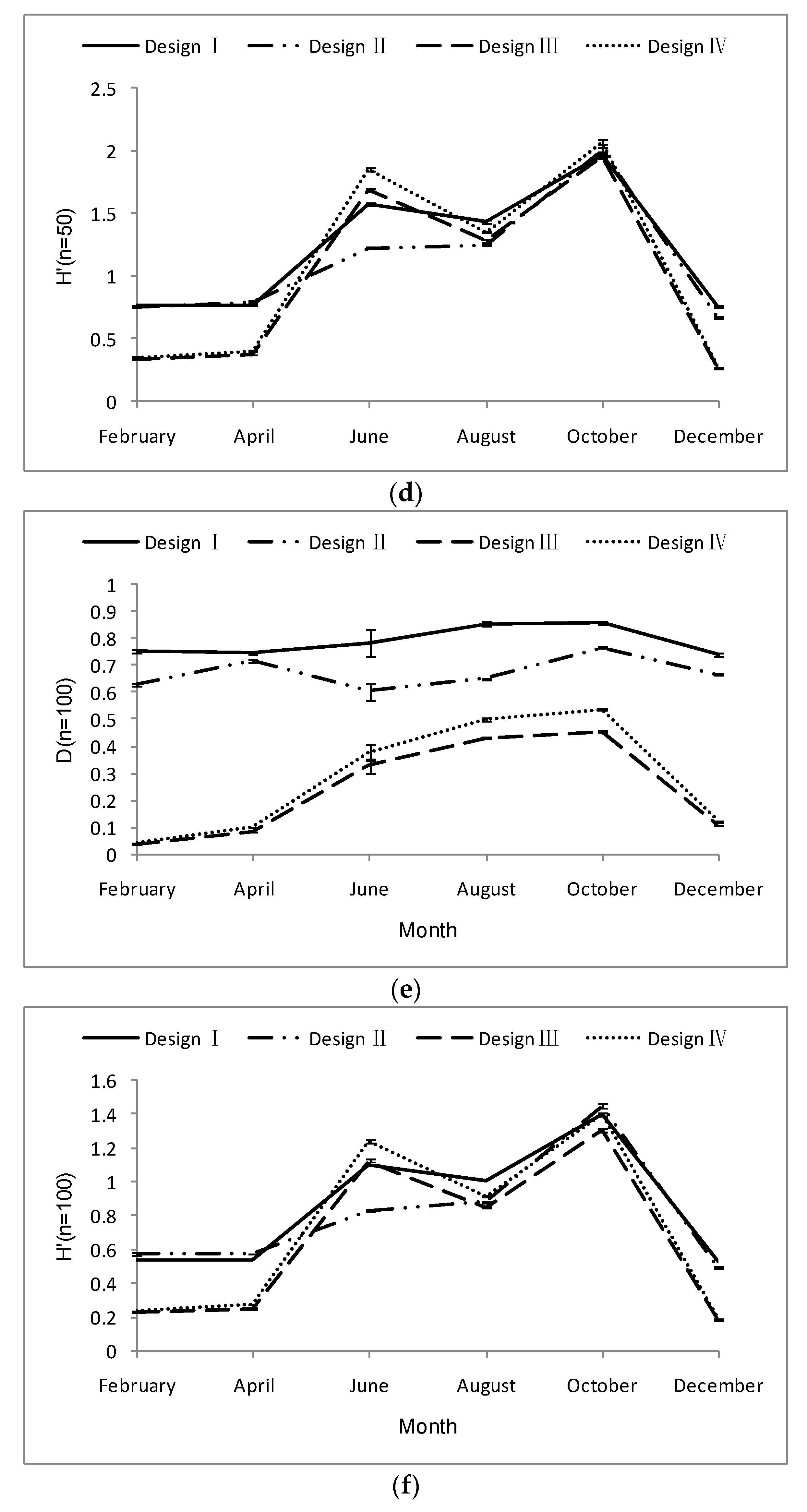
The values of Deff showed that the performance of four sampling designs for the Margalef’s richness index had the following ranking: Design III > Design IV > Design II > Design I (Figure 4a,c,e). Design III performed best in all six months. For the Shannon index, the ranking of designs was: Design III > Design I > Design IV > Design II (Figure 4b,d,f). Design III performed well in the overall average of Deff but did not always perform best in all the 6 months. For example, Design II performed best in June with a sample size of 25 (Figure 4b).
3.2. Relative Estimation Error (REE)
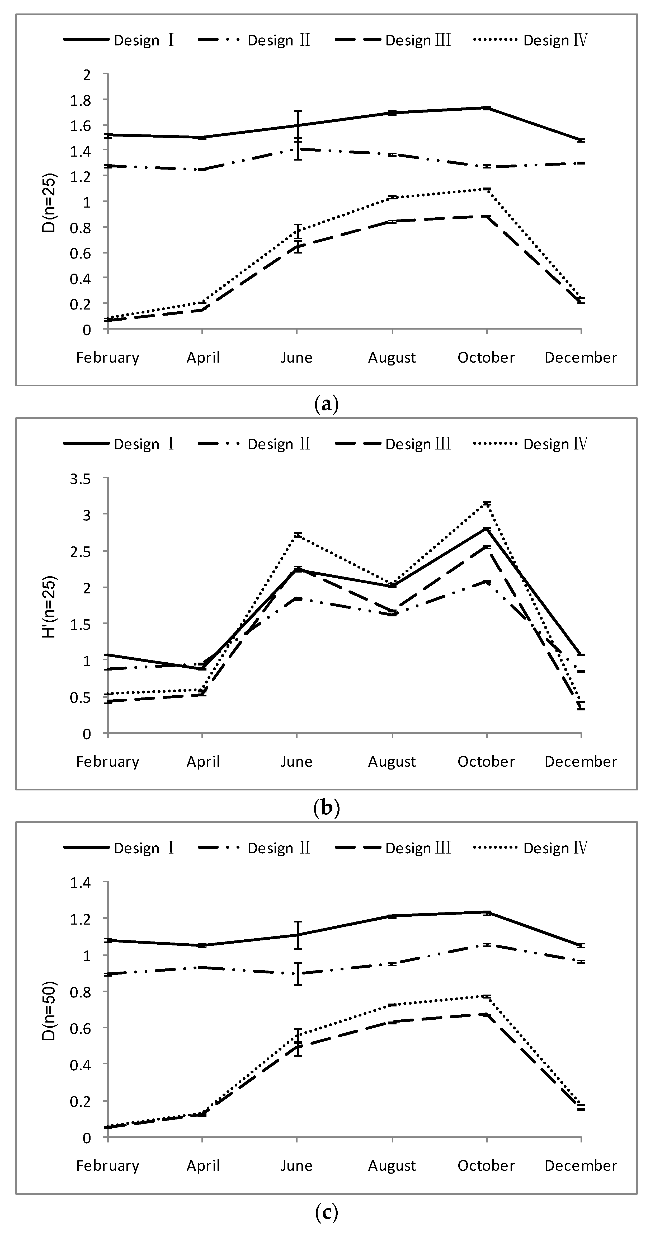
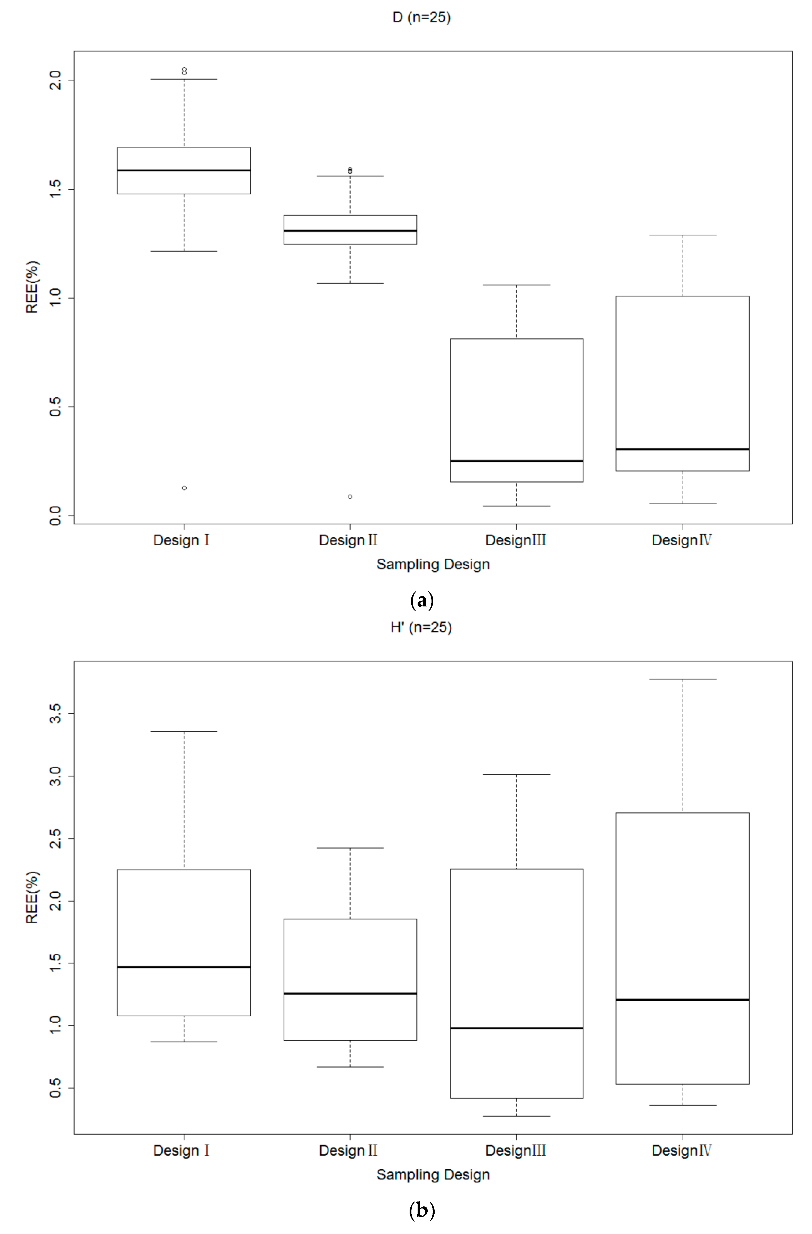
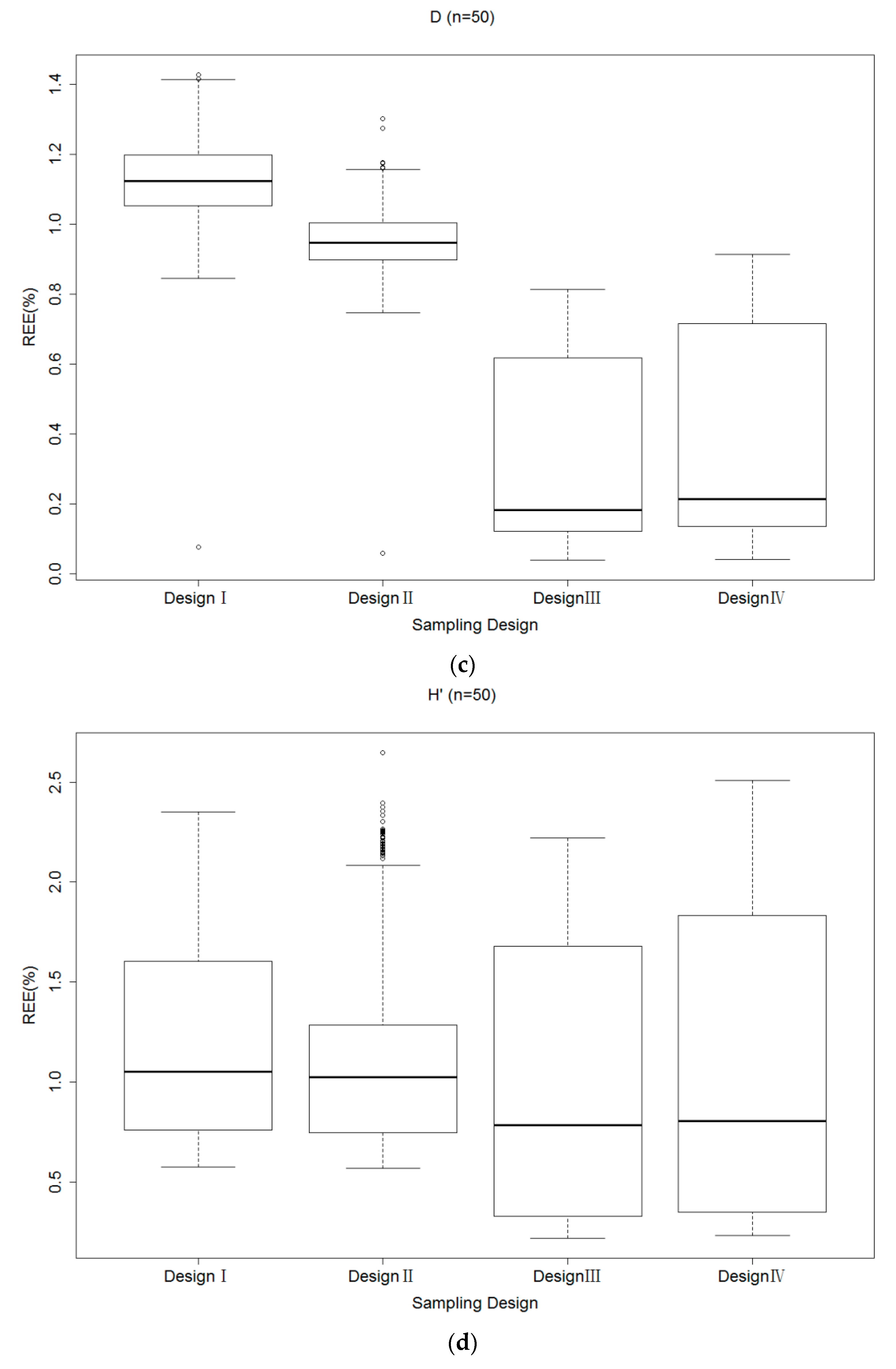
Design III yielded the best estimates of Margalef’s richness index, followed by Design IV. Design I performed the worst for all the three levels of sample sizes considered in this study (Figure 5a,c,e). For example, the average REE was 1.590 (approximately 1.481–1.738) for Design I and 0.470 (0.155–0.890) for Design III. The REE of stratified sampling design was smaller than that for the systematic sampling design and simple random sampling (Figure 6).
3.3. Relative Bias (RB) of Each Sampling Design
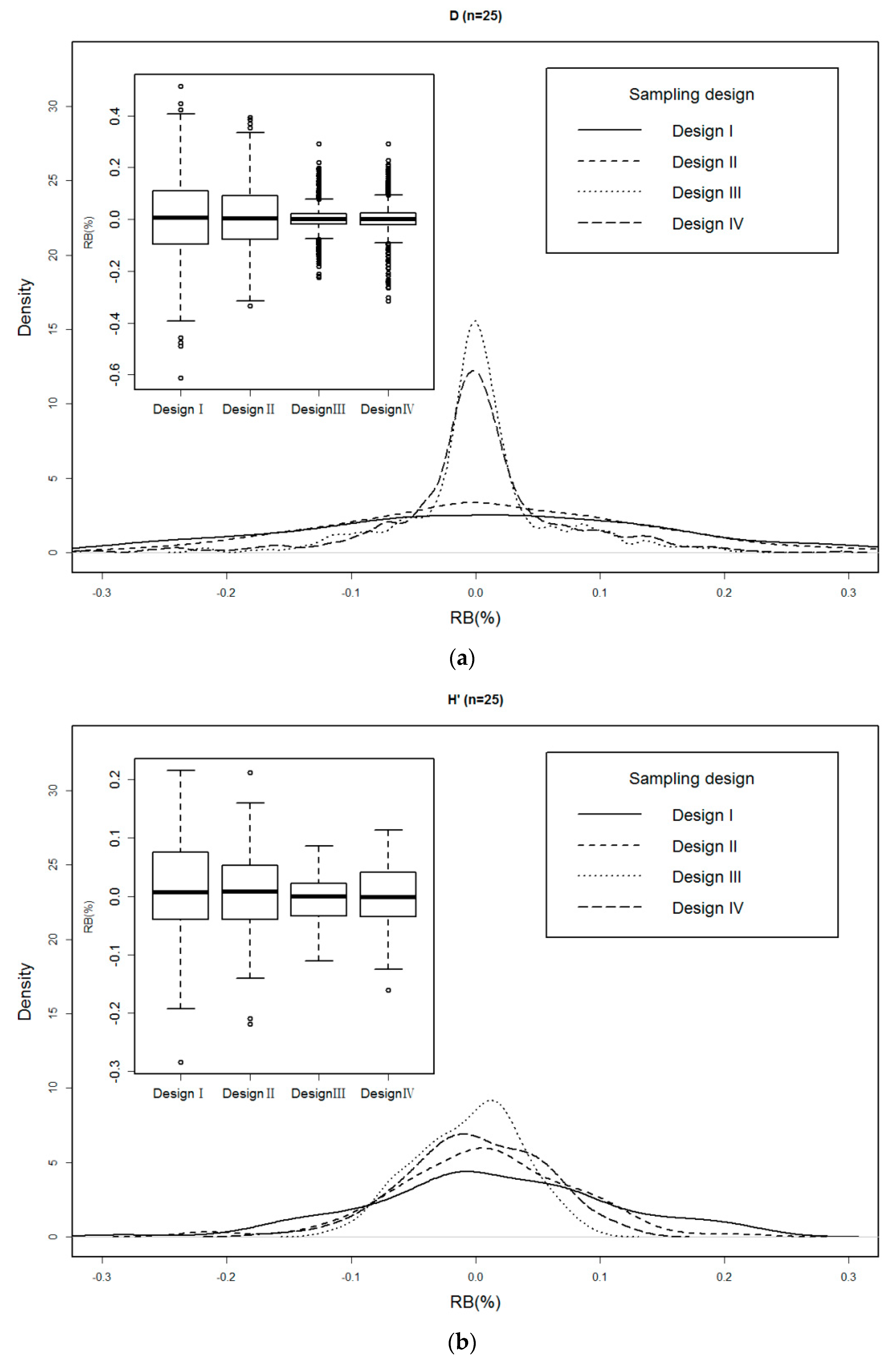
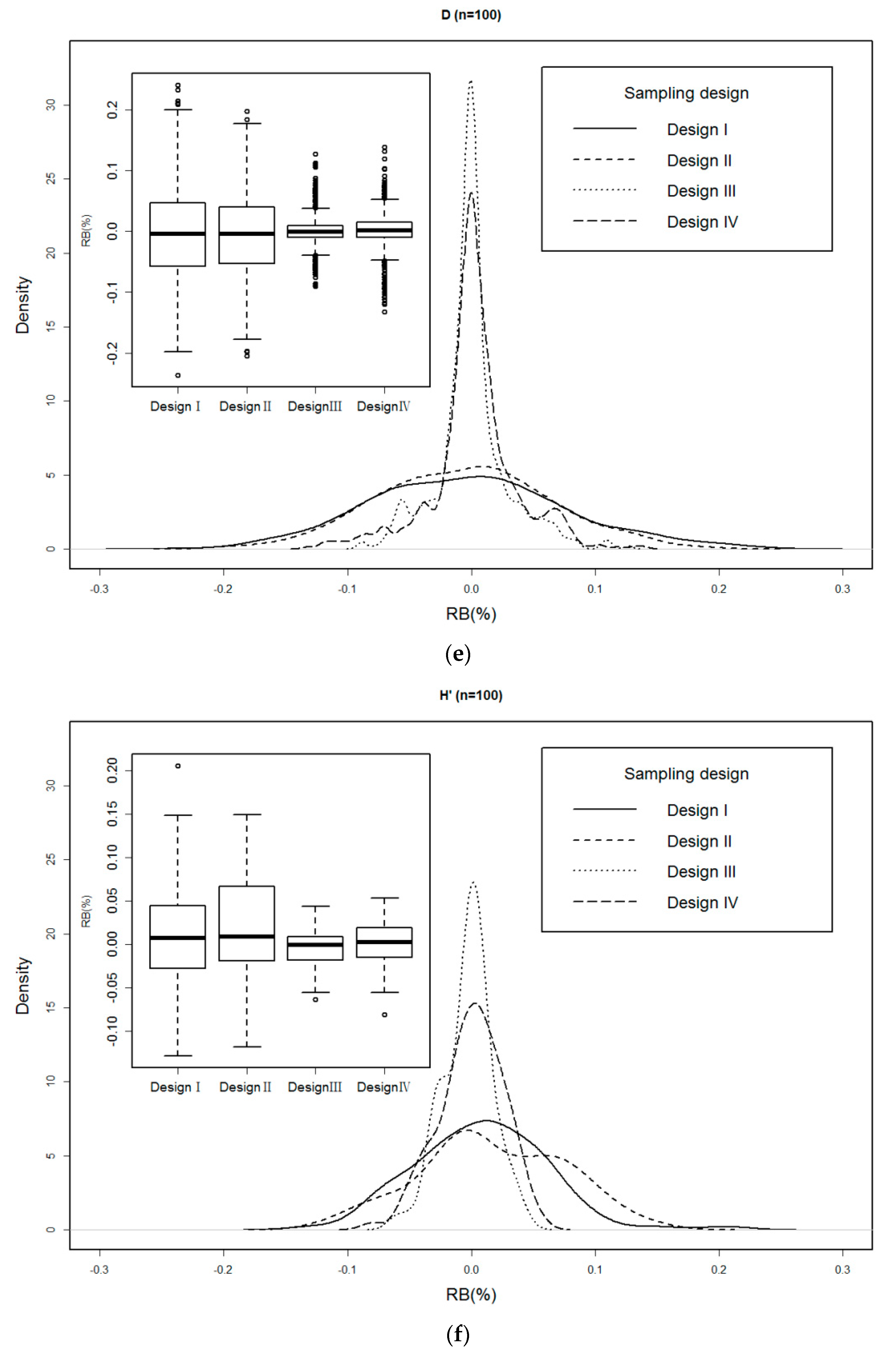
For the Margalef’s richness index, RB values of the four sampling designs were distributed symmetrically around 0 (Figure 7a,c,e), indicating that all the designs yielded more or less unbiased estimates. The distribution of RB was narrower and more concentrated for the stratified sampling design than that for the simple random sampling design and systemic sampling design. There was no obvious difference in the RB between the two stratified sampling designs (i.e., Designs III and IV).
For the Shannon index, the RB values of the four sampling designs were not distributed symmetrically around 0. For example, Design II was skewed with a distribution tail extending to the right when the sample size was 50, suggesting that the systematic sampling design might overestimate the Shannon index. Stratified sampling designs (Design III and Design IV) yielded similar distributions for the Margalef’s richness index and Shannon index (−0.1 to 0.1). However, the distributions of Design I and Design II for the Margalef’s richness index (−0.2 to 0.2) was wider than the Shannon index (−0.1 to 0.1). The range of the RB distribution decreased and became closer to 0 for all four designs when the sample sizes increased from 25 to 100 (Figure 7).
3.4. Possible Influence of Temperaturechanges
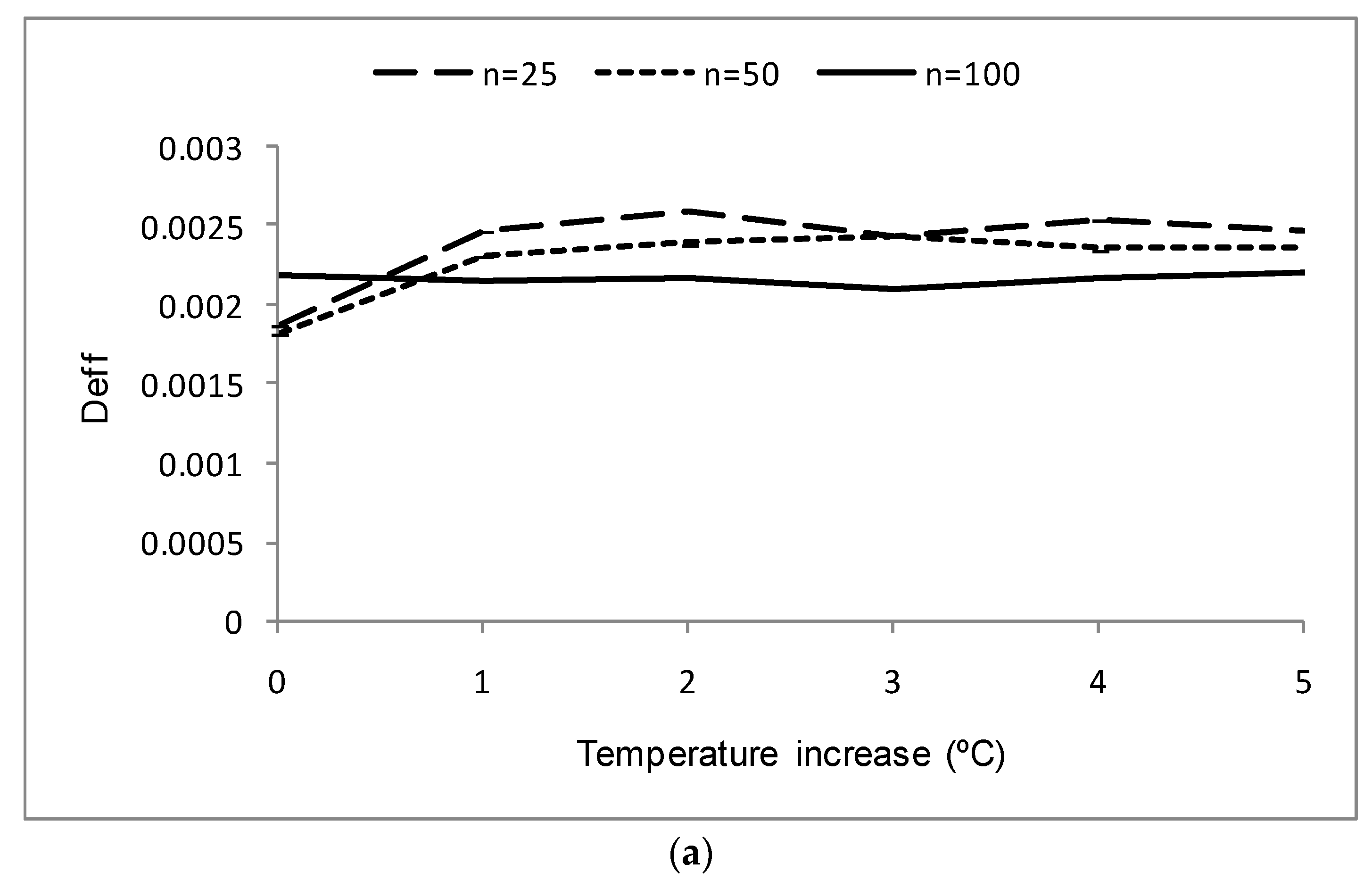
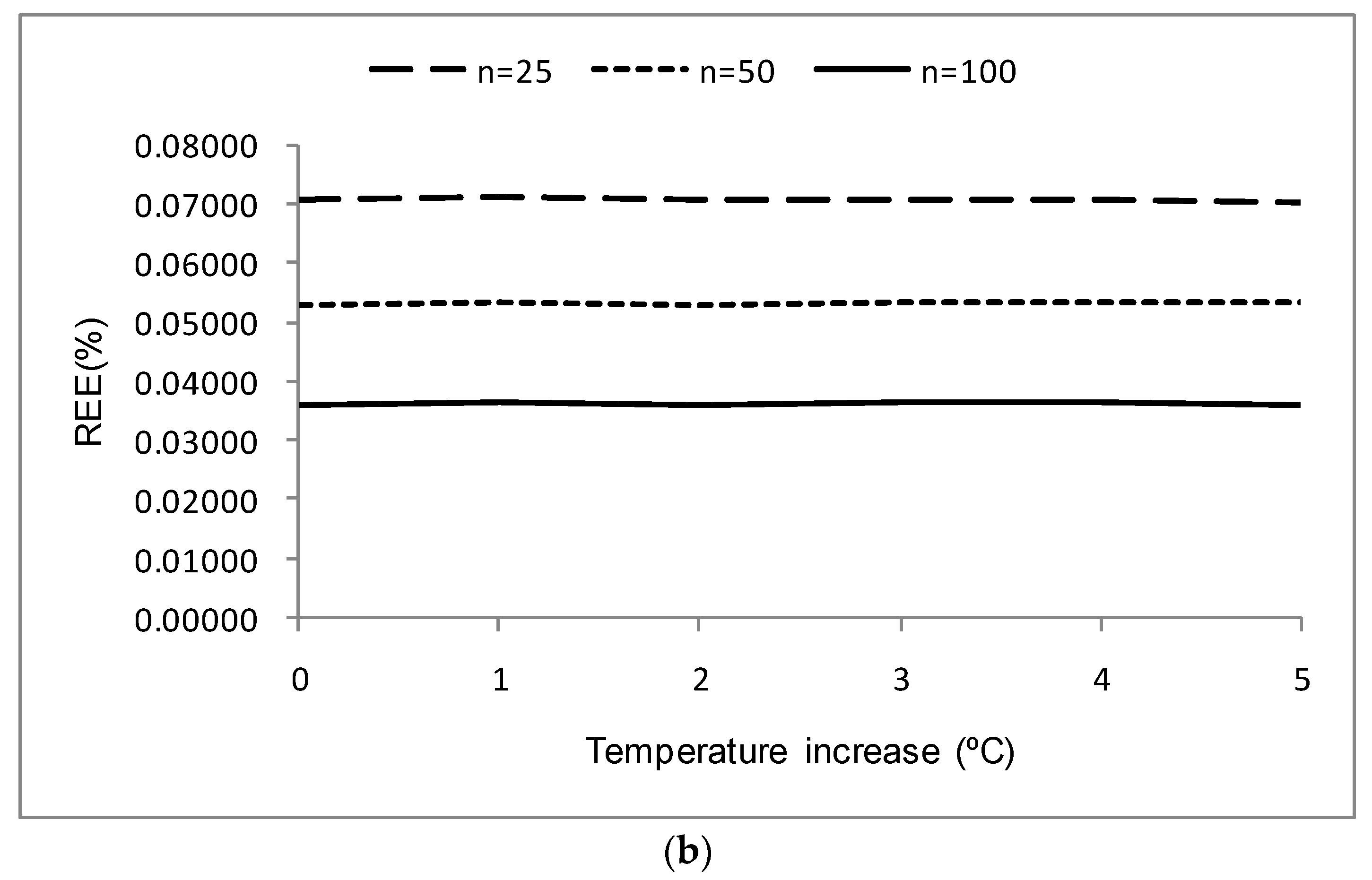
When the temperature uniformly increased across the study area by 1–5 °C, Design III performed well because it had the lowest Deff and REE among the four sampling designs (Table 1). With an increased temperature, the Deff and REE of Design III did not change much (Figure 8). Because the same result was obtained for the Shannon index, only the Margalef’s richness indexis shown in Figure 8.
When the temperature increased non-uniformly across the study area, Design II had the lowest REE (Table 2). However, the Deff of Design II was not the best. The values of Deff for the four sampling designs had the following ranking: Design III > Design IV > Design II > Design I.
4. Discussion and Conclusions
The performance of different sampling designs in estimating fish abundance was examined in many studies [2,7,9,38]. Most of these studies focused on the population of a single fish species [7], while only a few studies focused on the fish communities. There is a lack of research evaluating the influence of temperature change on the performance of a sampling design. In this study, the four sampling designs were compared in their performance of estimating different community structure indices, while the influence of temperature change on sampling was also evaluated. This study shows that a stratified sampling design (Design III) yielded the best estimates. However, the performance of Design III might vary with increased temperature.
All sampling designs have their advantages and disadvantages [39,40]. A systemic sampling design can be easily operated and is more suitable for sampling fish communities with no prior information [3,41]. A stratified random sampling design is also commonly used in many fishery surveys [2,12,15] and the variance between strata can be reduced by suitable stratification. Previous studies have shown that a systemic sampling design and stratified sampling design tend to have higher accuracy than simple random sampling [16,42]. For an infinite population, a stratified sampling design with equally sized stratum has higher precision [2,16]. The distribution of fish community indices showed a large spatial variability as a result of the patchy distribution of various habitats. The stratified sampling design (Design III) tested in this study is based on substrate types for the stratification and thus reduces the variance between strata and improves the precision of the estimates.
The stratified sampling design based on strata area (i.e., Design III) performed best out of the two stratified sampling designs. For a stratified sampling design, the allocation of sampling efforts can be done using several different criteria [2,12]. Neyman allocation allocates samples based on strata variance [43]. However, it is difficult to know the variance before a survey is conducted or during the survey. In general, previous years’ surveys can be used to estimate the variance [3,43]. In this study, as the sampling area is not very large, it is possible to do a Neyman allocation based on an initial equal samples allocation first. However, it is more suitable to use the variance estimated from previous years’ surveys when the sample areas are large or the environment has changed greatly. In this study, Design III, which allocates sampling efforts among the strata based on strata areas, tends to perform better than the Design IV based on the Neyman allocation, although the difference is small (Figure 2, Figure 3 and Figure 5). Proportional allocation of stratified sampling design was relatively simple without the requirement of previous knowledge on spatial variability in organism distributions, which is required in the Neyman allocation [12].
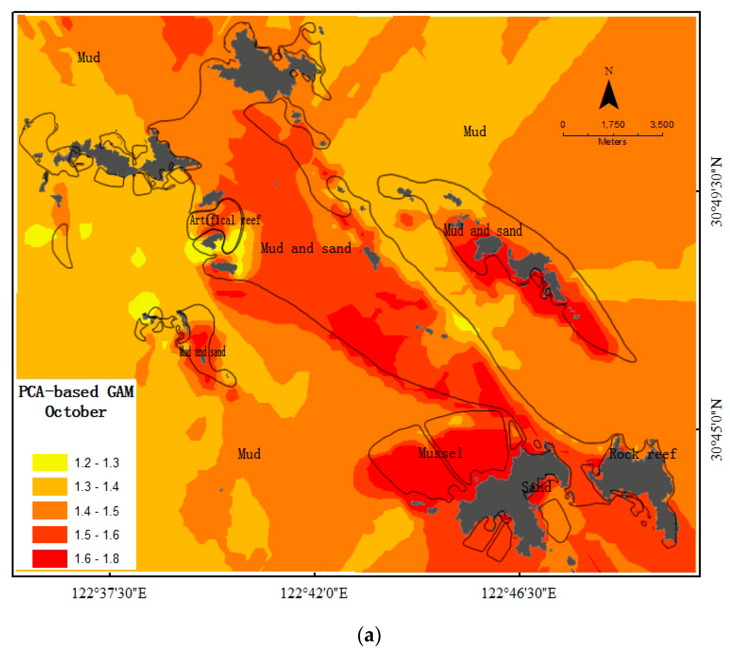
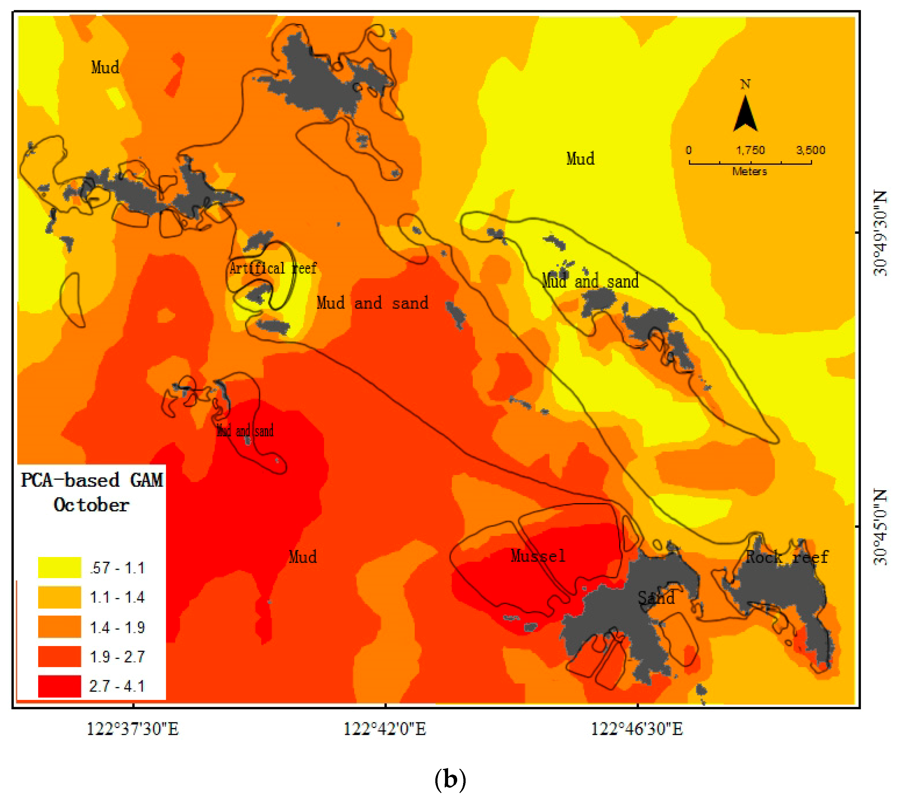
The choice of optimal sampling design may depend on the objectives of a sampling program [39]. Traditional sampling designs, such as systemic sampling design and stratified sampling design, were more suitable for a continuous distribution or area source occupying large spatial areas [3]. As we used the fish community indices in this study instead of the abundance indices of a single fish population, the heterogeneity of the spatial distribution of the fish community was reduced in the whole area. For such cases, the traditional sampling designs are more suitable. The performance of sampling designs was different between the Margalef’s richness index and the Shannon index. For example, Design III had the smallest REE in all the months for the Margalef’s richness index, but this was not true for the Shannon index. This might result from the different spatial distribution of these two indices [7], the Margalef’s richness index yielded more regular and obvious patterns between different habitats than the Shannon index (Figure 2). The strata of the stratified sampling design were decided by habitat types. Thus, the estimation errors of stratified sampling design were higher for the Margalef’s richness index than for the Shannon index.
Design III performed best when the temperature was predicted to increase uniformly over the study area. The trend of the four sampling designs changed inconspicuously with an increase of 5 °C in temperature. The Deff and REE values of Design III were still at the same level with the changes in temperature (Figure 6). This may result from the fact that the modeled temperature change did not result in large changes in the spatial distribution of the synthetic fish community indices. In this study, although the values of richness or diversity indices changed, the spatial pattern was not significantly change. Thus, a uniform change in temperature across the study area resulted in almost no changes in the ranking of the performance of the sampling design.
Design II performed better when the temperature increased non-uniformly. Design III was not the optimal sampling design, although Deff was the smallest. Under this temperature change scenario, Design III performed worse than in the unaltered temperature (Figure 5, Table 2). This may result from the large changes in the spatial distribution of fish community indices as a result of non-uniform changes in the habitats. Thus, the stratification based on previous habitat did not perform well. It is important to adjust the strata for the stratified sampling design when the habitat experiences large changes in the target area. This suggests that we need to carefully evaluate the appropriateness of stratification when temperature change-induced habitat changes are large enough to result in substantial changes to a fish community.
Sample size was an important factor affecting the precision of indices from the sampling designs [44]. The influence of sample size was examined in this study with the sample sizes increasing from 25 to 100. In some cases, optimal sampling design can improve the precision resulting from a low sampling effort. For example, Design III with a sample size of 25 is more accurate than the simple random sampling (Design I) with a sample size of 50 (Figure 5). The simple random sampling with a sample size of 100 has the same estimation accuracy as the stratified sampling design with a sample size of 25. This suggests that an optimal sampling design can increase sampling accuracy even with a low sampling effort.
A significant relationship was found between fish community and habitats. The optimal sampling design in complicated habitats mainly considers the sampling method and site allocation. This study provided a frame for optimal sampling design chosen for complicated habitats. The ecological model was used first to establish the relationship between the fish community and the environment, especially habitats. The fish community distribution in different habitats can be predicted by this model to be the “true” population for the sampling design. Different sampling design and sampling effort allocation can be compared based on this “true” distribution. Stratified sampling design with sampling effort allocated by habitat area was the optimal sampling designand therefore the stratified sampling design can be used in this water area for a fish community survey. A similar approach used in this study can also be used for other fish species or populations to carry out a fishery-independent survey program.
Fish resources are limited and thus optimal sampling designs are important for fish community protection and utilization. This study evaluated the performance of the four sampling designs for quantifying demersal fish diversity and richness and provided a method for sample design chosen that can be applied to the monitoring of fisheries resources. This study also suggests that we need to carefully evaluate the appropriateness of stratification when the temperature change-induced habitat changes are large enough to result in substantial changes to a fish community.
Author Contributions
Conceptualization, J.Z. and S.Z.; Methodology, J.Z., Y.C. and J.C.; Software, J.Z. and J.C.; Validation, Y.C. and S.Z.; Formal analysis, J.Z. and S.T.; Resources, S.Z.; Data Curation, J.Z.; Writing—Original Draft Preparation, J.Z. and S.Z.; Writing—Review and Editing, J.Z. and Y.C.; Visualization, J.Z.; Supervision, S.Z.; Project Administration, J.Z. and S.Z.; and Funding Acquisition, J.Z. and S.Z.
Funding
This research was supported by the National Natural Science Foundation of China (No. 41606146), National Natural Science Foundation of China (No. 41406153), National Natural Science Foundation of China (No. 41176110), Shanghai First-Class Program (Fisheries) Shanghai Ocean University College of Marine Sciences and International Center for Marine Sciences.
Acknowledgments
Data analysis and manuscript writing performed at the University of Maine was partially supported by the Maine Sea Grant College Program. In particular, we would like to thank Zhao Xu and Chen Liangran for their assistance in the field.
Conflicts of Interest
The authors declare no conflict of interest.
References
- Agboola, J.I.; Uchimiya, M.; Kudo, I.; Osawa, M.; Kido, K. Seasonality and environmental drivers of biological productivity on the western Hokkaido coast, Ishikari Bay, Japan. Estuar. Coast. Shelf Sci. 2013, 127, 12–13. [Google Scholar] [CrossRef]
- Ault, J.S.; Diaz, G.A.; Smith, S.G.; Luo, J.G. An efficient Sampling survey design to estimate pink shrimp population abundance in Biscayne Bay, Florida. N. Am. J. Fish. Manag. 1999, 19, 696–712. [Google Scholar] [CrossRef]
- Barbraud, C.; Rolland, V.; Jenouvrier, S.; Nevoux, M.; Delord, K.; Weimerskirch, H. Effects of climate change and fisheries bycatch on Southern Ocean seabirds: A review. Mar. Ecol. Prog. Ser. 2012, 454, 285–307. [Google Scholar] [CrossRef]
- Bazigos, G.; Kavadas, S. Optimal sampling designs for large-scale fishery sample surveys in Greece. Mediterr. Mar. Sci. 2007, 8, 65–82. [Google Scholar] [CrossRef]
- Bonvechio, K.I. Determining electric fishing sample size for monitoring fish communities in three Florida lakes. Fish. Manag. Ecol. 2009, 16, 409–412. [Google Scholar] [CrossRef]
- Cabral, H.N.; Murta, A.G. Effect of sampling design on abundance estimates of benthic invertebrates in environmental monitoring studies. Mar. Ecol. Prog. Ser. 2004, 276, 19–24. [Google Scholar] [CrossRef] [Green Version]
- Cao, J.; Chen, Y.; Chang, J.H.; Chen, X.J. An evaluation of an inshore bottom trawl survey design for American lobster (Homarusamericanus) using computer simulations. J. Northwest Atl. Fish. Sci. 2014, 46, 27–39. [Google Scholar] [CrossRef]
- Chen, Y. A Monte Carlo study on impacts of the size of subsample catch on estimation of fish stock parameters. Fish. Res. 1996, 26, 207–223. [Google Scholar] [CrossRef]
- Cochran, W.G. Sampling Techniques, 3rd ed.; John Wiley and Sons: New York, NY, USA, 1977; 900p. [Google Scholar]
- Dorner, B.; Holt, K.R.; Peterman, R.M.; Jordan, C.; Larsen, D.P.; Olsen, A.R.; Abdul-Aziz, O.I. Evaluating alternative methods for monitoring and estimating responses of salmon productivity in the North Pacific to future climate change and other processes: A simulation study. Fish. Res. 2013, 147, 10–23. [Google Scholar] [CrossRef]
- Folmer, O.; Pennington, M. A statistical evaluation of the design and precision of the shrimp trawl survey off West Greenland. Fish. Res. 2000, 49, 165–178. [Google Scholar] [CrossRef]
- Gavaris, S.; Smith, S.J. Effect of allocation and stratification strategies on precision of survey abundance estimates for Atlantic Cod (Gadusmorhua) on the eastern Scotian shelf. J. Northwest Atl. Fish. Sci. 1987, 7, 137–144. [Google Scholar] [CrossRef]
- Giri, S.; Mukhopadhyay, A.; Hazra, S.; Roy, D.; Ghosh, S.; Ghosh, T.; Mitra, D. A study on abundance and distribution of mangrove species in Indian Sundarban using remote sensing technique. J. Northwest Atl. Fish. Sci. 2014, 4, 359–367. [Google Scholar] [CrossRef]
- Gray, C.A. Evaluation of fishery-dependent sampling strategies for monitoring a small-scale beach clam fishery. Fish. Res. 2016, 177, 24–30. [Google Scholar] [CrossRef]
- Irvine, G.V.; Shelly, A. Sampling design for long-term regional trends in marine rocky intertidal communities. Environ. Monit. Assess. 2013, 185, 6963–6987. [Google Scholar] [CrossRef] [PubMed]
- Jaureguizar, A.J.; Menni, R.; Guerrero, R.; Lastan, C. Environmental factors structuring fish communities of the Río de la Plata estuary. Fish. Res. 2004, 66, 195–211. [Google Scholar] [CrossRef]
- Jenkins, G.P.; Wheatley, M.J. The influence of habitat structure on nearshore fish assemblages in a southern Australian embayment: Comparison of shallow seagrass, reef-algal and unvegetated sand habitats, with emphasis on their importance to recruitment. J. Exp. Mar. Biol. Ecol. 1998, 221, 147–172. [Google Scholar] [CrossRef]
- Johnston, R.; Sheaves, M.; Molony, B. Are distributions of fishes in tropical estuaries influenced by turbidity over small spatial scales? J. Fish Biol. 2007, 71, 657–671. [Google Scholar] [CrossRef]
- Kodama, K.; Aoki, I.; Shimizu, M.; Taniuchi, T. Long-term changes in the assemblage of demersal fishes and invertebrates in relation to environmental variations in Tokyo Bay, Japan. Fish. Manag. Ecol. 2002, 9, 303–313. [Google Scholar] [CrossRef]
- Liu, Y.; Chen, Y.; Cheng, J. A comparative study of optimization methods and conventional methods for sampling design in fishery-independent surveys. ICES J. Mar. Sci. 2009, 66, 1873–1882. [Google Scholar] [CrossRef] [Green Version]
- Liu, C.; White, M.; Newell, G.; Griffioen, P. Species distribution modeling for conservation planning in Victoria, Australia. Ecol. Model. 2013, 249, 68–74. [Google Scholar] [CrossRef]
- Loeng, H. The influence of temperature on some fish population parameters in the Barents Sea. J. Northwest Atl. Fish. Sci. 1989, 9, 103–113. [Google Scholar] [CrossRef]
- Lohr, S.L. Sampling: Design and Analysis; Duxbury: Pacific Grove, CA, USA, 1999. [Google Scholar]
- Lopez-Lopez, L.; Preciado, I.; Velasco, F.; Olaso, I.; Gutiérrez-Zabala, J.L. Resource partitioning amongst five coexisting species of gurnards (Scorpaeniforme: Triglidae): Role of trophic and habitat segregation. J. Sea Res. 2011, 66, 58–68. [Google Scholar] [CrossRef]
- Maes, J.; Stevens, M.; Breine, J. Modelling the migration opportunities of diadromous fish species along a gradient of dissolved oxygen concentration in a European tidal watershed. Estuar. Coast. Shelf Sci. 2007, 75, 1–12. [Google Scholar] [CrossRef]
- Manly, B.F.J.; Akroyd, J.M.; Walshe, K.A.R. Two-phase stratified random surveys on multiple populations at multiple locations. N. Z. J. Mar. Freshw. Res. 2002, 36, 581–591. [Google Scholar] [CrossRef]
- Masia, A.; Iskander, M.; Negm, A. Coastal protection measures, case study (Mediterranean zone, Egypt). J. Coast. Conserv. 2015, 3, 281–294. [Google Scholar] [CrossRef]
- Parmesan, C. Ecological and evolutionary responses to recent climate change. Annu. Rev. Ecol. Syst. 2006, 37, 637–669. [Google Scholar] [CrossRef]
- Pennington, M.; Vølstad, J.H. Optimum size of sampling unit for estimating the density of marine populations. Biometrics 1991, 47, 717–723. [Google Scholar] [CrossRef]
- Pinheiro, H.T.; Martins, A.S.; Joyeux, J.C. The importance of small-scale environment factors to community structure patterns of tropical rocky reef fish. J. Mar. Biol. Assoc. UK 2013, 93, 1175–1185. [Google Scholar] [CrossRef]
- Pooler, P.S.; Smith, D.R. Optimal sampling design for estimating spatial distribution and abundance of a freshwater mussel population. J. N. Am. Benthol. Soc. 2005, 24, 525–537. [Google Scholar] [CrossRef]
- R Development Core Team. R: A Language and Environment for Statistical Computing; R Foundation for Statistical Computing: Vienna, Austria, 2016. [Google Scholar]
- Ripley, B.D. Spatial Statistics; John Wiley and Sons: New York, NY, USA, 1981; 252p. [Google Scholar]
- Skibo, K.M.; Schwarz, C.J.; Peterman, R.M. Evaluation of sampling designs for red sea urchins Strongylocentrotus franciscanus in British Columbia. N. Am. J. Fish. Manag. 2008, 28, 219–230. [Google Scholar] [CrossRef]
- Simmonds, E.J.; Fryer, R.J. Which are better, random or systematic acoustic surveys? A simulation using North Sea herring as an example. ICES J. Mar. Sci. 1996, 53, 39–50. [Google Scholar] [CrossRef] [Green Version]
- Simth, S.G.; Ault, J.S.; Bohnsack, J.A.; Harper, D.E.; Luo, J.G.; McClellan, D.B. Multispecies survey design for assessing reef-fish stocks, spatially explicit management performance, and ecosystem condition. Fish. Res. 2011, 109, 25–41. [Google Scholar] [CrossRef]
- Sobocinski, K.L.; Orth, R.J.; Fabrizio, M.C.; Latour, R.J. Historical comparison of fish community structure in lower Chesapeake bay seagrass habitats. Estuar. Coast. 2013, 36, 775–794. [Google Scholar] [CrossRef]
- Somerton, D.A.; McConnaughey, R.A.; Intelmann, S.S. Evaluating the use of acoustic bottom typing to inform models of bottom trawl sampling efficiency. Fish. Res. 2017, 185, 14–16. [Google Scholar] [CrossRef]
- Stein, A.; Ettema, C. An overview of spatial sampling procedures and experimental design of spatial studies for ecosystem comparisons. Agric. Ecosyst. Environ. 2003, 94, 31–47. [Google Scholar] [CrossRef]
- Stokesbury, K.D.E. Estimation of sea scallop abundance in closed areas of Georges Bank, USA. Trans. Am. Fish. Soc. 2002, 131, 1081–1092. [Google Scholar] [CrossRef]
- Wang, Z.H.; Zhang, S.Y.; Chen, Q.M.; Xu, M.; Wang, K. Fish community ecology in rocky reef habitat of Ma’an Archipelago. I. Species compositon and diversity. Biodivers. Sci. 2012, 20, 41–50. (In Chinese) [Google Scholar]
- Xu, B.D.; Ren, Y.P.; Chen, Y.; Xue, Y.; Zhang, C.L.; Wan, R. Optimization of stratification scheme for a fishery-independent survey with multiple objectives. Acta Oceanol. Sin. 2015, 34, 154–169. [Google Scholar] [CrossRef]
- Yu, H.; Jiao, Y.; Su, Z.; Reid, K. Performance comparison of traditional sampling designs and adaptive sampling designs for fishery-independent surveys: A simulation study. Fish. Res. 2012, 113, 173–181. [Google Scholar] [CrossRef]
- Zhao, J.; Cao, J.; Tian, S.Q.; Chen, Y.; Zhang, S.Y.; Wang, Z.H.; Zhou, X.J. A comparison of two GAM models in quantifying relationships of environmental variables and fish richness and diversity indices. Aquat. Ecol. 2013, 48, 297–312. [Google Scholar] [CrossRef]
Figure 1.
Flowchart of the “true” population derived from the principal component analysis based generalized additive model (principal component analysis (PCA)-based generalized additive model (GAM)).
Figure 1.
Flowchart of the “true” population derived from the principal component analysis based generalized additive model (principal component analysis (PCA)-based generalized additive model (GAM)).
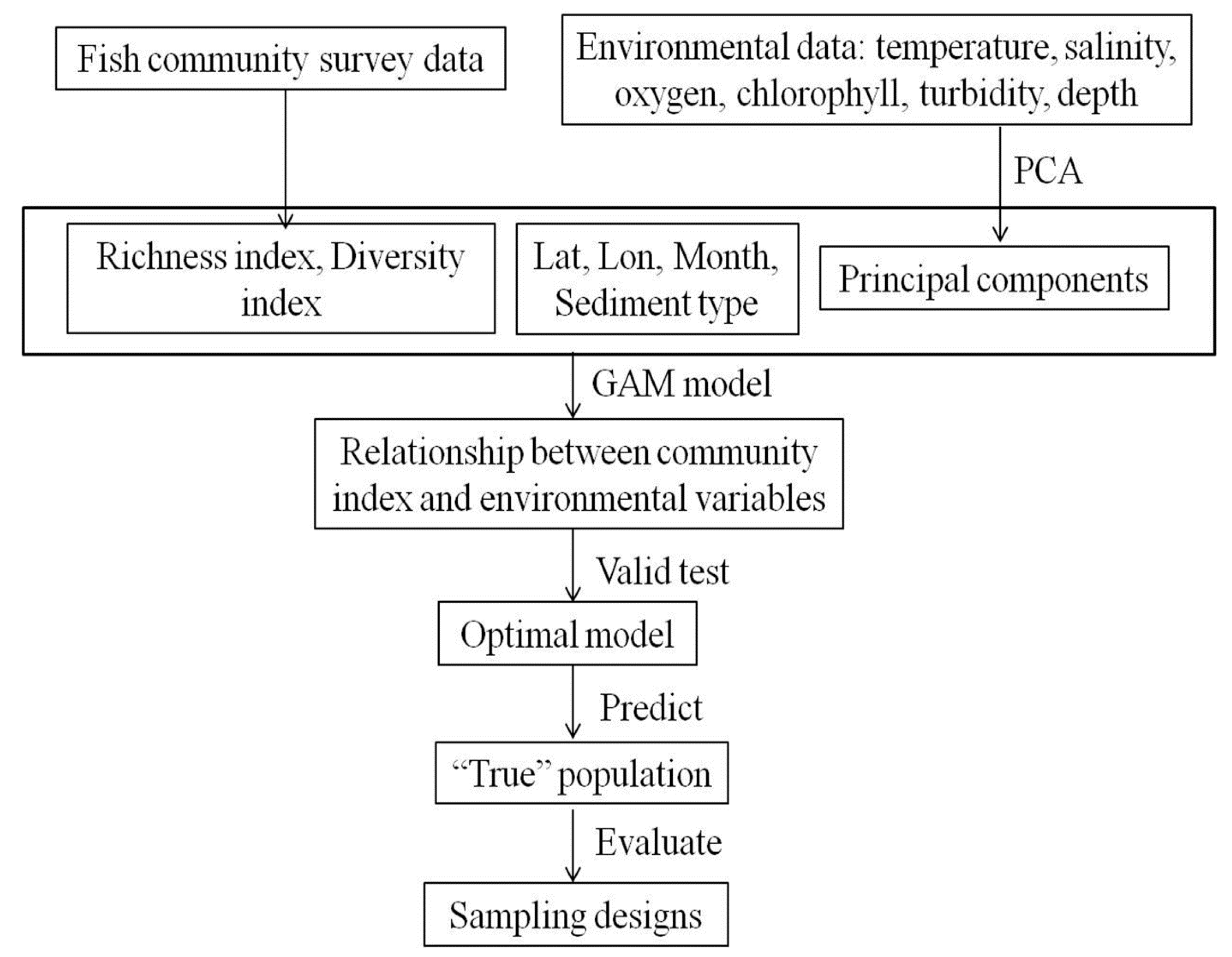
Figure 2.
The study area and sampling sites.

Figure 3.
Habitat type in study area and the distribution of demersal fish community index in October. (a) The distribution of Margalef’s richness index; and (b) The distribution of Shannon index.
Figure 3.
Habitat type in study area and the distribution of demersal fish community index in October. (a) The distribution of Margalef’s richness index; and (b) The distribution of Shannon index.


Figure 4.
The design effect (Deff) of different sampling designs for: (a) Margalef’s richness index, sample size was 25; (b) Shannon index, sample size was 25; (c) Margalef’s richness index, sample size was 50; (d) Shannon index, sample size was 50; (e) Margalef’s richness index, sample size was 100; and (f) Shannon index, sample size was 100.


Figure 5.
The relative estimation error (REE) of different sampling designs for (a) Margalef’s richness index, sample size was 25; (b) Shannon index, sample size was 25; (c) Margalef’s richness index, sample size was 50; (d) Shannon index, sample size was 50; (e) Margalef’s richness index, sample size was 100; and (f) Shannon index, sample was 100.


Figure 6.
Distribution of REE of different designs for: (a) Margalef’s richness index, sample size was 25; (b) Shannon index, sample size was 25; (c) Margalef’s richness index, sample size was 50; (d) Shannon index, sample size was 50; (e) Margalef’s richness index, sample size was 100; and (f) Shannon index, sample size was 100.


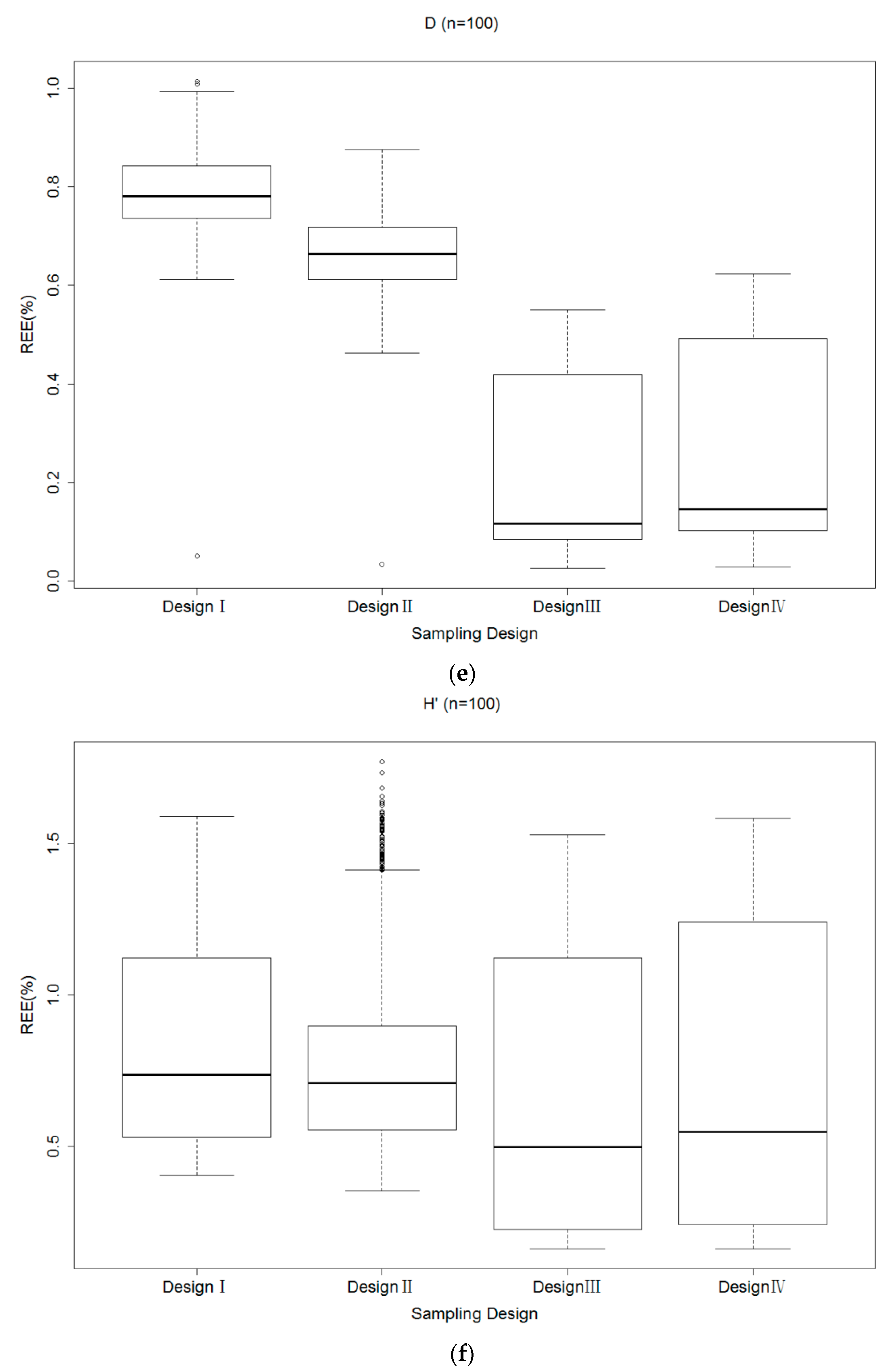
Figure 7.
Distribution of relative bias (RB) of different designs for (a) Margalef’s richness index, sample size was 25; (b) Shannon index, sample size was 25; (c) Margalef’s richness index, sample size was 50; (d) Shannon index, sample size was 50; (e) Margalef’s richness index, sample size was 100; and (f) Shannon index, sample was 100.


Figure 8.
Performance of Design III for the Margalef’s richness index with increased temperature for: (a) Deff; and (b) REE.
Figure 8.
Performance of Design III for the Margalef’s richness index with increased temperature for: (a) Deff; and (b) REE.


Table 1.
The Deff and REE for different sampling designs of Margalef’s richness index with a uniform temperature increase.
Table 1.
The Deff and REE for different sampling designs of Margalef’s richness index with a uniform temperature increase.
| Temperature Increase (°C) | Deff | REE (%) | |||||||
|---|---|---|---|---|---|---|---|---|---|
| I | II | III | IV | I | II | III | IV | ||
| 0 | Average | 1 | 0.580 | 0.002 | 0.003 | 1.180 | 0.920 | 0.053 | 0.063 |
| Coefficient of Variation (CV) | 0 | 0.240 | 0.100 | 0.190 | 0.290 | 0.380 | 0.320 | 0.370 | |
| 1 | Average | 1 | 0.600 | 0.002 | 0.003 | 1.110 | 0.890 | 0.054 | 0.064 |
| Coefficient of Variation (CV) | 0 | 0.200 | 0.070 | 0.050 | 0.350 | 0.430 | 0.320 | 0.350 | |
| 2 | Average | 1 | 0.610 | 0.002 | 0.003 | 1.108 | 0.880 | 0.053 | 0.064 |
| Coefficient of Variation (CV) | 0 | 0.200 | 0.090 | 0.020 | 0.340 | 0.430 | 0.320 | 0.360 | |
| 3 | Average | 1 | 0.600 | 0.0023 | 0.003 | 1.110 | 0.890 | 0.053 | 0.064 |
| Coefficient of Variation (CV) | 0 | 0.190 | 0.080 | 0.010 | 0.340 | 0.430 | 0.320 | 0.350 | |
| 4 | Average | 1 | 0.560 | 0.002 | 0.003 | 1.110 | 0.890 | 0.053 | 0.064 |
| Coefficient of Variation (CV) | 0 | 0.020 | 0.080 | 0.040 | 0.350 | 0.430 | 0.320 | 0.360 | |
| 5 | Average | 1 | 0.610 | 0.0024 | 0.003 | 1.110 | 0.880 | 0.053 | 0.064 |
| Coefficient of Variation (CV) | 0 | 0.180 | 0.060 | 0.030 | 0.340 | 0.430 | 0.320 | 0.350 | |
The smallest Deffand REE for each scenario are identified in the bold print.
Table 2.
The Deff and REE of each sampling design of Margalef’s richness index with a non-uniform temperature increase.
Table 2.
The Deff and REE of each sampling design of Margalef’s richness index with a non-uniform temperature increase.
| Temperature Scenario (°C) | Deff | REE (%) | |||||||
|---|---|---|---|---|---|---|---|---|---|
| I | II | III | IV | I | II | III | IV | ||
| 02–04 | Average | 1 | 0.730 | 0.002 | 0.002 | 1.230 | 1.050 | 1.140 | 1.140 |
| Cofficient of Variation (CV) | 0 | 0.290 | 0.240 | 0.200 | 0.280 | 0.330 | 0.004 | 0.004 | |
| 04–06 | Average | 1 | 0.730 | 0.011 | 0.015 | 1.240 | 1.041 | 1.180 | 1.180 |
| Cofficient of Variation (CV) | 0 | 0.290 | 0.270 | 0.200 | 0.300 | 0.340 | 0.013 | 0.015 | |
| 06–08 | Average | 1 | 0.680 | 0.160 | 0.190 | 1.290 | 1.060 | 1.300 | 1.310 |
| Cofficient of Variation (CV) | 0 | 0.290 | 0.270 | 0.200 | 0.300 | 0.350 | 0.070 | 0.067 | |
The smallest Deff and REE for each scenario are identified in the bold print. 02–04 means that the temperature for prediction came from April while keeping the other environmental variables invariant compared to February. 04–06 means that the temperature for prediction came from June while keeping the other environmental variables invariant compared to April. 06–08 means that the temperature for prediction came from August while keeping the other environmental variables invariant compared to June.
© 2018 by the authors. Licensee MDPI, Basel, Switzerland. This article is an open access article distributed under the terms and conditions of the Creative Commons Attribution (CC BY) license (http://creativecommons.org/licenses/by/4.0/).
Share and Cite
MDPI and ACS Style
Zhao, J.; Cao, J.; Tian, S.; Chen, Y.; Zhang, S. Evaluating Sampling Designs for Demersal Fish Communities. Sustainability 2018, 10, 2585. https://doi.org/10.3390/su10082585
AMA Style
Zhao J, Cao J, Tian S, Chen Y, Zhang S. Evaluating Sampling Designs for Demersal Fish Communities. Sustainability. 2018; 10(8):2585. https://doi.org/10.3390/su10082585
Chicago/Turabian StyleZhao, Jing, Jie Cao, Siquan Tian, Yong Chen, and Shouyu Zhang. 2018. "Evaluating Sampling Designs for Demersal Fish Communities" Sustainability 10, no. 8: 2585. https://doi.org/10.3390/su10082585
Note that from the first issue of 2016, this journal uses article numbers instead of page numbers. See further details here.