Analysis of Sustainability Decision Trees Generated by Qualitative Models Based on Equationless Heuristics

Abstract
:1. Introduction
- A dropped object falls straight down.
- A solid object cannot pass through another solid object.
- A vacuum sucks things towards it.
“if the ammoniac concentration is increasing, then its neutralisation cost is increasing.”
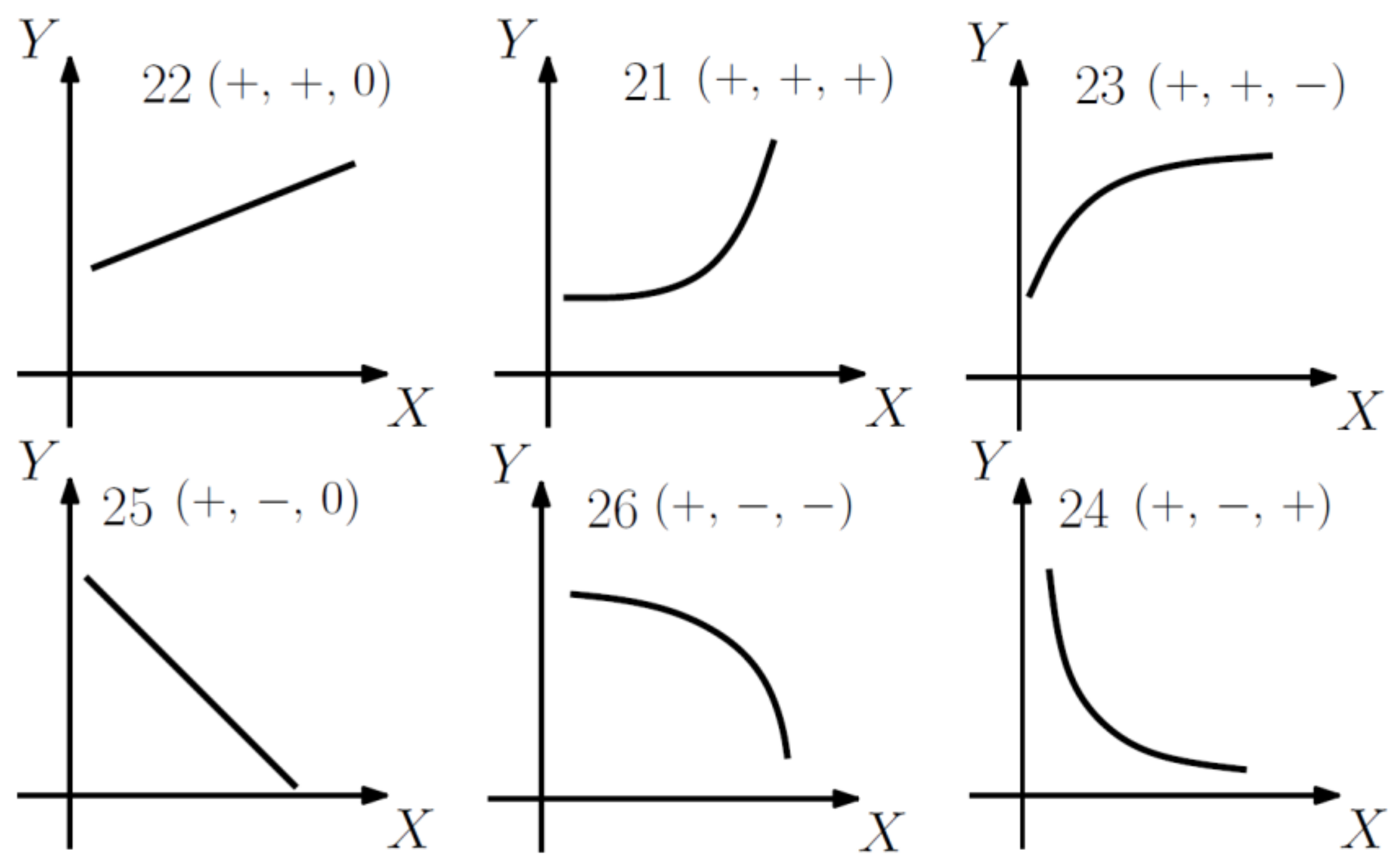
- The relation is increasing, the first derivative is therefore positive.
- The increase is more and more rapid, that is, the second derivative is therefore positive.
- If X = 0, then Y = positive.
2. Materials and Methods
2.1. Qualitative Models
- Contributing to a better understanding of the meaning of sustainability and its contextual interpretation (interpretation challenge);
- Integrating sustainability issues into decision-making by identifying and assessing (past and/or future) sustainability impacts (information-structuring challenge); and
- Fostering sustainability objectives (influence challenge).
If X1 is decreasing, then X2 is decreasing.
If X3 is increasing, then X2 is decreasing.
If X3 is decreasing, then X2 is increasing.
QP− X3 X2
QP− qualitative indirect proportionality.
1 22 (see Figure 1) X1 X2
2 26 (see Figure 1) X3 X2
| X1 | X2 | X3 | |
| 1 | + + + | + + + | + − − |
| 2 | + + 0 | + + + | + − − |
| 3 | + + − | + + + | + − − |
| 4 | + + − | + + 0 | + − − |
| 5 | + + − | + + − | + − + |
| 6 | + + − | + + − | + − 0 |
| 7 | + + − | + + − | + − − |
| 8 | + 0 + | + 0 + | + 0 − |
| 9 | + 0 0 | + 0 0 | + 0 0 |
| 10 | + 0 − | + 0 − | + 0 + |
| 11 | + − + | + − + | + + − |
| 12 | + − 0 | + − + | + + − |
| 13 | + − − | + − + | + + − |
| 14 | + − − | + − 0 | + + − |
| 15 | + − − | + − − | + + + |
| 16 | + − − | + − − | + + 0 |
| 17 | + − − | + − − | + + − |
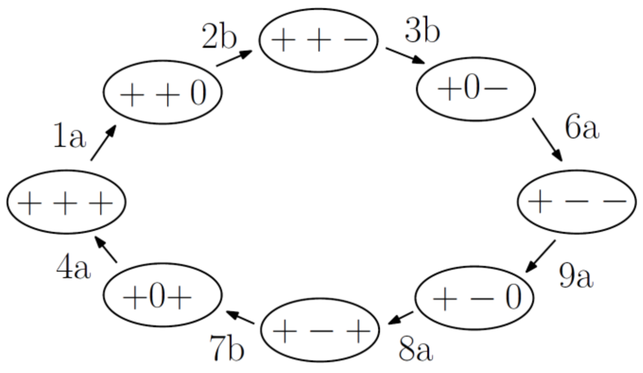
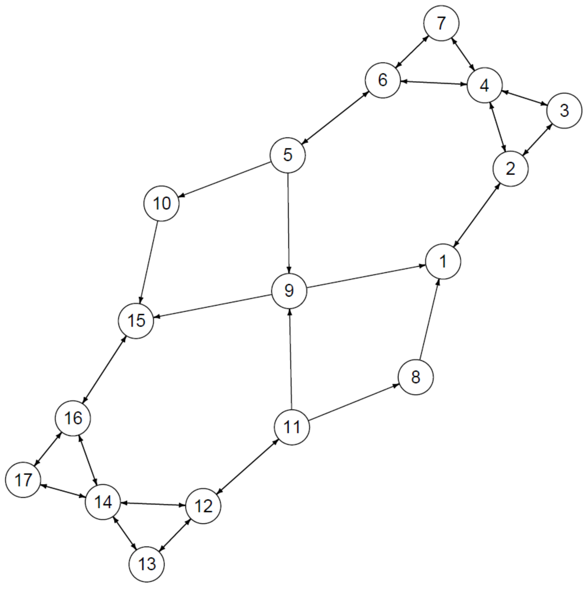
2.2. Transitional Graph
2.3. Sustainability Decision Making
2.4. Qualitative Trees Generated From Transition Graphs
2.5. Quantitative Evaluations of Qualitative Trees—Reconciliation
- Complete III, i.e., all of the numerical values needed to evaluate the decision tree using traditional algorithms are available;
- Total ignorance, not a single numerical value is available; and
- Partial ignorance, some numerical values are available.
3. Case Study
(see Model [7])
1 QP+ ROA VA
2 QP− CF CG
3 22 PL VA
4 QP− EAT TA
5 QP+ CG ERI
6 24 SPW PW
7 23 SPW CRE
8 24 SPW TA
9 21 CF ERI
10 QP− PL PW
11 24 ERI CRE
12 QP− SPW ERI
4. Results
5. Discussion
- Mathematical models, sets of differential and/or algebraic equations,
- ◦
- numerical/fuzzy, and so on, values of constants are not available.
- With numerical values of constants,
- ◦
- statistical models, for example, an exponential function such as the least squares algorithm.
- Experience,
- Analogy,
- Feelings.
6. Conclusions
Author Contributions
Funding
Acknowledgments
Conflicts of Interest
References
- Ness, B.; Urbel-Piirsalu, E.; Anderberg, S.; Olsson, L. Categorising tools for sustainability assessment. Ecol. Econ. 2007, 60, 498–508. [Google Scholar] [CrossRef]
- Bányai, T. Supply chain optimization of outsourced blending technologies. J. Appl. Econ. Sci. 2017, 12, 960–976. [Google Scholar]
- Bányai, T.; Veres, P.; Illés, B. Heuristic Supply Chain Optimization of Networked Maintenance Companies. Procedia Eng. 2015, 100, 46–55. [Google Scholar] [CrossRef]
- Li, Z.; Xu, Y.; Deng, F.; Liang, X. Impacts of Power Structure on Sustainable Supply Chain Management. Sustainability 2017, 10, 55. [Google Scholar] [CrossRef]
- Bommier, A.; Lanz, B.; Zuber, S. Models-as-usual for unusual risks? On the value of catastrophic climate change. J. Environ. Econ. Manag. 2015, 74, 1–22. [Google Scholar] [CrossRef]
- Allen, W.; Cruz, J.; Warburton, B. How Decision Support Systems Can Benefit from a Theory of Change Approach. Environ. Manag. 2017, 59, 956–965. [Google Scholar] [CrossRef] [PubMed]
- Day, B.; Pinto Prades, J.-L. Ordering anomalies in choice experiments. J. Environ. Econ. Manag. 2010, 59, 271–285. [Google Scholar] [CrossRef]
- Sen, P.K.; Singer, J.M. Large Sample Methods in Statistics: An Introduction with Applications; CRC Press: Boca Raton, FL, USA, 1994; ISBN 978-0-412-04221-8. [Google Scholar]
- Dohnal, M.; Kocmanová, A.; Rašková, H. Hi tech microeconomics and information nonintensive calculi. Trends Econ. Manag. 2013, 2, 20–26. [Google Scholar]
- Choueiry, B.Y.; Iwasaki, Y.; McIlraith, S. Towards a practical theory of reformulation for reasoning about physical systems. Artif. Intell. 2005, 162, 145–204. [Google Scholar] [CrossRef]
- Dohnal, M. A methodology for common-sense model development. Comput. Ind. 1991, 16, 141–158. [Google Scholar] [CrossRef]
- Dohnal, M. Naive models as active expert system in bioengineering and chemical engineering. Collect. Czechoslov. Chem. Commun. 1988, 53, 1476–1499. [Google Scholar] [CrossRef]
- Džeroski, S.; Grbović, J.; Walley, W.J.; Kompare, B. Using machine learning techniques in the construction of models. II. Data analysis with rule induction. Ecol. Model. 1997, 95, 95–111. [Google Scholar] [CrossRef]
- Klenk, M.; Forbus, K. Analogical model formulation for transfer learning in AP Physics. Artif. Intell. 2009, 173, 1615–1638. [Google Scholar] [CrossRef]
- Mueller, E.T. Commonsense Reasoning; Morgan Kaufmann: Burlington, MA, USA, 2010; ISBN 978-0-08-047661-2. [Google Scholar]
- Nayak, P.P. Causal Approximations. Artif. Intell. 1994, 70, 277–334. [Google Scholar] [CrossRef]
- Govindan, K.; Fattahi, M.; Keyvanshokooh, E. Supply chain network design under uncertainty: A comprehensive review and future research directions. Eur. J. Oper. Res. 2017, 263, 108–141. [Google Scholar] [CrossRef]
- Aalirezaei, A.; Aalirezaei, A. Designing Sustainable Recovery Network for Waste from Electrical and Electronic Equipment (WEEE) using Genetic Algorithm. Int. J. Environ. Sustain. Dev. 2016, 16, 60–79. [Google Scholar] [CrossRef]
- Dehghanian, F.; Mansour, S. Designing sustainable recovery network of end-of-life products using genetic algorithm. Resour. Conserv. Recycl. 2009, 53, 559–570. [Google Scholar] [CrossRef]
- Lipmann, O.; Bogen, H. Naive Physik Theoretische und Experimentelle Untersuchungen Über die Fähigkeit zu Intelligentem Handeln; Barth: Leipzig, Germany, 1923. [Google Scholar]
- De Kleer, J.; Brown, J.S. A qualitative physics based on confluences. Artif. Intell. 1984, 24, 7–83. [Google Scholar] [CrossRef]
- Dočekalová, M.P.; Kocmanová, A. Composite indicator for measuring corporate sustainability. Ecol. Indic. 2016, 61, 612–623. [Google Scholar] [CrossRef]
- Kocmanová, A.; Pavláková Dočekalová, M.; Škapa, S.; Smolíková, L. Measuring Corporate Sustainability and Environmental, Social, and Corporate Governance Value Added. Sustainability 2016, 8, 945. [Google Scholar] [CrossRef]
- Kratena, K.; Streicher, G. Spatial Welfare Economics versus Ecological Footprint: A Sensitivity Analysis Introducing Strong Sustainability. Environ. Resour. Econ. 2012, 51, 617–622. [Google Scholar] [CrossRef]
- Bond, C.A.; Farzin, Y.H. Alternative sustainability criteria, externalities, and welfare in a simple agroecosystem model: A numerical analysis. Environ. Resour. Econ. 2008, 40, 383–399. [Google Scholar] [CrossRef]
- Seghezzo, L.; Venencia, C.; Catalina Buliubasich, E.; Iribarnegaray, M.A.; Volante, J.N. Participatory, Multi-Criteria Evaluation Methods as a Means to Increase the Legitimacy and Sustainability of Land Use Planning Processes. The Case of the Chaco Region in Salta, Argentina. Environ. Manag. 2017, 59, 307–324. [Google Scholar] [CrossRef] [PubMed]
- Banerjee, A.; Halvorsen, K.E.; Eastmond-Spencer, A.; Sweitz, S.R. Sustainable Development for Whom and How? Exploring the Gaps between Popular Discourses and Ground Reality Using the Mexican Jatropha Biodiesel Case. Environ. Manag. 2017, 59, 912–923. [Google Scholar] [CrossRef] [PubMed]
- Bredeweg, B.; Linnebank, F.; Bouwer, A.; Liem, J. Garp3—Workbench for qualitative modelling and simulation. Ecol. Inform. 2009, 4, 263–281. [Google Scholar] [CrossRef]
- Vicha, T.; Dohnal, M. Qualitative identification of chaotic systems behaviours. Chaos Solitons Fractals 2008, 38, 70–78. [Google Scholar] [CrossRef]
- Forbus, K.D. Qualitative reasoning. In CRC Handbook of Computer Science and Engineering; CRC Press: Boca Raton, FL, USA, 1996. [Google Scholar]
- Dohnal, M. Complex biofuels related scenarios generated by qualitative reasoning under severe information shortages: A review. Renew. Sustain. Energy Rev. 2016, 65, 676–684. [Google Scholar] [CrossRef]
- Waas, T.; Hugé, J.; Block, T.; Wright, T.; Benitez-Capistros, F.; Verbruggen, A. Sustainability Assessment and Indicators: Tools in a Decision-Making Strategy for Sustainable Development. Sustainability 2014, 6, 5512–5534. [Google Scholar] [CrossRef] [Green Version]
- Faucheux, S.; Froger, G. Decision-making under environmental uncertainty. Ecol. Econ. 1995, 15, 29–42. [Google Scholar] [CrossRef]
- Lee, S.; Lee, C.-W. Application of Decision-Tree Model to Groundwater Productivity-Potential Mapping. Sustainability 2015, 7, 13416–13432. [Google Scholar] [CrossRef] [Green Version]
- Mikučionienė, R.; Martinaitis, V.; Keras, E. Evaluation of energy efficiency measures sustainability by decision tree method. Energy Build. 2014, 76, 64–71. [Google Scholar] [CrossRef]
- Garcia-Garcia, G.; Woolley, E.; Rahimifard, S.; Colwill, J.; White, R.; Needham, L. A Methodology for Sustainable Management of Food Waste. Waste Biomass Valor 2017, 8, 2209–2227. [Google Scholar] [CrossRef] [Green Version]
- Munda, G. Multiple criteria decision analysis and sustainable development. In Multiple Criteria Decision Analysis: State of the Art Surveys; International Series in Operations Research & Management Science; Springer: New York, NY, USA, 2005; pp. 953–986. ISBN 978-0-387-23067-2. [Google Scholar]
- Rose, L.M. Engineering Investment Decisions: Planning Under Uncertainty; Elsevier Science Ltd.: Amsterdam, The Netherlands, 1976; ISBN 978-0-444-41522-6. [Google Scholar]
- Burfurd, I.; Gangadharan, L.; Nemes, V. Stars and standards: Energy efficiency in rental markets. J. Environ. Econ. Manag. 2012, 64, 153–168. [Google Scholar] [CrossRef]
- Phadatare, M.M.; Nandgaonkar, S.S. Uncertain data mining using decision tree and bagging technique. Int. J. Comput. Sci. Inf. Technol. 2014, 5, 3069–3073. [Google Scholar]
- Butler, A.W.; Keefe, M.O.; Kieschnick, R. Robust determinants of IPO underpricing and their implications for IPO research. J. Corp. Financ. 2014, 27, 367–383. [Google Scholar] [CrossRef]
- Zhu, H.; Zhang, C.; Li, H.; Chen, S. Information environment, market-wide sentiment and IPO initial returns: Evidence from analyst forecasts before listing. China J. Account. Res. 2015, 8, 193–211. [Google Scholar] [CrossRef]
- Danielson, M.; Ekenberg, L.; Larsson, A. Distribution of expected utility in decision trees. Int. J. Approx. Reason. 2007, 46, 387–407. [Google Scholar] [CrossRef]
- Nie, G.; Zhang, L.; Liu, Y.; Zheng, X.; Shi, Y. Decision analysis of data mining project based on Bayesian risk. Expert Syst. Appl. 2009, 36, 4589–4594. [Google Scholar] [CrossRef]
- Doubravsky, K.; Dohnal, M. Reconciliation of Decision-Making Heuristics Based on Decision Trees Topologies and Incomplete Fuzzy Probabilities Sets. PLoS ONE 2015, 10, e0131590. [Google Scholar] [CrossRef] [PubMed]
- Dohnal, M.; Vykydal, J.; Kvapilik, M.; Bures, P. Practical uncertainty assessment of reasoning paths (fault trees) under total uncertainty ignorance. J. Loss Prev. Process Ind. 1992, 5, 125–131. [Google Scholar] [CrossRef]
- Klüppelberg, C.; Straub, D.; Welpe, I.M. (Eds.) Risk—A Multidisciplinary Introduction; Springer: Cham, Switzerland, 2014; ISBN 978-3-319-04485-9. [Google Scholar]
- Dohnal, M. Ignorance and uncertainty in reliability reasoning. Microelectron. Reliab. 1992, 32, 1157–1170. [Google Scholar] [CrossRef]
- Watson, S.R. The meaning of probability in probabilistic safety analysis. Reliab. Eng. Syst. Saf. 1994, 45, 261–269. [Google Scholar] [CrossRef]
- Behera, D.; Chakraverty, S. Solving fuzzy complex system of linear equations. Inf. Sci. 2014, 277, 154–162. [Google Scholar] [CrossRef]
- Huang, C.-F.; Tsai, M.-Y.; Hsieh, T.-N.; Kuo, L.-M.; Chang, B.R. A study of hybrid genetic-fuzzy models for IPO stock selection. In Proceedings of the International Conference on Fuzzy Theory and it’s Applications (iFUZZY), Taichung, Taiwan, 16–18 November 2012; pp. 357–362. [Google Scholar]


| Values: | Positive | Zero | Negative | Anything |
|---|---|---|---|---|
| Derivatives: | Increasing | Constant | Decreasing | Any direction |
| Symbol: | + | 0 | – | * |
| From | To | Or | Or | Or | Or | Or | Or | ||
|---|---|---|---|---|---|---|---|---|---|
| a | b | c | d | e | f | g | |||
| 1 | + + + | → | + + 0 | ||||||
| 2 | + + 0 | → | + + + | + + − | |||||
| 3 | + + − | → | + + 0 | + 0 − | + 0 0 | ||||
| 4 | + 0 + | → | + + + | ||||||
| 5 | + 0 0 | → | + + + | + − − | |||||
| 6 | + 0 − | → | + − − | ||||||
| 7 | + − + | → | + − 0 | + 0 + | + 0 0 | 0 − + | 0 0 + | 0 0 0 | 0 − 0 |
| 8 | + − 0 | → | + − + | + − − | 0 − 0 | ||||
| 9 | + − − | → | + − 0 | 0 − − | 0 − 0 | ||||
| 10 | 0 + + | → | + + 0 | + + − | + + + | ||||
| 11 | 0 + 0 | → | + + 0 | + + − | + + + | ||||
| 12 | 0 + − | → | + + − | ||||||
| 13 | 0 0 + | → | + + + | ||||||
| 14 | 0 0 0 | → | + + + | − − − | |||||
| 15 | 0 0 − | → | − − − | ||||||
| 16 | 0 − + | → | − − + | ||||||
| 17 | 0 − 0 | → | − − 0 | − − + | − − − | ||||
| 18 | 0 − − | → | − − 0 | − − + | − − − | ||||
| 19 | − + + | → | − + 0 | 0 + + | 0 + 0 | ||||
| 20 | − + 0 | → | − + − | − + + | 0 + 0 | ||||
| 21 | − + − | → | − + 0 | − 0 − | − 0 0 | 0 + − | 0 0 − | 0 0 0 | 0 + 0 |
| 22 | − 0 + | → | − + + | ||||||
| 23 | − 0 0 | → | − + + | − − − | |||||
| 24 | − 0 − | → | − − − | ||||||
| 25 | − − + | → | − − 0 | − 0 + | − 0 0 | ||||
| 26 | − − 0 | → | − − − | − − + | |||||
| 27 | − − − | → | − − 0 |
| X1 | X2 | Θ | |
|---|---|---|---|
| 1 | + + + | + + + | + − − |
| 2 | + 0 − | + − − | + + + |
| 3 | + − − | + − + | + − + |
| Variable | Label |
|---|---|
| Cash Flow | CF |
| Return on Assets | ROA |
| Value Added | VA |
| Earnings after taxes | EAT |
| Ecology related investments | ERI |
| Consumption of renewable energy | CRE |
| Production of waste | PW |
| Productivity of labour | PL |
| Corporate governance | CG |
| Variable | Label |
|---|---|
| Sustainability Political Will | SPW |
| Taxes | TA |
| PL | VA | ROA | CRE | CF | PW | EAT | TA | CG | SPW | ERI | |
|---|---|---|---|---|---|---|---|---|---|---|---|
| 1 | + + * | + + * | + + * | + + * | + − * | + − * | + + * | + − * | + − * | + + * | + − * |
| 2 | + 0 * | + 0 * | + 0 * | + 0 * | + 0 * | + 0 * | + 0 * | + 0 * | + 0 * | + 0 * | + 0 * |
| 3 | + − * | + − * | + − * | + − * | + + * | + + * | + − * | + + * | + + * | + − * | + + * |
| PL | VA | ROA | CRE | CF | PW | EAT | TA | CG | SPW | ERI |
|---|---|---|---|---|---|---|---|---|---|---|
| ↑ | ↑ | ↑ | ↑ | ↑ | ↓ | ↑ | ↓ | ↑ | ↑ | ↑ |
| PL | VA | ROA | CRE | CF | PW | EAT | TA | CG | SPW | ERI | |
|---|---|---|---|---|---|---|---|---|---|---|---|
| 1 | + + + | + + + | + + + | + + + | + − − | + − − | + + + | + − − | + − − | + + + | + − − |
| 2 | + + + | + + + | + + + | + + + | + − − | + − − | + + 0 | + − 0 | + − − | + + + | + − − |
| 3 | + + + | + + + | + + + | + + + | + − − | + − − | + + − | + − + | + − − | + + + | + − − |
| 4 | + + 0 | + + 0 | + + 0 | + + + | + − − | + − 0 | + + + | + − − | + − − | + + + | + − − |
| 5 | + + 0 | + + 0 | + + 0 | + + + | + − − | + − 0 | + + 0 | + − 0 | + − − | + + + | + − − |
| 6 | + + 0 | + + 0 | + + 0 | + + + | + − − | + − 0 | + + − | + − + | + − − | + + + | + − − |
| 7 | + + − | + + − | + + − | + + + | + − − | + − + | + + + | + − − | + − − | + + + | + − − |
| 8 | + + − | + + − | + + − | + + + | + − − | + − + | + + 0 | + − 0 | + − − | + + + | + − − |
| 9 | + + − | + + − | + + − | + + + | + − − | + − + | + + − | + − + | + − − | + + + | + − − |
| 10 | + + − | + + − | + + − | + + − | + − + | + − + | + + − | + − + | + − + | + + − | + − + |
| 11 | + + − | + + − | + + − | + + − | + − 0 | + − + | + + − | + − + | + − + | + + − | + − + |
| 12 | + + − | + + − | + + − | + + − | + − − | + − + | + + − | + − + | + − + | + + − | + − + |
| 13 | + 0 + | + 0 + | + 0 + | + 0 + | + 0 − | + 0 − | + 0 + | + 0 − | + 0 − | + 0 + | + 0 − |
| 14 | + 0 0 | + 0 0 | + 0 0 | + 0 0 | + 0 0 | + 0 0 | + 0 0 | + 0 0 | + 0 0 | + 0 0 | + 0 0 |
| 15 | + 0 − | + 0 − | + 0 − | + 0 − | + 0 + | + 0 + | + 0 − | + 0 + | + 0 + | + 0 − | + 0 + |
| 16 | + − + | + − + | + − + | + − + | + + − | + + − | + − + | + + − | + + − | + − + | + + − |
| 17 | + − + | + − + | + − + | + − + | + + − | + + − | + − 0 | + + 0 | + + − | + − + | + + − |
| 18 | + − + | + − + | + − + | + − + | + + − | + + − | + − − | + + + | + + − | + − + | + + − |
| 19 | + − 0 | + − 0 | + − 0 | + − + | + + − | + + 0 | + − + | + + − | + + − | + − + | + + − |
| 20 | + − 0 | + − 0 | + − 0 | + − + | + + − | + + 0 | + − 0 | + + 0 | + + − | + − + | + + − |
| 21 | + − 0 | + − 0 | + − 0 | + − + | + + − | + + 0 | + − − | + + + | + + − | + − + | + + − |
| 22 | + − − | + − − | + − − | + − + | + + − | + + + | + − + | + + − | + + − | + − + | + + − |
| 23 | + − − | + − − | + − − | + − + | + + − | + + + | + − 0 | + + 0 | + + − | + − + | + + − |
| 24 | + − − | + − − | + − − | + − + | + + − | + + + | + − − | + + + | + + − | + − + | + + − |
| 25 | + − − | + − − | + − − | + − − | + + + | + + + | + − − | + + + | + + + | + − − | + + + |
| 26 | + − − | + − − | + − − | + − − | + + 0 | + + + | + − − | + + + | + + + | + − − | + + + |
| 27 | + − − | + − − | + − − | + − − | + + − | + + + | + − − | + + + | + + + | + − − | + + + |
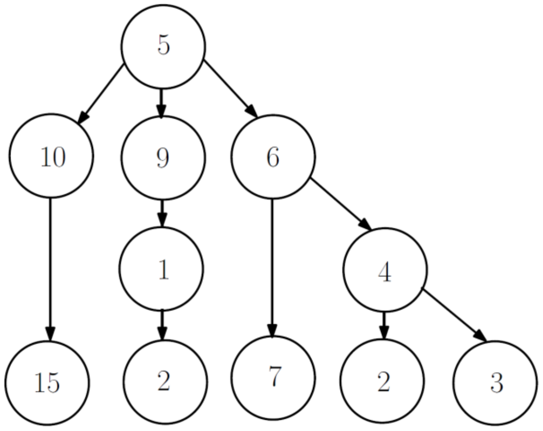
| Scenario i (See Figure 7) | Utility ui |
|---|---|
| 3 | 0.727 |
| 6 | 0.727 |
| 7 | 0.727 |
| 9 | 0.727 |
| 27 | 0.272 |
| Transition from i to j | Fuzzy Probability | |||
|---|---|---|---|---|
| i | j | a | b = c | d |
| 1 | 5 | 0.5 | 0.6 | 0.65 |
| 1 | 4 | 0.25 | 0.3 | 0.4 |
| 14 | 25 | 0.6 | 0.7 | 0.8 |
| 14 | 1 | 0.35 | 0.4 | 0.45 |
| Transition from Scenario i to Scenario j (See Figure 7) | Probability of Transition | |
|---|---|---|
| i | j | P |
| 14 | 25 | 0.6 |
| 14 | 1 | 0.4 |
| 25 | 26 | 1 |
| 26 | 27 | 1 |
| 1 | 4 | 0.3 |
| 1 | 5 | 0.5 |
| 1 | 2 | 0.2 |
| 4 | 7 | 0.667 |
| 4 | 8 | 0.333 |
| 5 | 9 | 1 |
| 2 | 3 | 1 |
| 8 | 6 | 1 |
| Terminal | Utility | Probability | ui·Pi |
|---|---|---|---|
| i | ui | Pi | |
| 3 | 0.727 | 0.08 | 0.058 |
| 6 | 0.727 | 0.04 | 0.029 |
| 7 | 0.727 | 0.08 | 0.058 |
| 9 | 0.727 | 0.2 | 0.145 |
| 27 | 0.272 | 0.6 | 0.163 |
© 2018 by the authors. Licensee MDPI, Basel, Switzerland. This article is an open access article distributed under the terms and conditions of the Creative Commons Attribution (CC BY) license (http://creativecommons.org/licenses/by/4.0/).
Share and Cite
Doubravský, K.; Kocmanová, A.; Dohnal, M. Analysis of Sustainability Decision Trees Generated by Qualitative Models Based on Equationless Heuristics. Sustainability 2018, 10, 2505. https://doi.org/10.3390/su10072505
Doubravský K, Kocmanová A, Dohnal M. Analysis of Sustainability Decision Trees Generated by Qualitative Models Based on Equationless Heuristics. Sustainability. 2018; 10(7):2505. https://doi.org/10.3390/su10072505
Chicago/Turabian StyleDoubravský, Karel, Alena Kocmanová, and Mirko Dohnal. 2018. "Analysis of Sustainability Decision Trees Generated by Qualitative Models Based on Equationless Heuristics" Sustainability 10, no. 7: 2505. https://doi.org/10.3390/su10072505
APA StyleDoubravský, K., Kocmanová, A., & Dohnal, M. (2018). Analysis of Sustainability Decision Trees Generated by Qualitative Models Based on Equationless Heuristics. Sustainability, 10(7), 2505. https://doi.org/10.3390/su10072505