Greenhouse Gas Emissions from Intra-National Freight Transport: Measurement and Scenarios for Greater Sustainability in Spain

Abstract

Greenhouse Gas (GHG) emissions is a topic of major concern worldwide. Following previous articles which provide a methodology for estimating GHG emissions associated with international trade by transport mode at the world level, in this paper, we estimate an equivalent database of GHG emissions for inter-regional trade flows within a country (Spain). To this end, we built a new database of GHG emissions for origin–destination flows between Spanish provinces during 1995–2015. For each year, we combine industry-specific flows by four transport modes (road, train, ship and aircraft) with the corresponding GHG emissions factor for each mode in tons*km, drawn from the specialized literature. With this dataset of GHG emissions, we generate and analyze the temporal, sectoral and spatial pattern of Spanish inter-regional GHG flows. We then forecast emissions for 2016–2030 and consider how transport mode shifts might produce a more sustainable freight system within the country through the substitution of environmentally friendly alternatives (railway) for specific origin–destination–product flows in high-polluting modes (road).

1. Introduction

In December 2015, at the Paris climate conference (COP21), 195 countries adopted the first universal, legally binding global climate deal, with the aim of keeping global warming below 2 °C. All signatories were to turn their commitments into concrete policy actions after COP21 and report periodically on their progress. The European Union (EU) was the first major economy to submit its intended contribution to the new agreement in March 2015, pledging an ambitious 40% reduction of greenhouse gas emissions by 2030 from 1990 levels [1,2]. This target was in line with the EU’s previous “2030 climate and energy framework” [3] and with the European Commission’s “White Paper of Transport” from 2011 [4].

The EU’s 40% reduction of GHG emissions by 2030 has two parts: On the one hand, sectors covered by the emissions trading system (ETS) will have to lower emissions by 43% from 2005 levels. Sectors outside the ETS, which include the “transport sector”, will need to reduce them by 30% from 2005 levels. For these sectors, the Effort Sharing Decision (ESD) sets the maximum annual tonnage of GHG emissions for each EU member state based on its relative wealth (GDP per capita).

As suggested in several official documents [2,4,5], transport generates about a quarter of EU GHG emissions and is the second-most-polluting sector, after energy. However, while other sectors have seen their GHG emissions decrease, transport has seen them rise. Moreover, the transport modes with the sharpest increase in traffic have also had the largest increase in GHG emissions. From 1990 to 2012, international aviation, international shipping and road transport saw increases of 93%, 32% and 17%, respectively.

The EC’s 2011 “White Paper of Transport” [4] put forward several non-binding longer-term targets for the transport sector, with an overall goal to cut transport GHG emissions by at least 60% by 2050 (with respect to 1990 levels). Some reductions have been achieved since 2008, and transport GHG emissions fell by 3.3% in 2012, with the biggest reduction in road (3.6%) and aviation (1.3%). However, in 2012, EU transport emissions remained 20.5% above 1990 levels and will need to fall 67% by 2050.

According to a recent report [5], heavy duty vehicles (HDVs) were responsible for around 30% of road transport emissions, that is, more than 5% of EU GHG emissions and around 10% of total non-ETS emissions. This implies that less than 5% of all vehicles on the road emit around 30% of road transport CO₂ emissions. Moreover, forecasts for this highly polluting mode are negative: HDV emissions are projected to rise 22% by 2030.

In light of these trends, the EC has adopted a new strategy to promote low-emissions mobility, for both passengers and freight [2], proposing several measures to curtail excessive use of the road mode. In parallel, all member states, including Spain, are increasing their efforts to meet the general commitment and hit each specific target. In all cases, accurate measurements of and follow-up on emissions are critical.

As Davydenko et al. suggested [6], if we are to see gains in transport efficiency, we will need to establish a certain basis of comparison between the different methods of calculating emissions. This basis should be set at both the national and the international level, and cover the full extent of the complex logistical chain, door to door. As these authors reported, there is to date “no single globally-recognized and accepted standard for the calculation of the carbon footprint that covers the entire freight transport supply chain”. They used as their benchmark the EN-16258 methodology for the calculation of transport-service GHG emissions and laid out the criteria for an accurate methodology. Note that, in 2012, the European Committee for Standardisation (CEN) published European norm EN 16258 “Methodology for calculation and declaration of energy consumption and GHG emissions of transport services (freight and passengers)” (CEN standard EN 16258), which is the only official international—though European—standard aiming at the specific topic of transport supply chains. Davydenko et al. [6], also set forth three levels of aggregation at which transport-sector GHG emissions can be obtained: “micro”, “meso” and “macro”.

Keeping Davydenko et al. [6] and their categories in mind, we now turn to the Spanish case. At the “macro” level, the main official effort to compute GHG emissions is the Informative Inventory Report (IIR), produced by the Spanish National Inventory System (SEI) within the Ministry of Agriculture and Fishing, Food and Environment [7]. The 2018 IIR report was compiled in the context of the United Nations Economic Commission for Europe (UNECE) Convention on Long-Range Transboundary Air Pollution (CLRTAP), and contains detailed information on annual emissions estimates of air quality pollutants by source in Spain for the EMEP domain (excluding the Canary Islands) from 1990 onwards. According to the last IIR report, the “energy sector” generates more than 50% of the Inventory’s emitted pollutants. Within the “energy sector”, transport accounts for a large share of current emissions, with road transport being the worst offender. This subcategory encompasses pollutant emissions from vehicular traffic, including both passengers and freight.

The IIR’s methodology is thorough, involving the use of hundreds of variables at the production and consumption levels. Transport emissions are estimated through a detailed process, mainly based on the national figures for energy use by transport mode. Although the number of statistics is large, the estimation essentially follows a top-down approach, where the specific origin–destination–product–mode for each flow is given scant attention. Moreover, the Spanish IIR does not offer a sub-national allocation of GHG emissions by sector, but just a raw top-down aggregate imputation with no detail for the “transport sector”. Exact allocation of responsibility for polluting activities within the country is thus not possible [8]. This becomes critical when we consider sub-national entities within a highly decentralized country such as Spain, where not just the national government but also the regions (Nuts 2), provinces (Nuts 3) and municipalities (Nuts 5) are co-responsible for moderating GHG emissions. To this regard, it is interesting to consider, for example, how regions and cities are responsible for the development and control of transport infrastructures and services within urban areas, that is, the areas of densest congestion and pollution. Similarly, in Spain, Municipalities, Diputaciones Provinciales and Comunidades Autónomas all share with the national government various responsibilities with respect to follow-up on the quality of fresh water for human consumption. Similar arrangements exist for the management of waste, residuals, etc. Both COP21 and the “European Strategy for Low-Emission Mobility” [1,2] make a point of recognizing the role that sub-national entities (cities and regions) must play in any policy aiming to foster a more sustainable economy.

As Cristae et al. [9] noted, the situation within Spain is similar to the one observed for the international freight flows worldwide. While the International Transportation Forum uses a top-down approach to generate aggregate estimates of emissions from international transport, Cristea et al. suggested an alternative bottom-up procedure that more clearly allocates responsibility for pollution across countries and sectors. In fact, they highlighted the convenience of bottom-up approaches, where data on GHG emissions by mode are combined with data on traffic (tons*km) by mode, and detailed information is provided on the origin–destination and product type for each delivery.

In line with the methodology of Cristea et al. [9] for international freight flows and the recommendations of Davydenko et al. [6] for GHG estimation at the shipment level, this paper aims to estimate GHG emissions for intra- and inter-provincial freight flows within a country (Spain). GHG emissions for freight flows within a country are commonly estimated with input–output frameworks and CGE modeling [1,7,10,11,12]. However, with the exception of inter-regional input–output tables [13,14], it is impossible using this method to allocate emissions by specific origin–destination–product flows. The main reason, as Cristea et al. pointed out [9], is scarcity of data on origin–destination flows at the sectoral level in most countries. To the best of our knowledge, there has been no previous attempt with our methodology to cover origin–destination emissions for freight flows in Spain or any other EU country.

Drawing from a previous investigation [15], which develops and applies a detailed inter-provincial trade dataset to analyze transport-mode competition within Spain for a given year (2007), we build an extended database on intra- and inter-provincial freight flows and use it to obtain GHG emissions for origin–destination flows between Spanish provinces during 1995–2015. Note that, by adopting the province (Nuts 3) as the spatial unit of reference, we approached as close as possible to city-level figures, since for most Spanish provinces the capital city agglomerates the bulk of the population and economic activity. The flow data are based on a permanent dataset that was collected and prepared by the C-intereg Project (www.c-intereg.es) and based on the country’s most detailed available data on origin–destination–product statistics for freight flows by transport mode (road, train, ship and aircraft). The C-intereg project generates alternative figures covering intra-national Spanish trade at different spatial and sectoral levels. The data available to the public on the website are censored to some degree, while the sponsoring institutions and the research group in CEPREDE have access to the full detailed data. We used the full detailed data, especially “raw freight flows” measured in tons. By raw we mean closest to official figures on freight flows reported independently by the institution responsible for each mode in Spain (e.g., Ministerio de Fomento for road, RENFE for railway, Puertos del Estado for ship, and AENA for aircraft). We use this dataset to forecast the origin–destination–product–mode flows for 2015–2030 by means of gravity models, using intra- and inter-provincial origin–destination distance by mode, as well as the predictions described before about the evolution of provincial GDP in Spain for the same period.

In addition, for each transport mode and year, we build a corresponding dataset for GHG emissions, measured in gCO₂ per tons*km. These indicators cover 1995–2015 and are drawn from estimates already published by official institutions and other sound academic publications in the field. We then generate forecasts for 2015–2030 for each mode, extrapolating observed time trends.

Next, in line with the EN-16258 methodology [6], for each year, we combined industry-specific flows for each of the four transport modes, measured in tons*km, with the corresponding GHG emissions factors. Once the dataset of GHG emissions is built, we generate and analyze the temporal, sectoral and spatial patterns of Spanish inter-provincial GHG flows, and compare them with official national figures. Then, to search for a more sustainable freight system within the country, we address the possibility of promoting transport mode shifts from high-polluting modes (road) to more environmentally friendly alternatives (railway) for specific origin–destination–product flows. Two scenarios for transport mode shifts are considered, both inspired by targets suggested by the EC’s “White Paper of Transport” [4] and striving to achieve railway’s desirable future share.

To return to the conceptual framework suggested by Davydenko et al. [6], the methodology developed herein does not fulfil all of the authors’ recommendations. It fits in with their “meso” level and should be considered complementary to the “macro” official estimates published by the Spanish IIR. It includes at least two relevant aspects explicitly considered by the authors: the estimation of emissions at the shipment level, with the origin–destination–product–mode for each delivery; and the use of actual freight flows in volume and actual distance traveled by each mode for each origin–destination delivery. Because of data constraints, the main limitations of our methodology by comparison with the holistic approach described by Davydenko et al. [6] are: (i) lack of information on multimodal deliveries (our methodology assumes that points of origin and destination for each delivery correspond to points of production and consumption and does not consider multimodality); (ii) lack of information on GHG emissions associated with product handling at the origin and destination or with intermodal-connections; (iii) lack of information on the vehicle type used in each delivery; and (iv) lack of information on specific routes taken by freight haulers on their deliveries.

The rest of the paper is structured as follows: Section 2 reviews recent literature on the measurement and reduction of GHG emissions for freight flows at the international, European and country level, with a final focus on Spain. Section 3 describes our empirical estimation strategy for GHG emissions within Spain. Subsections lay out our two parallel datasets (origin–destination freight flows vs. GHG emissions indicators) and the two periods considered (1995–2015 vs. 2016–2030). Section 4 is an empirical analysis of trade and emissions patterns for each region, product type and transportation mode, and concludes with a description of the main results for the suggested scenarios.

2. GHG Emissions and Freight Flows

In the Introduction, we cite Davydenko et al. [6], who stressed the need for a standard measurement of the transport sector’s GHG emissions. However, there have been other approaches to the topic for given countries and other attempts to deal with the usual data constraints. An interesting paper in this regard was presented by McKinnon and Piecyk [16], and reviews several ways to estimate CO₂ emissions from freight transport flows. They claimed that, despite the interest of alternative estimation methods, the variability in the figures from official sources to academic approaches can erode the confidence of industry stakeholders in the validity of the estimates. McKinnon and Piecyk [16] used UK data, focused on the road mode, and evaluated various estimation methods for national emissions in a given year. More specifically, they considered four alternative methodologies used in the UK in 2006. Two are taken directly from official government sources, while the others are calculated by the authors: (i) National Environmental Accounts estimate for the “road transport of freight”; (ii) HGV-activity of British-registered haulers on UK roads using survey-based fuel efficiency estimates; (iii) all HGV-activity using survey-based fuel efficiency estimates; and (iv) all HGV-activity in the UK using test-cycle fuel efficiency estimates. These four approaches differ mainly in the scope of their calculations, their methodology and their alignment of vehicle classifications. The two lowest estimates relate solely to British-registered operators and therefore provide only a partial view of road freight activity in the UK. As this reference illustrates, an academic estimate such as ours can differ from the alternative official one, if only because of the use of alternative road data. McKinnon and Piecyk [16] based their calculations on heavy truck surveys or on traffic stations. One limitation of their approach is the lack of detail at the delivery level, which makes it difficult to assign responsibility for emissions at the sub-national level.

As noted in the Introduction, another interesting reference among the short literature analyzing GHG emissions associated with international trade using origin–destination flows by mode was presented by Cristae et al. [9], who collected extensive data on worldwide trade by transport mode and used it to provide detailed comparisons of GHG emissions associated with output versus international transport of traded goods. According to their analysis, international transport is responsible for 33% of worldwide trade-related emissions and over 75% of emissions for major manufacturing categories. Their approach covers emissions associated with both the production (output) and the transport of goods to destinations abroad, and allows them to distinguish between the two. Moreover, for the latter, they also considered the scale effect (i.e., changes in emissions due to changes in demand for international transport) and the composition effect (i.e., changes in the mode mix). They concluded that including transport dramatically changes the ranking of countries by emissions per dollar of trade. They also investigated whether trade inclusive of transport can lower emissions. In one quarter of cases, the difference in output emissions is more than enough to compensate for the emissions cost of transport. More interestingly for us, they also tested how likely patterns of global trade growth could affect modal use and emissions. According to their results, full liberalization of tariffs and GDP growth concentrated in China and India should lead to much faster growth in transport emissions than in the value of trade, because of shifts toward distant trading partners. However, the main limitation of their approach is to consider international trade in isolation from internal freight flows, which in most countries [17,18] account for a larger share of economic activity.

Whereas McKinnon and Piecyk [16] covered the entire UK, Zanni and Bristow [19] analyzed CO₂ emissions for freight flows in London, using historical and projected road freight CO₂ emissions. They also explored the potentially mitigating effect of a set of freight transport policies and logistical solutions for the period up to 2050. Despite the effectiveness of such measures, the resulting reduction would, it seems, only partly counterbalance the projected increase in freight traffic. Profound behavioral measures are need if London wishes to hit its CO₂ emissions reduction targets. The main interest of Zanni and Bristow [19] was that it opens the way to future alternative scenarios for emissions in specific sub-national entities, such as London, but it fails to provide a general perspective on the whole country or on alternative transport modes.

There are also several interesting papers on Spain. For example, Sánchez-Choliz and Duarte [12] used an input–output model to analyze the sectoral impacts of Spanish international trade on atmospheric pollution. They analyzed direct and indirect CO₂ emissions generated in Spain and abroad by Spanish exports and imports. Their results show that the sectors of transport material, mining and energy, non-metallic industries, chemicals and metals are the most relevant CO₂ exporters, while other services, construction, transport material and food are the biggest CO₂ importers. In addition, Cadarso et al. [20] examined the growth in offshoring as a result of production chain fragmentation and measures CO₂ emissions due to increases in final and intermediate imports. Their main contribution is a new methodology (also input–output) for quantifying the impact of international freight transport by sector, which serves to assign responsibility to consumers. As expected, industries with the most intense offshoring show the greatest increases in carbon emissions related to international transport. These are significantly higher than emissions from domestic inputs in certain industries with significant and increasing international fragmentation of production. As already noted, these two papers present two main drawbacks for our purposes: first, their approach allocates emissions by sector but fails to address the regional dimension in a country where regions and cities are developing their own political strategies towards sustainability; and, second, similar to Cristea et al. [9], they focused on the effect of international trade to the exclusion of GHG emissions from internal freight.

Finally, we found some additional papers discussing potential measures to curb GHG emissions within Spain. On the one hand, López-Navarro [21], given the EC’s urging of intermodal transport through, for example, the “motorways of the sea”, reviewed the existing literature to examine the relevance of environmental considerations to modal choice in the case of short sea shipping and the motorways of the sea. He also used EC-provided values to calculate the external costs of Marco Polo freight transport project proposals to estimate the environmental costs for several routes, comparing the use of road haulage with the intermodal option that incorporates Spanish motorways of the sea. The results of this comparative analysis show that intermodality is not always the best choice in environmental terms. Its main limitation is not to consider inter-regional flows within the country, while focusing on modal shifts for Spanish international deliveries. The same topic was analyzed by Pérez-Mesa et al. [22].

3. Empirical Strategy

Let us begin by considering a country with I provinces (for Spain, I = 52, given its 50 provinces and 2 autonomous cities in Africa). Intra- and inter-provincial transport (freight) flows are registered in volume (tons) separately for each transport mode (m), $\{F_{ij}^R;F_{ij}^T;F_{ij}^S;F_{ij}^A\}$, namely: road (R), train (T), ship (S) and aircraft (A). In the absence of intermediation (re-exportation schemes), the aggregate of all deliveries is obtained by adding together the corresponding mode-specific flows, $F_{ij}=F_{ij}^R+F_{ij}^T+F_{ij}^S+F_{ij}^A$. The same can be said regarding product k specific flows using each of these m modes. An additional t suffix for time serves to consider the panel data configuration of the dataset described here.

Now, following Cristae et al. [9], Equation (1) defines the general expression for estimating GHG emissions for each freight flow within a country:

$$E_{ijt}={{\displaystyle \sum }}_k{{\displaystyle \sum }}_m{F}_{ijt}^{mk}\ast Dis{t}_{ij}^{mk}\ast e_t^{mk}.$$

(1)

where $E_{ijt}$. denotes GHG emissions for all freight flows from origin i to destination j in year t. Emissions are determined by adding across modes m and products k, for every given i-j trip within the country, considering the weight (tons) of the corresponding flows by mode $(F_{ijt}^{mk})$, the distance in km traveled by each mode for each delivery $(Dis{t}_{ij}^m)$, and a set of vectors $e_t^{mk}$, with GHG emissions factors produced by mode m for product k when providing one ton*km of transport services. Note that this final element also has a subscript t, to incorporate efficiency gains in terms of emissions factors for each mode by year. Moreover, a suffix k is also added, to indicate that in some cases it is possible to introduce certain heterogeneity within each transport mode, because the use of specific types of vehicles might induce different emissions levels. Although we do not put much emphasis on this component (suffix k drops from term $e_t^m$ onwards), it is interesting to include for further extensions. To this regard, Demir et al. [23] reviewed several variables to determine emissions for the road mode alone. These can be divided into five categories, vehicle, environment, traffic, driver and operations, and include variables such as speed, acceleration, congestion, road gradient, pavement type, ambient temperature, altitude, wind conditions, fuel type, vehicle weight, vehicle shape, engine size, transmission, fuel type and oil viscosity. Similar variables can be applied for railway, ship and airplane, which suggests that the average vectors used here describe only the most likely general trends. We assume distance to be constant over time between any i-j dyad for each mode.

3.1. Estimating GHG Emissions by Mode for 1995–2015

Using Equation (1) and considering the case of Spain, we estimate GHG emissions per mode for 1995–2015 by combining two parallel datasets: (i) that containing intra-nd inter-provincial freight flows by year, product and mode, which contributes with the elements $(F_{ijt}^{mk})$ and $Dis{t}_{ij}^m$; and (ii) that containing GHG indicators by mode $(e_t^m)$.

3.1.1. Inter-Provincial Freight Flows by Mode

The freight flow data used in this paper are based on the most accurate data on Spanish bilateral transport flows of goods by transport mode (road, train, ship, aircraft). This rich dataset was collected and filtered in accordance with the methodology described in Llano et al. [18] and published as part of the C-intereg project (www.c-intereg.es). It includes refinements and extensions with respect to the dataset published in previous papers [15,24]. It is analyzed at the province level (Nuts 3), using the largest possible sectoral detail (29 products) compatible with the four transport modes. No alternative dataset with equivalent amount of data is available for Spain.

The dataset is built on a set of origin–destination transport statistics, such as roads (Permanent Survey on Road Transport of Goods by the Ministerio de Fomento), railways (Complete Wagon and Containers flows, RENFE), ship (Spanish Ports Statistics, Puertos del Estado) and aircraft (O/D Matrices of Domestic Flows of Goods by Airport of Origin and Destination, AENA). Since the original purpose of this dataset in the C-intereg project was to serve as a basis for obtaining monetary flows between regions in the country, flows not associated with economic transactions were eliminated (i.e., it does not include empty trips, removals, military or fair materials moved within the country, etc.). This fact introduces differences in the levels of tons and tons*km for each mode with respect to the general statistics used by the official top-down estimates (e.g., Spanish IIR). This can be a drawback for accurate estimation of final emissions levels, but it is also a virtue in that it is more directly connected with the real economic activity capture in the National Accounts—usually an obligatory reference for any environmental analysis. In addition, the dataset has been subject to a debugging process with the aim of removing potential inter-national hub-spoke and re-exportation structures hidden within the intra-national freight flows [24]. This prevents the double counting of transit flows, mainly by road and railway, from hinterlands to ports before/after their loading/unloading for exporting to/importing from foreign markets.

3.1.2. GHG Emissions Indicator by Mode

In addition, we have built a dataset for GHG emissions indicators per transport mode with the information from the specialized literature. Several official documents offer environmental indicators that are useful for our purposes:

The Spanish Ministry of Public Works (SMoPW = Ministerio de Fomento) regularly publishes different indicators for the transport sector’s overall GHG emissions. Although none of them fully meet the requirements of the analysis conducted here, they provide a good basis for estimation. The SMoPW publishes the following indicators:

• Total GHG emissions generated by the Spanish transport sector, including passengers and freight movements, by mode. More specifically, the ministry publishes the annual ktCO₂ equivalent generated separately by road, railway and air over a long period: 1990–2015. Ship is omitted. These figures appear in the National Inventory of GHG Emissions, produced by the SMoPW in coordination with the MAPAMA and in accordance with the international methodology established by the European Environmental Agency (EEA). The estimates follow a top-down approach and are based on consumption data. Unfortunately, emissions for passenger and freight transport are not systematically distinguished or determined for all modes. We therefore cannot compare our estimates with official estimates.
• GHG emissions factors for freight deliveries within Spain by just three transport modes (road, railway, and air), measured in gCO₂ equivalent per tons*km. These figures are reported for 2005–2015. The emissions factor for railway does not include indirect emissions for electric power.
• Aggregate figures for internal freight flows in Spain (measured in tons*km) by transport mode (road, railway, ship and air). The largest statistical series for this indicator corresponds to 1996–2015, but it is not always fully compatible with the emissions indicators noted above.

In addition to this official data, we have found interesting references with which to build a set of alternative scenarios regarding average GHG emissions factors per transport mode and year within Spain. The main sources considered are Cristea et al. [9], Ministerio de Fomento (several years http://observatoriotransporte.fomento.es/OTLE/LANG_CASTELLANO/BASEDATOS/), and Monzón et al. [25].

Table 1. Review of alternative values for GHG emissions factors by mode.

	CO2 Emissions Intensity (gCO2/T*Km)	Energy Type	Scope	Source
Ship	10.1	Total	World	Cristea et al. [9]
	21.37 *	Total	Spain	Spanish Ministry of Public Works (Fomento), 2016
	30.9	Total	Spain	Monzón et al. [25].
	18.9	Fuel oil	Global	Kristensen [26] cited in Monzón et al. [25].
	20	Fuel oil	Australia	Lenzen [10] cited in Monzón et al. [25].
	23.4	Fuel oil	EEUU	Kamakaté y Schipper [27] cited in Monzón et al. [25].
	32.8	Fuel oil	Canada	Steenhof et al. [28] cited in Monzón et al. [25].
	44	Fuel oil	Holanda	Wee et al. [29] cited in Monzón et al. [25].
Railway	22.7	Total	World	Cristea et al. [9]
	6.94 (for 2015)	Total	Spain	Spanish Ministery of Public Works (Fomento), 2016
	22.8 *	Mix	UE 15	ECMT [30], TRENDS [31] cited in Monzón et al. [25].
	17.7	Mix	Canada	Steenhof et al. [28] cited in Monzón et al. [25].
	19.4	Mix	EEUU	Kamakaté y Schipper [27] cited in Monzón et al. [25].
	40	Mix	Australia	Lenzen [10] cited in Monzón et al. [25].
	44	Mix	Holanda	Wee et al. [29] cited in Monzón et al. [25].
	45	Diesel and Mix	Holanda	Wee et al. [29] cited in Monzón et al. [25]
Road	119.7	Total	World	Cristea et al. [9]
	83.93 *	Total	Spain	Spanish Ministery of Public Works (Fomento), 2016
	123.1	Mix	UE 15	ECMT [30], TRENDS [31]
	110	Diesel. Art. Trucks.	Australia	Lenzen [10] cited in Monzón et al. [25].
	160.7	Diesel. Art. Trucks.	Canada	Steenhof et al. [28] cited in Monzón et al. [25].
	226.5	Diesel. Road total	France	Kamakaté y Schipper [27] cited in Monzón et al. [25].
	260	Diesel. Rigid. Trucks.	Australia	Lenzen [10] cited in Monzón et al. [25].
	490.2	Diesel. Rigid. Trucks.	Canada	Steenhof et al. [28] cited in Monzón et al. [25].
Air	809.2	Total	World	Cristea et al. [9]
	139.72 *	Total	Spain	Spanish Ministery of Public Works (Fomento), 2016
	358.6	Kerosene	UE 15	ECMT [30], TRENDS [31]

Note: figures marked with an * are the benchmarks for their respective modes in the reference year. Own elaboration on basis of information published by several sources: Cristea et al. [9]; Ministerio de Fomento (www.fomento.es). See Monzón et al. (2009) for a longer list of references.

summarizes alternative GHG emissions indexes by mode reviewed in the literature. For each mode, the three main references considered in this paper appear in pale grey. Note that, in general, these estimates are prudent by comparison with the higher factors in the literature, mainly for aircraft.

The GHG emissions factors used in this paper’s baseline scenario are the following:

• For road (79.88 gCO₂ per tons*km in 2005) and aircraft (149.64 gCO₂ per tons*km in 2005): The emissions factors are taken from the SMoPW for the period in which they are available (2005–2015). For the remaining years, 2005–1995, the time series are obtained by combining the information in tons*km and total emissions by mode published by the SMoPW.
• For ship (22.15 gCO₂ per tons*km in 2005): Since the SMoPW does not publish them, we have estimated emissions factors for internal freight flows by ship by considering the relative intensity of this mode with respect to the other three, as reported by Monzón et al. [25], ECMT [30], and TRENDS [31].
• For railway: To include direct plus indirect emissions for electric power (the SMoPW does not include them in its estimates), we consider emissions reported by Monzón et al. [25], ECMT [30], and TRENDS [31] for the year 2000 (22.8 gCO₂ per tons*km). The change in this level over the rest of the period is obtained in the same way as for road and aircraft; we combine the information in tons*km for this mode with total emissions published by the SMoPW for railway (direct emissions only).

3.2. Predicting GHG Emissions by Mode for 2016–2030

As in the previous section, estimating GHG emissions per mode for 2016–2030 requires the combination of different forecasts able to produce the equivalent elements $F_{ijt}^{mk}$ and $e_t^m$. For each step:

• We start by estimating $F_{ijt}^{mk}$, the intra- and inter-provincial trade flows for 2016–2030. This step uses the gravity equation, which entails estimating the GDP for each Spanish province over the period, assuming a time-invariant vector for distance $Dis{t}_{ij}^m$ and a set of control dummy variables.
• We then obtain corresponding predictions for GHG emissions factor $e_t^m$.

3.2.1. Forecasting Provincial GDPs for 2016–2030

The aim of this section is to obtain a GDP prediction for each Spanish province in the forecasting period. It should be noted at the outset that the Spanish Institute of Statistics (INE) publishes GDP and Value Added (VA) figures on yearly basis, for both regions (Nuts 2) and provinces (Nus 3). However, the level of disaggregation is lower for provinces, the reference spatial unit for this paper. For this reason, it is convenient to predict the change in GDPs at the regional and provincial level simultaneously to take advantage of the richer information available for Spain at the Nuts 2 level.

Thus, the point of departure is the forecasts provided by CEPREDE (www.ceprede.es) at the national and regional level (Nuts 2) in Spain, with a breakdown of 23 activity branches covering the needed forecasting horizon. We obtain these forecasts through different linked models developed by the “Lawrence R. Klein” Institute at the Universidad Autónoma de Madrid. Their general structure is described in Figure 1. A more detailed description of the main macro-econometric model (Wharton-UAM) can be found in Pulido and Perez [32], whereas the detailed methodology for the long-term international scenario is found in Moral and Pérez [33]. The Wharton-UAM model provides forecasting trends for the Spanish economy from Project Link, an international collaborative research group for econometric modeling, coordinated jointly by the Development Policy and Analysis Division of United Nations/DESA and the University of Toronto (https://www.un.org/development/desa/dpad/project-link.html).

The scheme for regional disaggregation of GDP is quite similar to the one described below for provinces, and it is based on the sectoral structure of each region in terms of VA, and the corresponding elasticities between regional and national performance by sector.

Drawing from the regional figures provided by the Wharton-UAM model, we obtain our predictions for each province by considering their sectoral mix and changes in the regions they belong to. With this aim, we use data from the Spanish Regional Accounts published by National Statistical Institute (INE), which include provincial GDP and VA figures for 2000–2015, broken down into seven activity branches. For each province i, total GDP in each period t can be obtained by the aggregation of the VA for the seven activity branches b, plus net production taxes I.

$$GD{P}_{i,t}={{\displaystyle \sum }}_{b=1}^{7}V{A}_{b,i,t}+I_{i,t}$$

(2)

For each branch and province (Nuts 3), we compute historical elasticity between the growth rate of the VA in volume (Chained Linked Volume Index, IVA) for provinces i (Nuts 3) and regions r (Nuts 2).

$${\epsilon }_{b,i}^z=\frac{1}{T}{\displaystyle \sum }_t\frac{\Delta IV{A}_{b,i,t}}{\Delta IV{A}_{b,r,t}},\forall 2016<z<2030$$

(3)

where VA_b,r,t is the volume index of VA in branch b from region r where province i is located.

These initial elasticities are harmonized to guarantee the stability of predictions, making unitary the weighted average of the elasticities in the different provinces of each region.

$${\epsilon }_{b,i}={\epsilon }_{b,i}^z\ast \frac{1}{{{\displaystyle \sum }}_i{\omega }_{b,i}\ast {\epsilon }_{b,i}^z},\forall 2016<z<2030$$

(4)

where ω_b,i is the weight of province i over the regional VA in branch b.

Once these elasticities have been computed, we can obtain an initial GDP for each province i by multiplying them by regional forecasts in each branch. Note that net taxes are treated as an additional activity branch.

$$GD{P^0}_{i,t+z}={\displaystyle \sum }_{b=1}^{7}V{A}_{b,i,t+z-1}\ast \left(1+{\epsilon }_{z,i}\ast \Delta IV{A}_{b,r,t+z}\right),\forall 2016<z<2030$$

(5)

Afterwards, these initial values are corrected to match regional GDP with the aggregation of provincial GDPs.

$$GD{P}_{i,t+z}=GD{P^0}_{i,t+z}\ast \frac{GD{P}_{r,t+z}}{{{\displaystyle \sum }}_{p}GD{P^0}_{i,t+z}},\forall 2016<z<2030$$

(6)

Thus, we obtain GDP figures for each province in the forecasting period that match the regional and national predictions produced by CEPREDE. Although provincial GDP can be broken down into the VA of seven branches, in this paper, we use only aggregate provincial GDP figures.

3.2.2. Forecasting Inter-Provincial Flows in 2016–2030

Using the provincial GDPs predicted in the previous section for 2016–2030, we now estimate, for the same period, the corresponding intra- and inter-provincial flows by each of the four modes and by each of the 29 product types in the historical sample. For this, we use the gravity equation, the most standard methodology to model international and interregional trade flows [34,35]. This approach is rooted in previous articles modeling equivalent flows in Spain [15,18,24,34]. The baseline model is described by Equation (7):

$$F_{ijt}^{mk}={\beta }_0+{\beta }_{1}ln{Y}_{it}+{\beta }_{2}ln{Y}_{jt}+{\beta }_{3}Own\_pro+{\beta }_{4}lnDis{t}_{ij}^m+{\beta }_{5}Contig+X_i+X_j+{\mu }_{i,mk}+{\mu }_{j,mk}+{\epsilon }_{ijmkt}.$$

(7)

$F_{ijt}^{mk}$ is the volume (tons) of freight flows of product k transported in year t by mode m from province i to province j. Note that i and j are two of the 52 Spanish provinces, so any flow where $i=j$ is intra-provincial, while any flow where $i\ne j$ is inter-provincial. Suffix m indicates the transport mode used in the delivery, which can take four values (R = road, S = ship, A = aircraft, and T = railway). Suffix k can take 29 values, corresponding to the 29 product types described in

Table A4. Products covered by the C-intereg database.

Code	Product
1	Live animals
2	Cereals
3	Unprocessed food
4	Wood
5	Processed food products
6	Oil (food)
7	Tobacco
8	Drinks
9	Coal
10	Minerals (not ECSC)
11	Liquid fuels
12	Minerals (ECSC)
13	Steel products (ECSC)
14	Steel products (not ECSC)
15	Rocks, sand and salt
16	Cement and limestone
17	Glass
18	Construction materials
19	Fertilizers
20	Chemical products
21	Plastics and rubber
22	Machinery (non-electric)
23	Machinery (electric)
24	Transport equipment
25	Textile and clothing
26	Leather and footwear
27	Paper
28	Products of wood and cork
29	Furniture, other goods

Source: Own elaboration based on C-intereg (www.c-intereg.es).

in the Appendix A. Note that as a robustness check, equivalent flows have been obtained for intra- an inter-provincial trade flows measured in current euros.

Variables lnY_it and lnY_jt are the logarithms of nominal GDP for exporting and importing provinces, respectively. Note that GDPs in the historical period correspond to official figures published by the INE, whereas in the forecasting period they correspond to the figures obtained in the previous section, which are compatible with the national and regional predictions provided by CEPREDE. This is the only set of time-variant variables specific to each i-j pair that are taken into account when we forecast intra- and inter-provincial flows for 2016–2030.

In addition to these time-variant variables for the forecasting period, we also consider a number of time-invariant ones. First, as is standard in this type of modeling, a dummy variable, Own_Prov, is included to control for the different nature of flows within and between Spanish provinces. This dummy variable takes the value 1 if the flow’s origin and destination are the same province and 0 otherwise. The anti-log of this dummy is the own-province effect or home bias extensively discussed in the literature of international trade [15,24,32,36,37].

The variable lnDist^m_ij is the logarithm of the distance between province i and province j for each mode m. Note that, in line with Gallego et al. [24], we have used alternative distance measures per transport mode. Each of these alternative distances is obtained as follows:

Dist^R_ij represents the most likely bilateral distance (in km) for deliveries by road:

(i)

For all bilateral deliveries within the peninsula (47 inner provinces), we follow Zofío et al. [38], where GIS software determines the shortest trip distance between any two places based on the actual network of roads and highways (including such parameters as slope, quality and maximum legal speed). We thus obtain raw bilateral distances for a detailed picture of the Iberian Peninsula, split into more than 800 areas. These raw distances are aggregated, with averages weighted by the various populations of these areas, to produce a province-to-province matrix of inter-provincial distances.

(ii)

For the three island provinces, we obtain bilateral distances between them and the inner provinces by taking the official distance traveled by ship between the islands and the main maritime ports (Cádiz for the Canary Islands and Barcelona for the Balearic Islands) and adding it to the road distance from these two main ports to each inner province. This road distance exactly corresponds to the distance described above. This treatment is justified because deliveries between inner regions and the islands are in fact made by Ro-and-Ro and similar strategies, with trucks loaded onto ships.

We have checked the results against alternative distance measures, such as actual distances reported by trucks upon their deliveries, and found them to be robust. However, we have decided to use GIS distances, as they avoid problems related to the computation of intra-provincial distances traveled by trucks within each province. GIS distances are simply not affected by the huge number of short trips entailed by capillary distribution from wholesalers to retailers (see Díaz-Lanchas et al. [39]).

Dist^T_ij 

represents the bilateral distance (in km) traveled by railway, as reported by RENFE (the former Spanish rail monopoly). RENFE expresses data on bilateral flows between any two provinces in tons*km and tons. By dividing the first measure by the second, we obtain a fairly precise average distance traveled by trains in a given year (2007) for the main inter-provincial pairs. When a specific bilateral distance is not available, we substitute road distance.

Dist^S_ij 

represents bilateral distance (in km) by ship. The distance between ports (coastal and islands provinces) is reported by the official Spanish port authority, Puertos del Estado. Again, to fill gaps in the data and in the unlikely event that an island reports flows by ship with inner regions (multimodal), we substitute road distance.

Dist^A_ij 

represents the most likely bilateral distance (in km) for air transport. This is the straight-line distance computed by GIS between airport locations in Spain. For provinces with no airports, we substitute road distance.

To capture the positive effect of adjacency between provinces, we introduce the dummy variable Contig, which takes the value one when trading provinces i and j are contiguous and zero otherwise. This variable conveniently controls for higher inter-provincial trade flows between contiguous Spanish provinces. ${\epsilon }_{ijmkt}$ denotes the classical disturbance term.

The specification also includes several time-invariant variables to control for different factors that may affect the magnitude of the flows across provinces. Such variables are summarized in $X_i;X_j$:

Coastal_i; Coastal_j 

A dummy indicating whether the exporting or importing province is coastal or land-locked. These dummies are considered for ship, while for the other modes they become non-significant.

Island_i; Island_j 

A dummy variable identifying the three island provinces of Spain (Islas Baleares, Las Palmas and Santa Cruz de Tenerife) as exporting regions.

Finally, three additional dummy variables have been added for the road mode, with the aim of controlling for the special case of trade between the Canary Islands and the Balearic Islands with the provinces in the Iberian Peninsula, which relates to the “Ro-and-Ro” logistic strategy. Failure to include these resulted in excessively high predictions for flows in the forecasting period.

The estimation of the equation adopts a pooled regression format with several fixed effects, following the standard approach in the literature as an alternative to pure panel data specifications, which will absorb the time-invariant dyadic variables such as distance. The terms μ_imk and μ_jmk correspond to multilateral-resistance fixed effects for the origin–mode–product and the destination–mode–product, respectively. Their inclusion follows Anderson and van Wincoop [17] and Feenstra [37] and is meant to control for competitive effects exerted by the non-observable price index of partner provinces and by other competitors. They are also meant to capture other particular characteristics of the provinces in question. It is worth mentioning that, because of their cross-section dataset, the origin and destination fixed effects in Anderson and van Wincoop [17] and Feenstra [37] do not consider their interaction with time. We also cluster the residuals by ${\alpha }_{ijmk}$. Following the most recent literature on the estimation of gravity models in presence of many zero flows, we use the Poisson pseudo-maximum likelihood technique (PPML). This approach was proposed by Silva and Tenreyro [40], which sorts out Jensen’s inequality (note that the endogenous variable is in levels) and produces unbiased estimates of the coefficients by solving the heteroskedasticity problem. Note that, with PPML estimation, it is recommended that the endogenous variable be included in levels rather than in logs $(F_{ijt}^{mk})$). Time-fixed effects are not considered here because of the problems that arise in the forecasting exercise.

The results obtained in the estimation of the gravity model for each mode are reported in

Table A1. Econometric results for the gravity equation, used to forecast inter-provincial flows by mode. Estimation period, 2013–2015; Forecasting period, 2016–2030.

	M1	M2	M3	M4
Period	2013–2015	2013–2015	2013–2015	2013–2015
Transportation mode	Ship	Railway	Road	Aircraft
VARIABLES	Ton	Ton	Ton	Ton
Ln GDP origin	−0.499	1.385	0.931 **	5.328 ***
	(1.833)	(1.294)	(0.437)	(1.984)
Ln GDP destination	2.223	0.231	0.879*	−3.312 *
	(2.486)	(1.422)	(0.453)	(1.944)
Ln Distance	−0.541 ***	−0.521 ***	−1.011 ***	0.902 ***
	(0.0874)	(0.129)	(0.0542)	(0.128)
Contiguity	−0.884 **	0.220	0.467 ***	−0.307
	(0.414)	(0.269)	(0.0694)	(0.815)
Own_Prov	−2.174 **	−0.924 **	1.732 ***	0.289
	(0.879)	(0.389)	(0.102)	(0.760)
Island origin	2.501	−1.081	−1.562 ***	−3.038 *
	(1.921)	(1.630)	(0.550)	(1.821)
Island destination	2.061	0.0559	0.806	3.734 **
	(2.814)	(1.391)	(0.602)	(1.883)
Coast origin	−1.993 *
	(1.022)
Coast destination	−0.889
	(1.325)
Canary Islands exports to Peninsula			−4.203 ***
			(0.602)
Canary Islands imports from Peninsula			−1.357 **
			(0.588)
Balearic Islands imports from Peninsula			−0.968 **
			(0.492)
Constant	−8.182 ***	−8.540 ***	−5.036 ***	−41.68 ***
	(3.176)	(2.147)	(0.809)	(13.31)
Observations	20,928	5,103	64,191	20,745
R-squared	0.262	0.600	0.728	0.895
Time FE	NO	NO	NO	NO
Sector FE	YES	YES	YES	YES
Region Origin FE	YES	YES	YES	YES
Region Destination FE	YES	YES	YES	YES

Robust standard errors in parentheses. *** p < 0.01, ** p < 0.05, * p < 0.1. Source: Own elaboration.

in the Appendix A. Regressions are based only on the period 2013–2015, as an attempt to avoid the recent economic crisis. Therefore, the elasticities obtained are based on the most recent relationship between internal trade, provincial GDPs, distance and the rest of the time-invariant controls. Alternative samples and specifications have also been tested, while the one reported here offers the best results in the forecasting exercise. However, it is important to stress the results’ great sensitivity to levels, something that will affect final GHG emission estimates. Note that, even if we limit the sample to this short window of time, and remove zero flows to increase forecasting accuracy, the regressions consider between 5103 (railway) and 64,191 (road) observations. Despite these long panels, the R² obtained are reasonably high in all sectors but ship, ranging from 0.6 in railway to 0.89 in aircraft. In general, the coefficients are significant and the signs match expectations. However, interesting variability is found, in line with certain previous analyses [24], for each transport mode.

Starting with road, whose results are the most standard within the literature, both GDPs for the exporting and importing province are significant and positive, with values close to unity. The coefficient for the lnDist^m_ij is negative and close to −1, which is in line with standard values for international and interregional deliveries [24,36,37]. The coefficients for contiguity and OwnProv are also positive and significant, and dummies related to the Islands are always negative and significant.

The results for the other modes are more surprising but also easy to account for: non-significant coefficients for GDP in ship and railway indicate that certain provinces more specialized in these two modes are associated with heavy industries and bulk freight movements. These, with some exceptions (País Vasco), do not correspond to the richest regions in the country. The opposite happens with the positive and high coefficient of GDP_i of the exporting province, and the negative and significant coefficient for the GDP_j of the importing province, found in aircraft. This result indicates that the main exporting provinces using this mode are Madrid and Barcelona, while the main importers are the Canary and the Balearic Islands. This is also reflected in the Island dummies, as well as in the positive and significant coefficient found for the log of distance. This result, singular for a gravity model, perfectly matches our intuition that aircraft is more efficient for the furthest destinations.

3.2.3. Forecasting GHG Emissions Factors by Mode for 2016–2030

Finally, it is now time to predict the evolution of GHG emissions factors $e_t^m$ for each mode m in the forecasting window 2016–2030. There is a complex and interesting technical literature on the prognosis of efficiency gains affecting the emissions of each transport mode [23,24,41]. The analysis of this literature is beyond the scope of this article. Instead, we opt for a more automatic approach, with the projection of observed trends over a recent 20-year period (1995–2015). To select the best time-trend option, we have tested four alternatives for each mode, with following specifications:

$$e_t^m={\alpha }^m+{\beta }^m\ast t$$

(8)

$$e_t^m={\alpha }^m+{\beta }^m\ast t+{\gamma }^m\ast t^2$$

(9)

$$e_t^m=a^m\ast {\left(b^m\right)}^t={\alpha }^m+{\beta }^m\ast ln\left(t\right)$$

(10)

$$e_t^m=a^m\ast t^{b^m}\leftrightarrow ln\left(e_t^m\right)={\alpha }^m+{\beta }^m\ast ln\left(t\right)$$

(11)

where t is the time trend variable, and ${\alpha }^m,{\beta }^m \mathrm{and} {\gamma }^m$ are the coefficients to be estimated. For each trend specification and transport mode m, the statistical significance of each trend is tested by means of the t-statistics associated with trend coefficients (${\beta }^m,{\gamma }^m$). Finally, for each mode the best time trend option is selected by the sum of squared errors.

Once the best trend has been selected, and once the baseline trend (Baseline scenario) has been forecast, a sensitivity analysis is performed using the confidence statistical intervals estimated for trend coefficients ${\beta }^m$. Thus, for each mode, we have computed an upper and lower bound by moving the trend coefficient between the 95% confidence interval estimated through the standard error Sd_β^m of the trend coefficients.

$$Max.\to {\beta }^m+2\ast S{d}_{{\beta }^m}$$

(12)

$$Min.\to {\beta }^m-2\ast S{d}_{{\beta }^m}$$

(13)

As we explain in the next section, these terms serve to define alternative scenarios. The main econometric results of this section are shown in

Table A2. Econometric results for forecast of GHG emissions factors.

Road
Time-trend	${\beta }^m$	$S{d}_{{\beta }^m}$	Prob. T-Stat.	${\gamma }^m$	$S{d}_{{\gamma }^m}$	Prob. T-Stat.	Error Sum. of squares
Linear	−1.013	0.356	0.022				40.721
Quadratic	8.925	2.780	0.015	−0.321	0.089	0.009	26.780
Exponential	−0.013	0.005	0.023				32.730
Potential	−0.187	0.077	0.040				74.505
The Quadratic trend has been ruled out because of inconsistency in forecast. Exponential trend has been used instead.
Railway
Time-trend	${\beta }^m$	$S{d}_{{\beta }^m}$	Prob. T-Stat.	${\gamma }^m$	$S{d}_{{\gamma }^m}$	Prob. T-Stat.	Error Sum. of squares
Linear	−0.661	0.086	0.000				1.157
Quadratic	1.247	0.876	0.198	−0.062	0.028	0.065	1.088
Exponential	−0.032	0.005	0.000				1.246
Potential	−0.471	0.079	0.000				2.204
The Quadratic trend has been ruled out because of inconsistency in forecast. Linear trend has been used instead.
Air
Time-trend	${\beta }^m$	$S{d}_{{\beta }^m}$	Prob. T-Stat.	${\gamma }^m$	$S{d}_{{\gamma }^m}$	Prob. T-Stat.	Error Sum. of squares
Linear	−4.581	0.191	0.000				81.954
Quadratic	−4.520	2.515	0.115	−0.002	0.081	0.981	32.518
Exponential	−0.035	0.002	0.000				97.076
Potential	−0.532	0.033	0.000				228.323
The Quadratic trend has been ruled out because of statistical non-significance in trend coefficients. Linear trend has been used instead.
Ship
Time-trend	${\beta }^m$	$S{d}_{{\beta }^m}$	Prob. T-Stat.	${\gamma }^m$	$S{d}_{{\gamma }^m}$	Prob. T-Stat.	Error Sum. of squares
Linear	−1.145	0.129	0.000				9.604
Quadratic	−2.353	0.472	0.000	0.058	0.022	0.017	7.782
Exponential	−0.043	0.005	0.000				8.013
Potential	−0.300	0.041	−7.242				17.516
The Quadratic trend has been ruled out because of inconsistency in forecast. Linear trend has been used instead.

Source: Own elaboration.

in the Appendix A.

To illustrate the variability of the emissions factors obtained, Figure 2 plots the evolution of the Observed, Baseline, Max (upper bound) and Min. (lower bound) factors for each mode. Note that in all cases the change points to clear gains in efficiency, which can be explained by the development of greener technology and its progressive adoption within each mode. No exogenous shocks regarding policy actions are considered here.

3.3. Scenarios for Reducing GHG Emissions by 2030

Once the entire dataset is obtained, we define the main modal choice scenarios for the flows. We then consider alternative sub-scenarios for the GHG emissions factors defined by Equations (8)–(11). In summary, each scenario is described as follows:

Scenario 1: Baseline

For the Baseline scenario, we obtain GHG emissions by combining the actual-flow dataset (observed + predicted) with the emissions factors described as benchmarks in Section 3.2, that is, the factors taken from the SMoPW and combined with Monzón et al. [25]. We then consider two alternative sub-scenarios:

(a)

Baseline-Max.: Using 2016–2030 GHG emissions factors considering the upper bound (Max.) for each year and mode, as defined by Equation (12).

(b)

Baseline-Min.: Using 2016–2030 GHG emissions factors considering the lower bound (Min.) for each year and mode, as defined by Equation (13).

Scenario 2: Moderate modal shift from road to railway

In Scenario 2, the objective is to analyze additional emissions decreases due to hypothetical shifts from road to railway in certain flows. Based on findings from previous analyses [11,15,42], and the descriptive analysis reported in Figure 5, this scenario uses the following criteria:

(i)

First, for the entire historical sample (1995–2015), we compute the share in tons for railway out of total tons moved for each i-j-k-t. Flows loaded/unloaded in the Islands and Ceuta and Melilla are excluded.

(ii)

Then, for each i-j-k-t we identify the maximum share of railway, considering only trips with distances above 600 km in the entire historical sample (1995–2015). If this share for flows by railway for i-j-k-t is above 40%, it is truncated. We therefore assume the maximum share for each to be 40%. Again, flows from/to the Islands and Ceuta and Melilla are excluded.

(iii)

Next, for every i-j-k triad with distance over 600 km, we compute load transfers from road to railway until the maximum share identified in Point (ii) is fulfilled for said triad. With this step, we impose a modal shift so that the maximum shares observed in the period for a given i-j-k are applied to every year in the forecasting period, within the limit of 40%.

(iv)

Once the three previous steps have been applied to the whole dataset, we recalculate GHG emissions, considering the baseline emissions factors for each mode. We then also consider the two aforementioned alternative sub-scenarios, using the upper and lower bound from the emissions factors predicted for each mode. These sub-scenarios are labeled Scenario 2-Max. and Scenario 2-Min.

Scenario 2 adopts maximum shares by railway for a given product k as a benchmark for every flow of the same product k between any other i-j dyad whose bilateral distance is above 600 km. This protocol is applied throughout the forecasting period. The scenario is k specific to take into account the singular nature of each product: perishability, transportability, value/volume ratios, special infrastructures required for special k products (such as dangerous substances or refrigerated loads), etc. This may limit our ability to extrapolate a given share from any other product. In addition, the limit of 600 km is supported by previous analyses conducted in Spain [15,42,43], which suggest that railway is competitive with road beyond this threshold. Although, according to Figure 4, railway flows in tons agglomerate in short distances (<200 km), a detailed view of the distribution by product suggests that the agglomeration is driven by certain heavy products, whose performance is not comparable to that of products usually delivered by road. Moreover, considering the results in Figure 3, it seems reasonable to try to promote modal shifts in the longest-heaviest inter-provincial flows traveling by road between the farthest-most-populated provinces (Sevilla-Madrid-Valencia-Zaragoza-Barcelona), rather than to consider alternative transfers of short-distance deliveries by road. Without additional infrastructures, the latter are less likely to match with the current railway network or with absorption capacity. Moreover, the 40% maximum share imposed in Point (ii), although ad hoc, is rooted in the following facts: (i) currently, as reported in Figure 4, the product with the largest share in Spain holds 22%; and (ii) according to the EC’s “White Paper of Transport” [4], railways will be handling 40% to 60% of EU traffic by 2050. It therefore seems highly optimistic to assume that a country that currently has only a tiny railway share (1.9%, according to official estimates) will attain a 40% railway share for the longest trips by 2030.

Scenario 3: Extreme modal shift from road to railway

We now consider a more radical alternative, where for each i-j-k-t in the forecasting period, all flows by road with a bilateral distance above 150 km are transferred to railway. We thus impose a prudential maximum railway share of 60% for each i-j-k-t, taking inspiration from the upper bound considered by the EC “White Paper in Transport” for the whole EU. Note, that by assuming this 60% maximum railway share for the longest i-j-k-t trips (>150 km), we end up obtaining an overall railway share of around 26% for the country’s total freight traffic. Even assuming an extreme scenario like this, then, the overall railway share will remain around half of the reference one suggested by the EC for the entire EU transport sector. In this scenario, for brevity, we consider only the minimum emission factors reported in Figure 2 for each mode.

4. Results

The analysis starts with the main results reported in

Table 2. GHG emissions by region (Nuts 2): Structure and change (ktCO₂ eq).

	2015					Growth Rates (%)
	Total	Intra-Regional	Inter-Regional	%	Total/GDP	2015–1995	2015–2009	2030–2015
	(1)	(2) in % of (1)	(3) in % of (1)	(4) = (1)/Spain	(5)	(6)	(7)	(8)
Andalucía	1378.78	52.3%	47.7%	13.6%	0.951	−11.6%	−30.4%	59.1%
Aragón	603.35	29.5%	70.5%	6.0%	1.804	4.4%	−19.3%	50.2%
Asturias	304.01	23.2%	76.8%	3.0%	1.433	−28.1%	−33.4%	43.3%
Baleares	30.73	70.1%	29.9%	0.3%	0.112	26.9%	−20.1%	76.8%
Canarias	105.93	46.1%	53.9%	1.0%	0.259	50.9%	−12.5%	49.2%
Cantabria	189.80	22.6%	77.4%	1.9%	1.556	−21.3%	−15.7%	51.3%
Castilla y León	1061.88	39.1%	60.9%	10.5%	1.979	4.2%	−27.4%	46.1%
C.-La Mancha	807.23	28.4%	71.6%	8.0%	2.156	2.5%	−33.2%	58.6%
Cataluña	1699.45	46.1%	53.9%	16.8%	0.827	−24.4%	−29.2%	52.5%
C. Valenciana	1063.11	41.1%	58.9%	10.5%	1.055	−11.8%	−26.4%	55.4%
Extremadura	225.97	42.5%	57.5%	2.2%	1.294	7.4%	−32.6%	81.0%
Galicia	700.12	42.5%	57.5%	6.9%	1.243	−5.5%	−24.7%	53.9%
Madrid	656.57	15.3%	84.7%	6.5%	0.322	0.9%	−29.7%	17.5%
Murcia	342.43	22.3%	77.7%	3.4%	1.214	1.0%	−13.6%	63.3%
Navarra	323.64	24.3%	75.7%	3.2%	1.743	−4.6%	−18.8%	59.6%
País Vasco	503.82	18.5%	81.5%	5.0%	0.758	−26.2%	−29.1%	36.2%
Rioja, La	107.75	10.9%	89.1%	1.1%	1.372	−3.2%	−18.7%	32.2%
Ceuta	0.39	0.0%	100.0%	0.0%	0.025	1045.1%	3950.7%	−36.0%
Melilla	0.24	0.0%	100.0%	0.0%	0.016	1931.9%	570.2%	76.0%
Total-Spain	10,1052.1	36.6%	63.4%	100.0%	0.936	−10.0%	−27.4%	51.1%

Pro memoria: Total official GHG emissions in Spain in 2015 = 335,662 ktCO₂; total official transport sector GHG emissions (passengers + freight flows) in Spain in 2015 = 83,316 ktCO₂; GHG emission attributed to freight flows in Spain (ship excluded) by SMoPW (year 2014) = 16,661 ktCO₂. Source: Own elaboration.

, which summarize the main GHG emissions for freight flows within Spain in the period 1995–2015 and their regional allocation (Nuts 2). Equivalent results are reported for provinces (Nuts 3) in

Table A3. GHG emissions by province (Nuts 3). Structure and evolution (ktCO₂ eq).

	2015					Growth Rates
	Total	Intra-Provincial	Inter-Provincial	Percent	Total/GDP	2015–1995	2015–2009	2030–2015
	(1)	(2) in % of (1)	(3) in % of (1)	(4) = (1)/Spain	(5)	(5)	(6)	(7)
Araba	97.5	5.8%	94.2%	0.1%	8.50	−8.6%	−32.0%	34.2%
Albacete	119.2	17.0%	83.0%	0.1%	16.50	−23.9%	−35.5%	53.6%
Alicante	190.1	25.3%	74.7%	0.2%	5.68	−11.2%	−26.4%	49.2%
Almería	149.8	39.1%	60.9%	0.1%	11.69	−2.0%	−12.4%	89.5%
Ávila	48.7	9.9%	90.1%	0.0%	16.24	40.3%	−31.0%	51.2%
Badajoz	166.1	26.6%	73.4%	0.2%	15.37	21.3%	−31.8%	76.5%
Balears, Illes	30.7	70.1%	29.9%	0.0%	1.12	26.9%	−20.1%	76.8%
Barcelona	923.3	28.9%	71.1%	0.9%	6.11	−23.6%	−30.2%	39.7%
Burgos	258.4	20.3%	79.7%	0.3%	27.67	−0.6%	−19.7%	35.1%
Cáceres	59.9	47.9%	52.1%	0.1%	9.00	−18.5%	−34.9%	93.4%
Cádiz	157.0	24.4%	75.6%	0.2%	7.88	−15.0%	−25.7%	58.0%
Castellón	243.3	26.5%	73.5%	0.2%	18.43	−21.9%	−20.0%	62.4%
Ciudad Real	170.9	11.4%	88.6%	0.2%	17.62	−3.4%	−15.7%	37.5%
Córdoba	129.8	23.8%	76.2%	0.1%	9.76	−14.3%	−24.8%	50.6%
Coruña, A	294.8	33.1%	66.9%	0.3%	12.06	6.1%	−20.3%	74.2%
Cuenca	127.1	17.5%	82.5%	0.1%	31.27	12.0%	−45.4%	49.3%
Girona	174.2	35.9%	64.1%	0.2%	8.74	−29.5%	−38.6%	72.0%
Granada	153.8	31.3%	68.7%	0.2%	9.88	−26.1%	−45.8%	80.8%
Guadalajara	157.1	8.5%	91.5%	0.2%	34.26	93.8%	−12.5%	51.9%
Gipuzkoa	158.9	9.6%	90.4%	0.2%	7.29	−10.5%	−31.8%	16.1%
Huelva	174.7	17.5%	82.5%	0.2%	19.35	−5.4%	−8.7%	41.6%
Huesca	149.3	20.6%	79.4%	0.1%	26.59	−2.8%	−19.4%	62.5%
Jaén	105.9	23.8%	76.2%	0.1%	9.76	−25.4%	−38.8%	56.1%
León	161.6	22.0%	78.0%	0.2%	17.22	−27.3%	−40.0%	74.1%
Lleida	274.5	33.5%	66.5%	0.3%	22.54	−26.4%	−24.3%	67.3%
Rioja, La	107.8	10.9%	89.1%	0.1%	13.72	−3.2%	−18.7%	32.2%
Lugo	173.1	16.5%	83.5%	0.2%	24.49	−13.4%	−13.0%	34.2%
Madrid	656.6	15.3%	84.7%	0.6%	3.22	0.9%	−29.7%	17.5%
Málaga	132.5	24.1%	75.9%	0.1%	4.78	10.4%	−40.7%	77.2%
Murcia	342.4	22.3%	77.7%	0.3%	12.14	1.0%	−13.6%	63.3%
Navarra	323.6	24.3%	75.7%	0.3%	17.44	−4.6%	−18.8%	59.6%
Ourense	85.0	18.6%	81.4%	0.1%	13.77	35.4%	−23.5%	9.8%
Asturias	304.0	23.2%	76.8%	0.3%	14.33	−28.1%	−33.4%	43.3%
Palencia	113.4	16.4%	83.6%	0.1%	28.55	0.5%	−26.8%	52.1%
Palmas, Las	57.3	40.3%	59.7%	0.1%	2.69	21.1%	34.4%	22.6%
Pontevedra	147.1	26.8%	73.2%	0.1%	7.89	−26.4%	−41.2%	61.9%
Salamanca	67.3	24.8%	75.2%	0.1%	10.17	8.0%	−24.9%	40.4%
S.C.d Tenerife	48.7	45.2%	54.8%	0.0%	2.48	112.2%	−38.0%	80.6%
Cantabria	189.8	22.6%	77.4%	0.2%	15.56	−21.3%	−15.7%	51.3%
Segovia	106.6	12.7%	87.3%	0.1%	32.25	39.1%	−25.8%	54.2%
Sevilla	375.2	22.6%	77.4%	0.4%	10.47	−9.8%	−32.2%	44.0%
Soria	55.3	13.3%	86.7%	0.1%	25.20	30.4%	−13.3%	34.5%
Tarragona	327.4	12.5%	87.5%	0.3%	14.70	−21.7%	−23.9%	65.8%
Teruel	104.8	25.9%	74.1%	0.1%	31.52	−2.4%	−20.8%	47.8%
Toledo	232.8	15.4%	84.6%	0.2%	19.64	−10.1%	−43.1%	86.2%
Valencia	629.6	22.4%	77.6%	0.6%	11.64	−7.4%	−28.5%	54.6%
Valladolid	166.6	15.0%	85.0%	0.2%	13.38	13.0%	−25.2%	27.3%
Bizkaia	247.4	14.6%	85.4%	0.2%	7.45	−37.9%	−26.1%	49.8%
Zamora	84.1	26.0%	74.0%	0.1%	24.78	39.8%	−34.0%	53.8%
Zaragoza	349.3	19.9%	80.1%	0.3%	14.26	10.1%	−18.8%	45.7%
Ceuta	0.4	0.0%	100.0%	0.0%	0.25	1045.1%	3950.7%	−36.0%
Melilla	0.2	0.0%	100.0%	0.0%	0.16	1931.9%	570.2%	76.0%
Total-Spain	10,105.2	36.6%	63.4%	100.0%	9.36	−10.0%	−27.4%	51.1%

Source: Own elaboration.

in the Appendix A. According to these results, GHG emissions reached a level of 10,105 ktCO₂ equivalent in 2015. To interpret this number, it is convenient to consider that, according to the official Spanish inventory IIS [7], total GHG emissions in Spain for 2015 were 335,662 ktCO₂, with 83,316 ktCO₂ attributed to the whole “Transport sector”, mixing both passengers and freight intra-national flows.

It is important to remark that there are no official estimates of GHG emissions linked to freight flows with the same detail reported here. Moreover, the official estimates reported at the sub-national level are just top-down distributions at the regional level (Nuts 2) for all GHG emissions, with no detail by sector. They are published by the MAPAMA, which warns in a disclaimer that they are to be used “with caution”. Thus, a full comparison is not possible. With this in mind, let us consider the SMoPW’s report that GHG emissions attributed to freight flows in Spain (ship excluded) reached the value of 16,661 ktCO₂ for 2014, a figure 40% above the estimate obtained here (10,105 ktCO₂). Moreover, despite the difference, both estimates coincide in the contribution of each mode; both point to the road mode’s huge share (95% in the official estimates, 94% in this paper). We obtain a 3% share for ship, while the official figure is 2%. Moreover, in our estimate, railway and aircraft each account for 1% in 2015, whereas in the official estimates aircraft reaches 3% and railway only 0.3% of total transport emissions for intra-national freight flows.

While there is indeed a lack of (full) comparability, the difference (40%) between our estimates and the official ones can be explained by a number of factors. First, the official estimates use top-down approaches and do not explicitly report on GHG emissions produced at the delivery level. Second, there is the matter of the statistics used for each mode, for both emissions factors and traffic in tons*km. For example, we use an emissions factor of 17.4 for railway in 2015; this includes direct and indirect emissions for the use of electric power. The SMoPW, although it does not publish an exact emissions factor or the tons*km traveled by railway for every year, uses a reference factor of 6.94; this does not include indirect emissions for the generation of electricity. Another source of difference is the use of different traffic values by transport mode, in tons*km. We borrow data, in tons, from C-intereg, and these differ from the official figures. The reason is that, in C-intereg, freight flows are used as proxies to obtain monetary flows between regions. Thus, freight flows by road that do not correspond to economic transactions, such as empty trips, movements of military materials, fairs, removals, etc., are eliminated. In the case of road, the largest mode by far in terms of tons*km and GHG emissions, the C-intereg data are based on the Spanish EPTMC survey on heavy truck road transportation. SMoPW estimates are based instead on a combination of this survey and the register of heavy-truck movements through Spanish networks (Aforos). As McKinnon and Piecyk [16] illustrate for the UK, the use of alternative sources like these leads to differences in tons*km and emissions. Moreover, according to the Spanish EPTMC, empty trips by road in Spain account for around 40% of total operations. The bare fact that the C-intereg data used here do not include empty-trips already explains much of the difference in estimates.

Despite the previous discussion about the aggregate levels, where further improvements in the methodology are possible, it is also interesting to compare our estimates with respect to the official ones in terms of growth rates. This analysis appears below, when we consider the forecasting exercise in Figure 6. For now, we turn back to Table 2, to explore the newest layer of the methodology developed therein: one that allows the allocation of GHG emissions to specific regions and provinces.

As reported in Column 4, the main polluting regions are those with the largest production capacity within Spain: that is, Cataluña, with almost 17% of GHG emissions, followed by Andalucía (13.6%), Castilla-León (10.5%) and Comunidad Valenciana (10.5%). The Madrid region, surprisingly, accounts for just 6.5% of emissions, a lower level than its high GDP and its economic and geographic centrality would suggest. One reason could be a tendency towards trading over shorter distances than other, more extensive multi-provincial regions, or the delivery of products with higher value/volume ratios.

Indeed, in terms of GDP (Column 5), the geographical structure of polluters changes vividly: for example, Cataluña, the largest industrialized region, accounts for just 8.27% of emissions relative to its GDP, while Andalucía accounts for 9.5% and Madrid for 3.22%. To interpret this result, it is important to keep in mind that these calculations include only inter-regional exports of goods (no inter-regional imports) and exclude the service and construction sectors, which are more relevant in the richest regions.

It is also remarkable that 63.4% of all emissions are generated by inter-regional flows, and 36.6% by intra-provincial ones. The high value of the former, where short trips are prevalent, is explained by the most intensive use of road over the shortest distances. This is associated with products with low value-to-volume ratio, such as stones, minerals and construction materials.

Shares of inter-regional/intra-regional flows differ by region. For example, La Rioja and Madrid have the largest shares of emissions for inter-regional deliveries (89% and 81%), while Baleares (29.9%) and Andalucía (47.7%) have the smallest shares for inter-regional flows and the largest for intra-regional deliveries. Behind this heterogeneity lie the product–mode mix and the geographical area of each region. For example, Andalucía has an area of 87,599 km² and includes nine provinces, while Madrid is a single-province-region of 8028 km².

As for growth rates, the results suggest that GHG emissions for intra-national freight flows from 1995 to 2015 has decreased by 10%, the reduction being most intense after the economic downturn of 2008 (−27.4%). From 2009 to 2015, the Spanish economy suffered its worst crisis in recent history, with an intense decline of internal consumption and investment, and a clear re-orientation towards international trade. All these factors have greatly contracted freight deliveries within the country, and this has converged with political and individual measures towards sustainability. Finally, Column 8 shows the difference between GHG emissions in 2030 (baseline scenario) and in 2015. Here, we remark simply that, according to these figures, GHG emissions for internal freight flows in Spain are expected to rise 51.1% in the forecasting windows. These results are analyzed in more detail below.

To focus now on bilateral relationships between provinces (Nuts 3),

Table 3. Ranking of the 20 largest flows by GHG emissions within Spain: origin–destination–product–mode (1995 vs. 2015).

	1995						2015
Rank	Origin	Destination	Product	Mode	Emis. ktCO2	% (Overall in the Year)	Origin	Destination	Product	Mode	Emis. ktCO2	% (Overall in the Year)
1°	Barcelona	Barcelona	Rocks, sand and salt	Road	218.0	1.94%	Barcelona	Barcelona	Rocks, sand and salt	Road	79.8	0.79%
2°	Valencia	Valencia	Rocks, sand and salt	Road	86.8	0.77%	Madrid	Madrid	Rocks, sand and salt	Road	43.2	0.43%
3°	Navarra	Navarra	Rocks, sand and salt	Road	73.8	0.66%	Lleida	Lleida	Rocks, sand and salt	Road	39.0	0.39%
4°	Madrid	Madrid	Rocks, sand and salt	Road	73.4	0.65%	Valencia	Valencia	Rocks, sand and salt	Road	36.4	0.36%
5°	Granada	Granada	Rocks, sand and salt	Road	56.7	0.50%	Castellón	Castellón	Rocks, sand and salt	Road	33.7	0.33%
6°	Murcia	Murcia	Rocks, sand and salt	Road	50.4	0.45%	Barcelona	Barcelona	Processed food products	Road	32.9	0.33%
7°	Girona	Girona	Rocks, sand and salt	Road	48.6	0.43%	Sevilla	Sevilla	Rocks, sand and salt	Road	32.5	0.32%
8°	Sevilla	Sevilla	Rocks, sand and salt	Road	41.4	0.37%	Valencia	Castellón	Rocks, sand and salt	Road	30.6	0.30%
9°	Lugo	Lugo	Rocks, sand and salt	Road	41.1	0.37%	Girona	Girona	Rocks, sand and salt	Road	30.4	0.30%
10°	Castellón	Castellón	Rocks, sand and salt	Road	40.6	0.36%	Almería	Almería	Cement and limestone	Road	29.9	0.30%
11°	Lleida	Lleida	Rocks, sand and salt	Road	40.0	0.36%	Castellón	Valencia	Construction materials	Road	29.5	0.29%
12°	Valencia	Castellón	Rocks, sand and salt	Road	36.9	0.33%	Burgos	Burgos	Rocks, sand and salt	Road	29.0	0.29%
13°	Asturias	Asturias	Rocks, sand and salt	Road	33.6	0.30%	Barcelona	Barcelona	Cement and limestone	Road	28.1	0.28%
14°	Málaga	Málaga	Rocks, sand and salt	Road	33.4	0.30%	Granada	Granada	Rocks, sand and salt	Road	25.1	0.25%
15°	Barcelona	Barcelona	Cement and limestone	Road	31.8	0.28%	Navarra	Navarra	Rocks, sand and salt	Road	24.1	0.24%
16°	León	León	Coal	Road	30.1	0.27%	Cantabria	Cantabria	Rocks, sand and salt	Road	22.7	0.22%
17°	Barcelona	Barcelona	Chemical products	Road	29.8	0.27%	Alicante	Alicante	Rocks, sand and salt	Road	22.3	0.22%
18°	Toledo	Toledo	Rocks, sand and salt	Road	29.8	0.27%	Coruña, A	Coruña, A	Woods	Road	22.1	0.22%
19°	Tarragona	Barcelona	Rocks, sand and salt	Road	29.2	0.26%	Asturias	Girona	Woods	Road	21.5	0.21%
20°	Barcelona	Barcelona	Construction materials	Road	281	0.25%	Barcelona	Barcelona	Chemical products	Road	21.1	0.21%

Source: Own elaboration.

shows the ranking of the 20 highest flows in 1995 and 2015, reporting the point of origin and destination of the trip, as well as the product delivered and mode of delivery. Remarkably, as we see on the left panel, in 1995 only two out 20 flows were inter-provincial, that is, had an origin different from the destination: the 12th flow was from Valencia to neighboring Castellón, and the 19th from Tarragona to Barcelona. Moreover, all the main flows but four (15th, 16th, 17th, and 20th) correspond to just one sector, “Rocks, sand and salt”, which has very low transportability (low value/volume ratio) and is highly linked to the building sector. The other three, corresponding to “Cement and limestone” (15th), “Coal” (16th), “Chemical products” (17th) and “Construction materials” (20th), are similar. In all cases, the mode used is road. The other main flows correspond to intra-provincial flows: 1st Barcelona–Barcelona; 2nd Valencia–Valencia; 3rd Navarra–Navarra; and 4th Madrid–Madrid. Note that in this analysis we use a fine spatial scale (provinces, Nuts 3). Had we used the region scale (Nuts 2), all flows would have appeared to be intra-regional. The conclusions derived from the other panel (flows in 2015) are very similar: the largest flows correspond to intra-provincial flows, while just three inter-provincial ones appear among the main flows. Moreover, these inter-provincial flows have gained positions in the ranking, rising from position 12th and 19th up to position 8th and 11th. The product types and modes are very similar, with a concentration on road, short distances and very heavy products. All these results reveal a great clustering of deliveries over short distances and suggest that road, one of the most polluting modes, is unbeatable when accessibility is crucial.

To dig deeper into our aforementioned results, Figure 3, using a multidimensional Sankey diagram, plots the main GHG emissions for inter-provincial freight flows in 2015, with the dense intra-provincial deliveries removed. The diagram should be read from left to right. The first subdivision (links between Columns 1 and 2) suggests that of the total 10,105 kt GHG emitted by internal freight flows within Spain in 2015 (Baseline scenario), 94% were produced by road, 4% by ship, and 1% by aircraft and railway. Within road (links between Columns 2 and 3), the main inter-provincial flows originate in Barcelona, Valencia, Madrid, Sevilla, Zaragoza, Navarra, Tarragona, A Coruña, Lleida, Asturias, etc. The first seven provinces (from Zaragoza to Burgos) are important exporters by road (origin provinces), but none of them are associated with the most polluting bilateral flows in the country, which appear in the links between Columns 3 and 4. Rather, the other provinces in Column 3 correspond to the origins of the most polluting flows shown in Column 4, where the province of destination and type of sector is shown. Column 4, after the general label “Rest of Spain-Other sectors”, identifies the most polluting inter-provincial flows in the country in 2015 as follows:

(1)

Exports of “Rocks, sand and salt” (30,600 ktCO₂) by road from Valencia to Castellón.

(2)

Exports of “Construction materials” (29,500 ktCO₂) by road from Castellón to Valencia.

(3)

Exports of “Wood” (21,500 ktCO₂) by road from Asturias to Girona.

(4)

Exports of “Rocks, sand and salt” (18,800 ktCO₂) by road from Murcia to Alicante.

The rest of the list should be interpreted equivalently. Similar analysis could be done for the other modes, products and years.

Scenarios for Reducing Freight Emissions through Modal Shift and Efficiency Gains

As suggested in Section 3.1, the aim of this final section is to discuss alternative scenarios for the change in GHG emissions in the forecasting period 2016–2030. First, however, let us consider Figure 4, which offers relevant information in support of Scenarios 2 and 3 (defined in Section 3.1), regarding the potential promotion of modal shifts from road to railway within Spain.

Figure 4 is complex but very informative. For clarity, the graph is split into two panels that can be analyzed in parallel, since the horizontal axis corresponds to the same variable, namely, the bilateral distance (km) between any given i-j pair of provinces. Figure 4A shows the scatter plot for railway’s share of total flows for every i-j-k triad (origin–destination–product), versus bilateral distance. We use a different color for each i-j flow by product k, colored markers for the three sectors of interest, and hollow circles for the rest. Railway’s specific share is reported on the left axis. Thus, for example, if railway is the only mode delivering product k from i to j (k = “Chemical Products” from i = “Asturias” to j = “Cantabria”), the share will reach a 100%; inversely, if zero flows are reported by railway for this i-j-k combination, a zero share will appear. Note that the number of 100% and 0% shares for i-j-k in the graphs is remarkable, since many dots of different colors appears in the 0% and 100% level for almost every distance and product. In many other cases, the railway share lies between these two extremes.

Figure 4B includes three bold-line graphs, measured on the right axis. The black one corresponds to the kernel distribution of tons delivered by railway against bilateral distance (km), considering the whole historical sample. As can be easily seen, the shape of the distribution is clearly concentrated in the shortest distance (<200 km), with a plateau of constant intensity of deliveries at 200–500 km, and a valley thereafter, with some bumps at 700 km and 800 km. To illustrate the heterogeneity hidden within this aggregate distribution, we have also added the kernel distribution of tons of “Paper” (dark orange) and “Transport material” (pale blue), where the intensity of flows over longer distances is clearer.

Moreover, also in Figure 4B, three horizontal thin lines in color indicate railway’s total share of the aggregate flows for the three sectors with the largest shares. Note that the horizontal lines do not vary along bilateral distance, since they just represent scalars computed over the whole historical sample:

(i)

The thin red line shows railway’s share in “Minerals (not ECSC)” in Spain as a whole, which accounts for 22% over the historic period. Note that although this 22% (Figure 4B) is the largest share that any of the 29 products has for railway in the entire country, for some specific i-j flows of this product (with distances shorter than 400 km), railway registers shares above 80% (red triangles ▲ in Figure 4A). We point out also that the red triangles for most of the bilateral distances (i-j pairs) in Figure 4A appear at 0% share, with very few at 100%. Probably, these short-distance trips by railway are explained by the existing interconnecting railway networks within industrial clusters of heavy industry, so the bulk of these products are moved very efficiently from maritime ports to factories, and from there to warehouses, storage infrastructures and other transformation plants, usually agglomerated within relatively short distances.

(ii)

The second-largest average share is indicated with a green horizontal line (Figure 4B), which corresponds to “Coal” (12%). Our conclusions are similar to those for “Minerals (not ECSC)”, since in Figure 4A we also see green diamonds (◊) with shares above 12% for specific i-j (mainly located between 200 km and 400 km).

(iii)

Finally, the orange horizontal line in Figure 4B indicates railway’s total share for “Paper”, railway’s third-largest share in Spain as a whole. In this case, we see many non-negative shares for specific i-j, marked with (■) in Figure 4A, over a wider range of distances. This may be a sign that railway is a more credible alternative to road over long distances for this product than for the other two. In their case, the higher general share is driven by few i-j specific pairs, which enjoy railway infrastructures of singular nature. More interestingly, for the “Paper” sector, railway will be a potential substitute for long trips by road. This can be clearly seen in the kernel distribution for this product in Figure 4B, plotted with a dark orange thick line, which has two humps for flows of 700 km and 800 km.

Given the previous analysis, it is worth remembering that railway accounts for a very small share of intra-national freight flows in Spain (just 1.97% in terms of tons, and 3% in tons*km, according to official figures). Note that this small share is compatible with a 100% share for specific i-j-k triads, and total shares of 22%, 12% or 11% for the three peculiar products commented before. However, it seems highly unlikely that a modal shift from road to railway would result in a total share of 40–60% for the entire country, as the EC’s “White Paper of Transport” [4] has recommended.

It is, in fact, very difficult to change individual decisions about preferred mode use. In theory, railway can appear as the preferred option for some heavy products and certain i-j pairs. As previously suggested, however, current flows are associated with specific sectors over short-to-medium distances, and Spain’s total share is still below both the shares of other countries and the emissions-reducing share recommended by the EC and strategized by Spain.

With this in mind, we turn to Scenario 2. Here, we take the maximum share by railway observed for a given product k for any possible i-j dyad and use it as our benchmark for every flow of the same product k for any other i-j dyad with a distance above 600 km. We use a limit of 40% for the sake of greater realism. Our more radical Scenario 3 assumes a hypothetical modal shift from road to railway affecting all deliveries by road with a bilateral distance above 150 km and a maximum railway share of 60% for each i-j-k-t. This scenario is less realistic, since it includes trips of intermediate distance (150–600 km) and does not consider maximum historical shares for each product k. However, as we show, only Scenario 3 leads to net reductions in GHG emissions in 2030. We analyze alternative distance segments and thresholds in future research.

Total tons transferred from road to railway for these two alternative scenarios is illustrated in Figure 5, where we have computed the kernel regression between the tons moved by road in Scenarios 1 (no modal shift), 2 and 3, with moderate and extreme modal shifts, and two alternative distance ranges. In Figure 5A for Scenario 2, total tons transferred is moderate, which indicates that, because of Spain’s particular geographical features, the 600 km threshold may be too stringent. By contrast, total load transferred to railway in Scenario 3 (Figure 5B) is quite large, given the strong concentration of flows over the shortest distance, as shown in Figure 4B.

We now focus on changes in the main aggregate variables combined in the empirical exercise, which are plotted in Figure 6. The included time series (measured in growth rates) correspond to the GHG estimates (Scenario 1), the intra- and inter-provincial trade flows in volume (Freight_Ton) and euros (Trade_Euros), and their forecasts obtained with the gravity model. We also add the change in Spanish GDP, mixing official figures for the historical period with forecast (aggregated) figures, covering 2016–2030. Moreover, pro memoria, we add the change in GHG emissions predicted by the MAPAMA for the entire “Transport sector” in the latest Spanish Emissions Inventory [7].

First, it is interesting to compare the dynamics of each series before and after the crisis to interpret what is obtained for the forecasting period. In addition to the trends shown in the figure, we report average growth rates for each variable in three sub-periods:

(i)

Before the crisis (1995–2007), the change in freight flows in tons (8.8%) was more dynamic than GDP (7.4%), the GHG estimates obtained here (4.7%) and the official GHG emissions estimates (3.7%) from the MAPAMA for the entire transport sector (passengers + freight).

(ii)

During the crisis and the take-off (2008–2015), GDP showed the slowest decline (0%), followed by the official GHG estimates (−3%) and the bottom-up GHG estimates described in this paper (−8%). Changes in intra-national flows in tons and euros were more volatile than GDP in this period.

(iii)

For the forecasting period (2015–2030), the models suggest a continuous positive trend for GDP in Spain (3.3%), followed, very closely, by intra-national trade in euros (3.7%). However, freight flows in tons (6%) appear to be more dynamic, following similar patterns to those observed during the pre-crisis period (8.8%). Note that the official forecast scenario for this period published by the MAPAMA uses a 1% average growth rate for GHG emissions for the entire transport sector (passengers + freight).

When all these trends are combined with the downward-trend GHG emissions factors plot in Figure 2, we obtain Baseline-Scenario 1, which shows permanent positive rates year by year, indicating higher levels of emissions than in 2015. These results suggest low levels of decoupling between freight traffic and GDP [13], and thus that the efficiency gains predicted in Figure 2 would be overwhelmed by the expected positive change in the economy. The blue line corresponds to the MAPAMA’s official predictions for this period. Interestingly, these figures point to an increase in GHG emissions for the whole “Transport sector” in Spain, although with lower rates (1%) than those estimated here (6%).

Zooming in on these aggregates, and considering the alternative scenarios described before,

Table 4. GHG emissions scenarios for 2015–2030 in ktCO_2.

	Scenario 1					Scenario 2			Scenario 3
	Baseline			Max	Min	Baseline	Max	Min	Min
	2015	2030	Difference	2030	2030	Difference	2030	2030	2030
	(1)	(2)	(3) = (2) − (1)	(4) = Max − (1)	(5) = Min − (1)	(6) = Baseline_2 − (1)	(7) = Max_2 − (1)	(8) = Min_2 − (1)	(9) = Min_3 − (1)
Andalucía	1379	2193	815	1227	468	675	1068	343	−96.19
Aragón	603	906	303	467	164	270	430	134	−65.93
Asturias	304	436	132	215	61	102	181	34	−27.48
Baleares	31	54	24	35	14	24	35	14	13.79
Canarias	106	158	52	92	20	52	92	20	19.60
Cantabria	190	287	97	150	53	77	127	35	−16.90
Castilla y León	1062	1551	489	767	253	418	686	189	−125.29
C.-La Mancha	807	1280	473	702	279	441	665	250	−75.02
Cataluña	1699	2591	892	1370	487	725	1184	332	−45.57
C. Valenciana	1063	1652	589	895	332	514	809	263	35.18
Extremadura	226	409	183	256	121	159	229	100	15.61
Galicia	700	1077	377	576	209	270	454	113	−58.99
Madrid	657	772	115	282	−26	90	254	−50	−161.28
Murcia	342	559	217	322	129	177	278	91	3.15
Navarra	324	517	193	288	113	163	255	85	−23.03
País Vasco	504	686	182	315	72	134	260	29	−60.36
Rioja, La	108	142	35	62	12	30	56	8	−20.84
Ceuta	0	0	−0	−0	−0	−0	−0	−0	−0.22
Melilla	0	0	0	0	0	0	0	0	0.04
Total-Spain	10,105	15,272	5167	8018	2760	4322	7063	1989	−689.74
			51%	79%	27%	43%	70%	20%	−7%

Source: Own elaboration.

summarizes the main results obtained at the national and regional level (Nuts 2). Columns 1 and 2 report the levels for Scenario 1-Baseline for 2015 and 2030. Column 3 computes the difference in terms of ktCO₂ during the forecasting period. This difference is a consequence of the projected inertia for the emissions factors, which, as reflected in Figure 2, point to greater efficiency in all modes. As previously noted, the expected increase in freight traffic will more than compensate for gains in emissions efficiency, and result in an increase of 5167 ktCO₂. This corresponds to the 51.1% reported in column (8) of Table 2. In Table 4, Columns 4 and 5 report differences for Scenario 1 using the Max. and Min. bounds. The results suggest that in both sub-scenarios increasing freight traffic will still drown out any efficiency gains, causing higher GHG emissions than in 2015. Additional emissions scale up to 2760 ktCO₂ for the Min. and 8018 ktCO₂ for the Max.

Results for Scenario 2 are shown in Columns 6–8. Column 6 uses the same emissions factors as Scenario 1-Baseline (Column 1) but includes a moderate modal shift from road to railway. Results for 2030 suggest a total difference in emissions of 4322 ktCO₂ with respect to Scenario 1, which is slightly lower than that in Column 3. The equivalent increase in emissions for Scenario 2-Max, in Column 7, is 7063 ktCO₂. For Scenario 2-Min, in Column 8, it is 1989 ktCO₂.

In Scenario 3 (Column 9), for brevity, we consider just the Min-GHG factor. Here, the suggested radical modal shift causes emissions to fall by 689 ktCO₂ from 2015 to 2030 (Baseline-Scenario 1). This represents a 7% reduction with respect to the last available figure in the historical period. Note that, before the extreme modal shift, road accounts for 43% of flows traveling less than 150 km and railway for just 1.13%. After the modal shift, road accounts for 18.5% of such deliveries, while railway scales up to 25.8% in 2030. There is, in other words, an increase of more than 24% in railway. Overall, even after this (hypothetical) huge structural change in the modal composition of Spanish freight, road still maintains a 70% share of all internal freight traffic, while railway maintains 26%.

5. Conclusions

The EU and its 28 member states (2017) have pledged to reduce domestic emissions by at least 40% between 1990 and 2030. In 2016, the EU’s GHG emissions were already 23% below the 1990 level. According to the member states’ most recent projections for existing measures, the 20% target for 2020 will be met. In 2030, emissions are expected to be 30% lower than in 1990 if no additional policies are implemented. Emissions not covered by the EU Emission Trade System (ETS) were 11% lower in 2016 than in 2005, exceeding the 2020 target of a 10% reduction. In addition, under the Effort Sharing Decision (ESD), EU member states must meet binding annual GHG emission targets for 2013–2020 in sectors not covered by the ETS, among them transport.

In this context, we have estimated a rich database of GHG emissions for intra- and inter-provincial flows within Spain for the period 1995–2015, considering 29 products and four transport modes (road, train, ship and aircraft). We have also projected origin–destination–product–mode specific flows and their corresponding emissions for the period 2016–2030. Having established the new dataset, we generate and analyze the temporal, sectoral and spatial pattern of Spanish inter-regional GHG flows. We then address the possibility of promoting transport mode shifts to achieve a more sustainable freight system within the country, transferring specific origin–destination–product flows from road to railway. The search, in other words, is for a better mode mix attainable within Spain, one that considers actual flows, product transportability and modal sustainability per distance category. In addition, we consider three alternative trends for the evolution of GHG emissions factors for each mode for the forecasting period.

The results suggest that Spain reduced GHG emissions by 10% from 1995 to 2015, with the larger reductions occurring in the most-polluting regions, with their denser industrial activity and higher trading volumes. The baseline scenario, however, suggests that this reduction might be a mirage, caused by the profound economic downturn of 2008–2012, which induced great reductions in GDP and freight deliveries. Even if there should be strong efficiency gains in the GHG emissions factors for each mode, the baseline scenario projects that positive GDP growth in the next 15 years will induce similar patterns of traffic within Spain to those observed before the crisis. Scenario 2, which assumes an important modal shift in long-distance trips (>600 km) from road to railway, shows no clear gains in GHG emissions for the forecasting period, even with optimistic changes in GHG emissions factors for each mode. However, the more radical alternative of Scenario 3, where modal shifts from road to railway also affect medium-distance trips (>150 km), generates a reduction of 7% from 2015 to 2030.

According to these results, if the predictions for GDP hold, and nothing else happens, the business-as-usual scenario predicts that GHG emissions will be higher in 2030 than in 2015. Furthermore, if modal shifts occur only for trips where railway is currently competitive (>600 km), GHG emissions will still rise above the current values, despite the international commitments of COP21 and the European Strategy for Lower Emission Mobility. Scenario 3, on the other hand, suggests that to change the trends Spain must implement a dual policy: first, it must promote a radical modal shift over long distances; second, it must induce a reduction in emissions over medium distances. In reality, this last assumption could be seen as a bidirectional vector of intervention, including both the promotion of railway for medium distances and/or radical efficiency gains in road freight deliveries, with a special focus on the capillarity and last-mile distribution. The former entails investments to enhance the competitiveness of railway over medium distances; the latter, a clearer promotion of efficiencies in the road mode for short distances.

Despite drastic changes from the automation and electrification of transport, as well as the development of other disruptive innovations, it seems more likely that government policy should move toward Scenario 3.

In this regard, it is interesting to reconsider one of the motivations behind this paper: the need to measure GHG emissions at the sub-national level, so that regions and cities can act more effectively to moderate current trends. This critical idea, suggested in COP21 and the European Strategy, is in line with our results, which highlight how Spain’s main economic activity and densest freight interactions take place over the shortest distances and around metropolitan areas.

To conclude, we need more detailed measurements of national inventories, measurements that include sub-national entities and the emissions generated by each category of delivery. Better accountability will lead to better political coordination at all levels of government, which can then promote the more radical technological improvements in the road sector and sharp modal shifts for medium-long distances. For example, measures increasing the efficiency of inter-modal platforms at the local level can increase the competitiveness of combining railway and ship with road for short-medium distances. A study of “motorways of railways” in Spain [22,42], for example, argues that reducing transfer times and costs at loading/unloading spots can increase the efficiency of combining railway and sea with trucks for last mile delivery. Others [21,22] have made similar arguments for the promotion of “motorways of the sea”, not just for the most intense international deliveries, but also as a substitute for the longest trips within the country by road: for example, between Sevilla, Bilbao, Valencia or Barcelona.
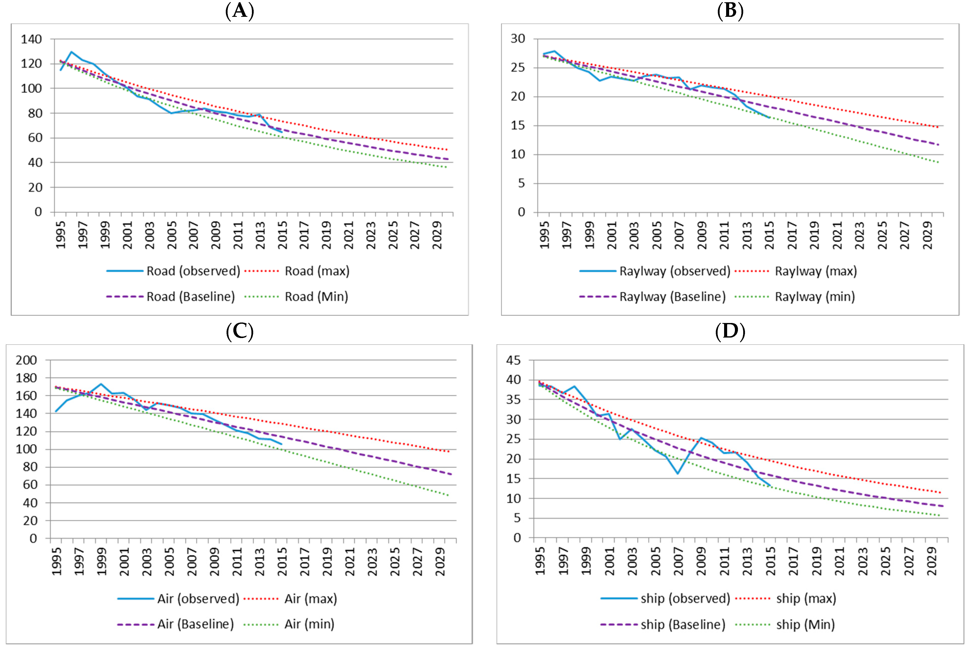
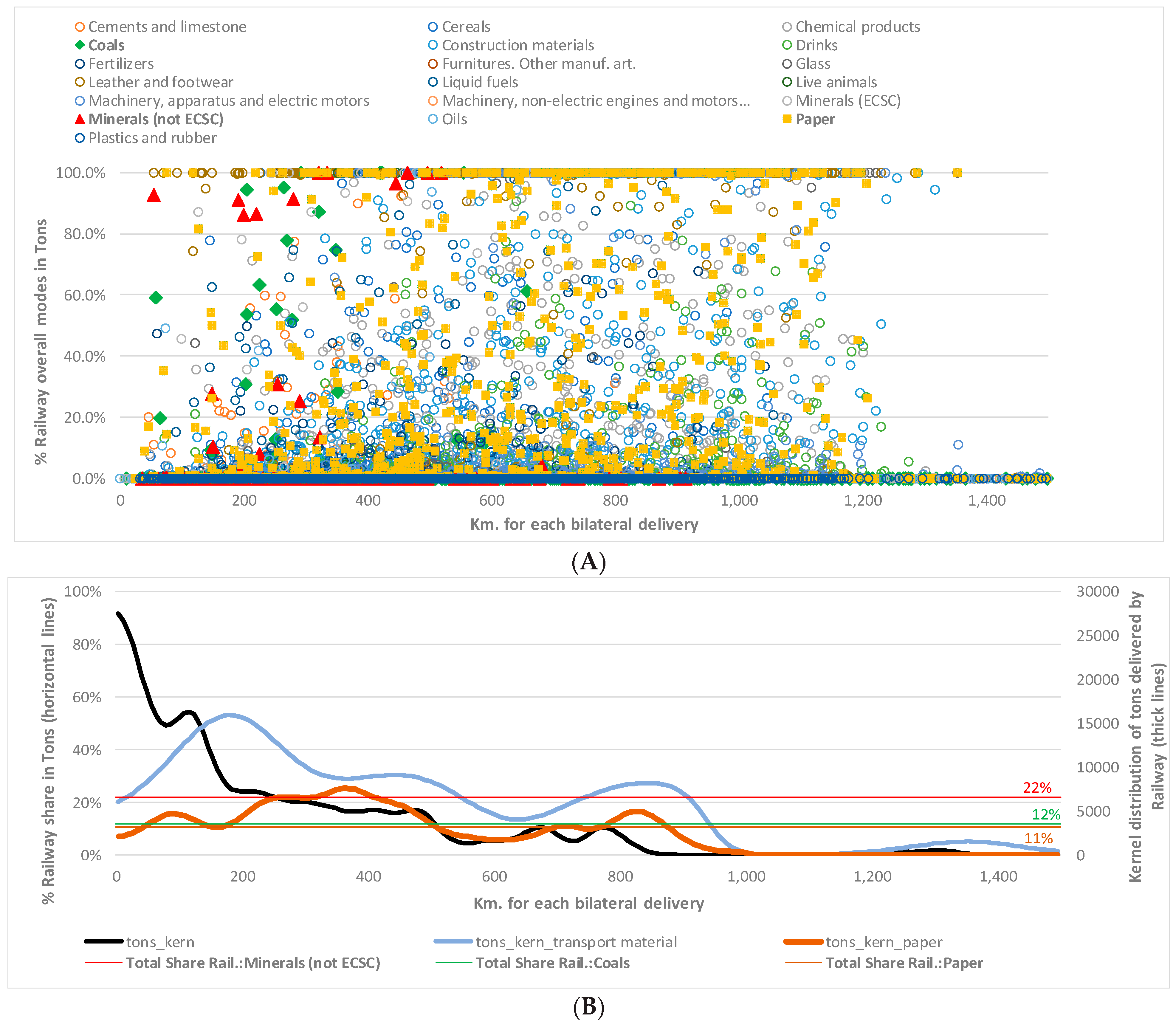