Combining Satellite and UAV Imagery to Delineate Forest Cover and Basal Area after Mixed-Severity Fires


1
Faculty of Environment and Natural Resources, University of Freiburg, Chair of Forest Utilisation, Werthmannstraße 6, 79085 Freiburg, Germany
2
Faculty of Environment and Natural Resources, University of Freiburg, Chair of Remote Sensing and Landscape Information Systems, Tennenbacherstr. 4, 79106 Freiburg, Germany
*
Author to whom correspondence should be addressed.
Sustainability 2018, 10(7), 2227; https://doi.org/10.3390/su10072227
Submission received: 11 June 2018
/
Revised: 22 June 2018
/
Accepted: 26 June 2018
/
Published: 28 June 2018
(This article belongs to the Section Environmental Sustainability and Applications)
Abstract
:In northern Argentina, the assessment of degraded forests is a big challenge for both science and practice, due to their heterogeneous structure. However, new technologies could contribute to mapping post-disturbance canopy cover and basal area in detail. Therefore, this research assesses whether or not the inclusion of partial cover unmanned aerial vehicle imagery could reduce the classification error of a SPOT6 image used in an area-based inventory. BA was calculated from 77 ground inventory plots over 3944 ha of a forest affected by mixed-severity fires in the Argentinian Yungas. In total, 74% of the area was covered with UAV flights, and canopy height models were calculated to estimate partial canopy cover at three tree height classes. Basal area and partial canopy cover were used to formulate the adjusted canopy cover index, and it was calculated for 70 ground plots and an additional 20 image plots. Four classes of fire severity were created based on basal area and adjusted canopy cover index, and were used to run two supervised classifications over a segmented (algorithm multiresolution) wall-to-wall SPOT6 image. The comparison of the Cohan’s Kappa coefficient of both classifications shows that they are not significantly different (p-value: 0.43). However, the approach based on the adjusted canopy cover index achieved more homogeneous strata (Welch t-test with 95% of confidence). Additionally, UAV-derived canopy height model estimates of tree height were compared with field measurements of 71 alive trees. The canopy height models underestimated tree height with an RMSE ranging from 2.8 to 8.3 m. The best accuracy of the canopy height model was achieved using a larger pixel size (10 m), and for lower stocked plots due to high fire severity.
1. Introduction
The assessment and recuperation of degraded forest is a great challenge for science and practice [1,2]. Furthermore, even when the most relevant international institutions have already proposed guidelines for the restoration of degraded lands [3,4,5,6], the definition of degraded lands is still in discussion by the most relevant international institutions [7], and it is in many studies addressed as a self-explanatory concept [8,9]. In the Argentinian Yungas, land use change into agricultural systems and forest degradation are driving the forest sector to a critical status due to the economical loss created by the low stock of wood products [10]. In order to plan adaptive forest management measures to recover forest stocks, an intensive assessment of those forest lands is necessary. The Yungas forest presents a complex structure [11,12,13], which is additionally diversified in mortality-patch size, species composition, and post-disturbance dynamics of surviving trees with fire-created coarse wood, when they are affected by mixed-severity fires, among other disturbances [14,15]. Mixed-severity fires are burns with a heterogeneous spatial distribution of high, moderate, and low severity [16], and have already been studied to identify stand-replacing patches on Landsat TM imagery [17]. However, with the objective of their assessment at a more detailed scale, identifying local indicators and thresholds is necessary. An intuitive approach is to consider the definition of a forest by the Argentinian Federal Council of Environment (COFEMA—2012) [18], which is used for the implementation of the Argentinian forest law 26331 [19]. It has set minimum thresholds of extension (0.5 ha) and canopy cover (20%) of a certain tree height (3 m) for a land to be considered a forest. Forest canopy cover and tree height are, furthermore, variables of great interest for the prediction of live basal area (BA), which has already been used to assess forests affected by mixed-severity fires [15]. Therefore, in order to delineate homogeneously degraded forest, this manuscript addresses fire severity based on the losses of forest stocks and productivity.
Attempts to assess canopy opening caused by selective logging [20,21,22] and wildfire [23,24,25] have been made with different satellite sensors [26,27]. However, those approaches have their limitations with respect to possible ground resolution, frequent cloud cover, and costs of the imagery [28,29]. Consequently, Frolking et al. [14] remarked that key hurdles in the use of satellite imagery, such as cloud cover and the detection of small-scale disturbed areas, have to be addressed. Several researches have calculated canopy height models (CHMs) from the combination of airborne laser scanning-digital terrain models (ALS-DTMs) and photogrammetric digital surface models (DSMs) [30,31,32]. CHMs derived attributes were correlated to forest attributes to conduct area-based inventories [33,34] and to assess disturbance damage [35]. However, in all those studies, a precise ALS-DTM was used, since photography does not allow the assessment of under-story vegetation and ground under dense canopy [36,37]. In this scenario, UAV technology appears to be very promising for the assessment of small scale diverse forest structure, since it offers a high acquisition flexibility and resolution at relatively low costs [38], but only if a precise DTM is available [39,40] or the forest is widely open [41]. Recently, Iizuka et al. (2018) [42] addressed this problem by comparing multiple settings to calculate photogrammetric DTMs for a Japanese cypress forest. Their best estimations were with a cell size of 60 m, maximum angle of 25°, and maximum distance of 1.3 m via adaptive TIN modelling.
All present methods to assess diverse forest by satellite imagery require validation of the data with a sample-plot-based field inventory, since the most accurate information can be achieved with a combination of the two data sets [43]. Alternatively, the use of UAV with optical or laser sensors has been shown to support forest inventories, but is limited to a low scale (100 to 1000 ha) [40,44]. Area-based inventories combine high-resolution, full-coverage, remotely-sensed data with ground information in order to predict forest attributes over the whole area [36,45]. For instance, Bohlin et al. (2012) [46] have conducted the area-based approach over a homogeneous forest, having an RMSE of 14.9% for the estimation of BA from aerial images. Other studies combine different scale source data. For example, Nelson et al. (2009) [47] combined six data sets (including ground plot, ALS, and Landsat imagery) to assess large-scale biomass stocks. Ene et al. (2016) [48] compared the precision of estimation of above ground biomass on a forest inventory supported with wall-to-wall and partial coverage ALS data. The results reported 10% major precision for the wall-to-wall coverage, but a much higher cost of acquisition. They recommended the use of low cost wall-to-wall data, such as satellite imagery, and samples from a more precise source, such as ALS or photogrammetric point clouds. This approach would overcome the problems of choosing either large scale or high-resolution imagery, and reduce the number of ground plots of highly demanding and dense field surveys. More recently, Puliti et al. (2017) [44] demonstrated the gains of the ’hybrid inference’ approach to improve the precision of volume estimations in forest inventory, combining ground plots with partial cover UAV imagery and ALS data. Fraser et al. (2017) [49] correlated Landsat spectral indices with UAV-derived metrics to assess forest severity in a boreal forest in Canada. Puliti et al. (2018) [50] used combined ground plots with partial cover UAV imagery and Sentinel-2 data on a hierarchical model-based inference to predict ground stock volume. After rigorous statistical analysis, they found similar estimates were obtained when comparing this approach (SE = 3.53%) and the area-based approach using ALS data (SE = 3.33%). However, most of the studies conducted to-date [32,34,37,44,46,49,50] have been over even-aged stands, reporting good estimations of canopy external structure. White et al. (2013) [36] recommended further studies analysing the limitation of using UAV image point clouds on area-based approach inventories applied to heterogeneously structured forests.
In order to evaluate how partial cover UAV imagery can contribute to the assessment of disturbed remote forest areas, this research aims to assess the quality of photogrammetric CHMs over a gradient of degradation of forest affected by mixed-severity fires in a case study in the Yungas Cloud Forest in northern Argentina. The second aim is to assess the feasibility of using those CHMs to support the stratification of forests in order to improve the accuracy of medium scale forest inventories by combining the partial cover of UAV imagery with wall-to-wall satellite images and ground inventory. These aims arise from the hypothesis that accurately training satellite image classification with partial cover UAV photogrammetric data would allow researchers to reduce the classification error of the wall-to-wall satellite images. Therefore, the first objective of this research is to assess the precision of photogrammetric CHM across a gradient of fire severity. The second objective is to compare the classification error of a same SPOT 6 image in four fire severity strata trained by two different data inputs: (1) BA from a plot-based forest inventory, and (2) BA from a plot-based forest inventory and CHM metrics calculated from partial cover UAV imagery.
2. Materials and Methods
2.1. Study Area
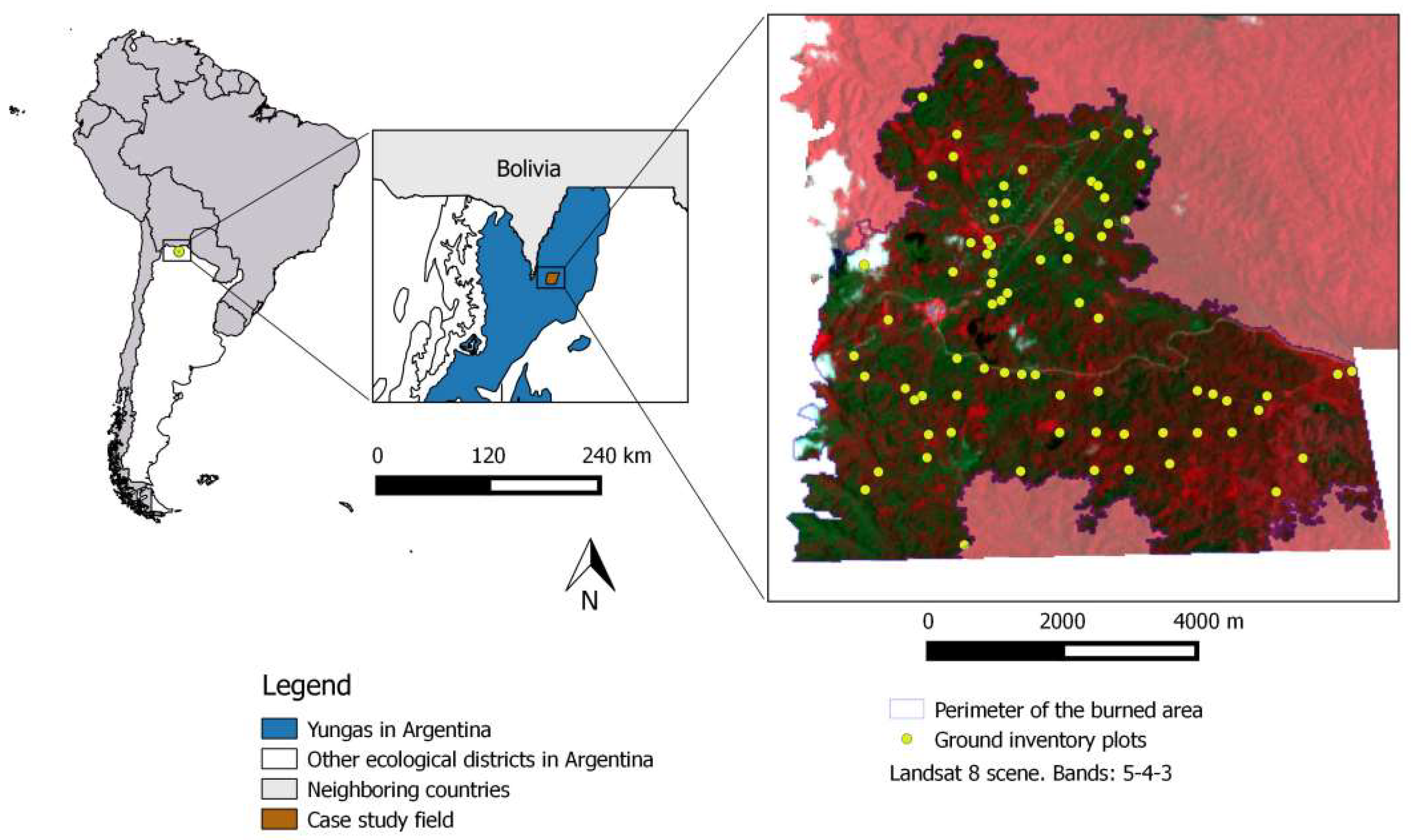
The study area (Florestoona forest) is a private native forest affected by mixed-severity fires in the temperate ‘Selva Pedemontana de Yungas’, 29 km to the Northwest from the city of Embarcación in the province of Salta, Argentina. Yungas Cloud Forest is a seasonal subtropical ecosystem located in the Argentinian north-western Andean mountains between 400 and 3000 m a.s.l. [51]. Northern Argentina represents the most southern part of this ecological district, which occupies a major area in Peru and Bolivia. In Argentina, it is latitudinally extended to 700 km from the provinces of Catamarca (29° S) through Tucumán, Jujuy, and Salta, to the border with Bolivia (22° S), but the maximum longitudinal extension is not greater than 50 km [52].
The case study is located in the northern piedmont, also known as the floristic district of ‘palo blanco y palo amarillo’, where woody lianas and annual vines are abundant. In Florestoona, intensive harvesting has been implemented for more than 100 years, causing the decrease of stock and the economic value of the forest [53]. Furthermore, recurrent fires have affected the area. The last one took place after an exceptionally dry season in November 2013, mainly affecting the area under intensive forest management. This fire affected 3944 ha in the cadastre area of interest, although some patches are left unaffected within this area. Before the fire, in 2008, a forest inventory was conducted in Florestoona, finding an average BA of 17.15 m2/ha [53] (Figure 1), which is higher than the actual average in the Yungas Pedemontana [54].
2.2. Plot-Based Field Inventory
A first delineation of the burned area was done on a Landsat 8 scene from 19 December 2013 [20,55]. In August 2015, in a pilot survey inventory, a total number of 24 plots every 200 m were set in six transects randomly located beside existing roads. Tree species, diameter at breast height (DBH, with diameter tape), tree height (with Vertex IV and Transponder T3 v.1.0), and observations of the plot and of the individual trees were recorded. The locations of the plots were recorded with differential GPS every second during five minutes, and corrected with the UNSA (Salta) station during post-processing. Two circular concentric subplots were measured: an inner subplot of 300 m2 for trees with a DBH value lower than 30 cm, and an outer subplot of 1000 m2 for trees with a DBH value of 30 cm or more. The inner subplot was adapted to 1000 m2 when the number of trees was lower than eight. This design combines the two concentric mixed radii plot design with n-tree sampling [56], having the advantage of being adaptive to tree density [57], and keeping the radii from the plot design recommended for the Yungas forest [54].
In order to obtain a target stratified relative estimation error lower than 20% (based on BA), which is prescribed for valid inventories in Argentina [54], a second survey was carried out in two stages (December 2015 and November 2016). During the first stage, an additional 23 plots were randomly located over a grid of 500 m, and during the second stage, 30 stratified plots were randomly located and measured. Plot size, shape, and information collected were equivalent to those from the pilot survey inventory. Additionally, at that phase of the inventory, within the stratified randomly located plots, 90 ‘reference trees’ (three per plot) were selected, and their displacement from the centre of the plot was measured with a vertex and compass. Those trees were later used to assess the prediction of tree height from the CHMs. The 77 measured plots (24 from the pilot survey and 53 from the second survey) covered a total area of 7.7 ha.
2.3. UAV Imagery Acquisition
In total, 31 UAV flights were conducted in December 2015 to acquire aerial images, using a fixed-wing UAV (eBee, SenseFly Ltd., Cheseaux-sur-Lausanne, Switzerland) covering 74% of the burned area. The filters of the employed consumer grade compact camera (Canon PowerShot S110, Canon Inc., Tokyo, Japan) were modified by the UAV provider to take pictures in the near infrared (NIR), red, and green wavelength ranges. Flight lines maintained a constant altitude of 284 m above ground level, preferably parallel to altitude isolines, and with an overlap of 75% side and forward [39]. Missions were planned in advance with the software eMotion 2.4 (SenseFly Ltd., Cheseaux-sur-Lausanne, Switzerland), either individually or as a group of flights. Groups were arranged based on the time consumption to cover the full areas in consecutive missions in order to avoid differences in weather conditions reflected on the images. Flights were conducted between 11:00 and 14:00, since the inclination of sun rays at that time of day has the minimal shade effect on the resulting images. Being equipped with three batteries and two chargers, up to six flights per day were feasible, although many flights were cancelled due to strong wind (speed higher than 6 m/s) in order to reduce branch movement and image blur, which would negatively affect key-points matching.
2.4. Workflow
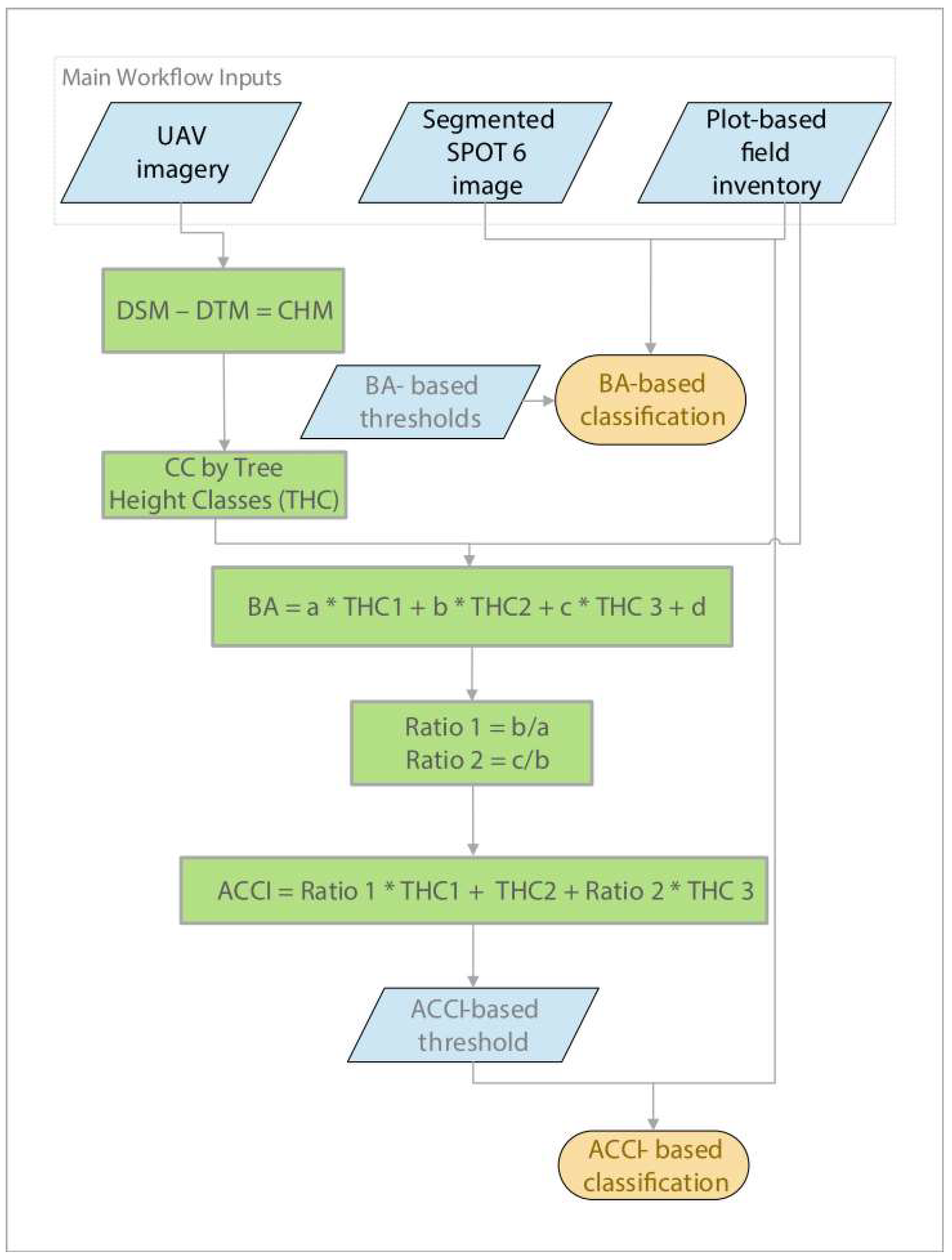
Figure 2 presents the workflow, which is further explained in the following subsections. After delineating the perimeter of the fire on a Landsat 8 scene, a SPOT6 multispectral image was acquired to conduct two supervised classifications into four fire severity strata (‘fully stocked’, ‘burned’, ‘severely burned’, and ‘very severely burned’). One of the classifications was trained with BA data from ground inventory data, and the other one with adjusted canopy cover index (ACCI) data. ACCI was formulated from the correlation of BA (from ground inventory) against partial canopy cover at three tree height classes (estimated from UAV-imagery derived CHMs). Cohen’s kappa coefficient and stratified estimation errors were compared to define whether or not including UAV-derived metrics improves the precision of the classification. In both classifications, part of the data was used as classification samples, but the whole dataset from the ground inventory was used to estimate classification errors (only one plot was excluded in this step because it was located outside the fire perimeter). For the first BA-based classification, 47 basal area data points from the plot-based field inventory were used to select classification samples [58]. For the ACCI-based classification, 64 samples were selected: 44 out of the 77 ground inventory plots, and an additional 20 image plots.
2.4.1. Photogrammetric Processing
UAV imagery has been attached with coordinates from the autopilot, and then further processed with the Structure from Motion (SfM) software Pix4discovery by Pix4D 3.1.22 [59]. The software, after several steps: interior and exterior camera calibration, image matching, and optimization (automatic aerial triangulation and bundle block adjustment), calculates a dense 3D-point-cloud (LAS file) and orthomosaic. Georeference of the scene was conducted directly based on GPS information attached to the picture files from the UAV-GPS device [60].
Point clouds were processed in the ArcGIS 10.3 environment to convert the LAS dataset to raster files by employing the void fill method ‘natural neighbour’ [61]. A single DSM and two DTMs were calculated: the DSM with a 0.5 m/pixel resolution, one DTM with a 5 m/pixel resolution (DTM5), and a second one with a 10 m/pixel resolution (DTM10). For computational efficiency, all data were resampled, to the same resolution of 0.5 m/pixel using the ‘nearest’ resampling method. Two CHMs were calculated as a result of deducting the resampled DTMs from the DSM. One was calculated using the DTM5 (CHM5), and the other using the DTM10 (CHM10). The accuracy of the CHMs was later compared based on ground measurements of ‘reference trees’ heights [35,42].
2.4.2. Tree Height and Adjusted Canopy Cover Index
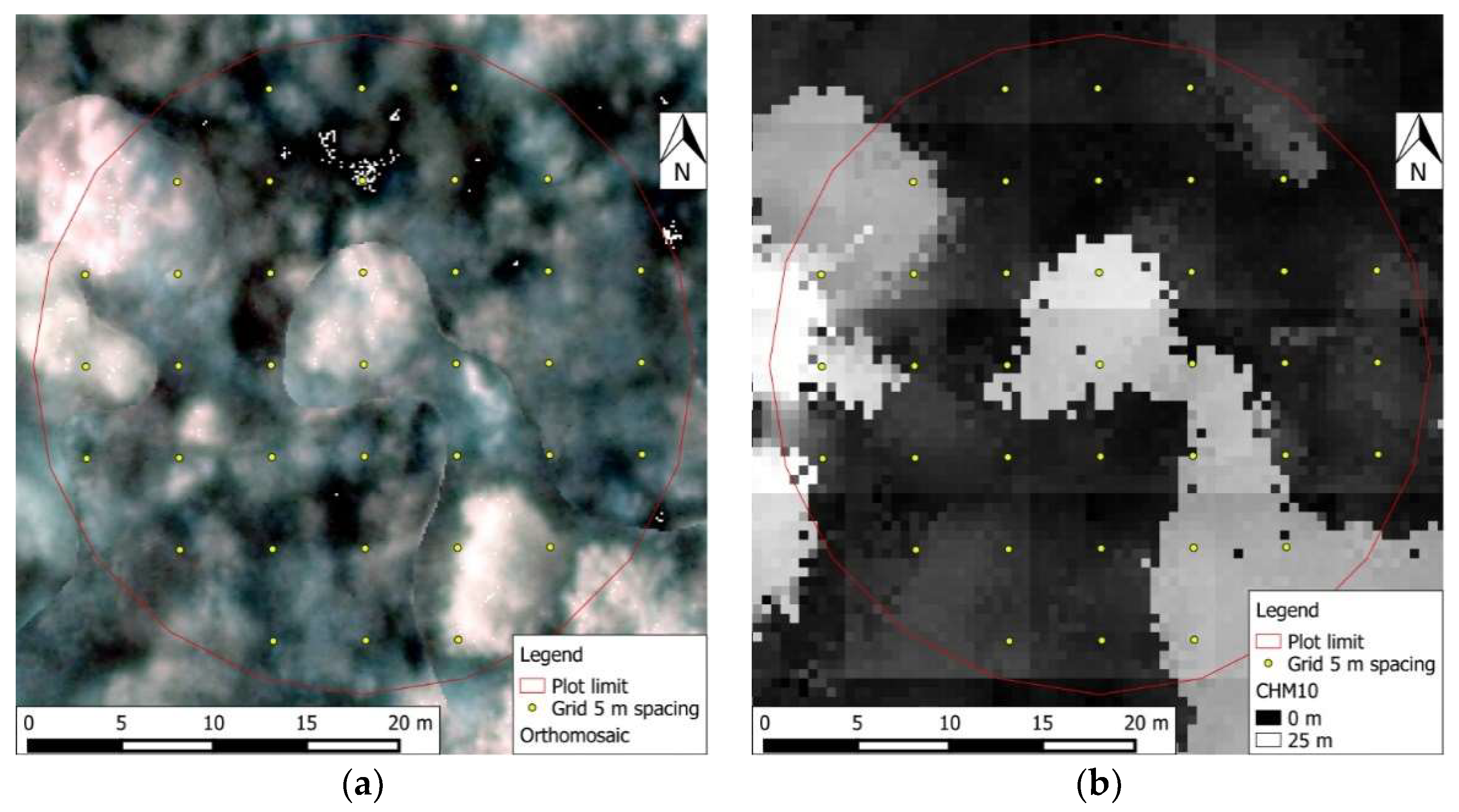
Canopy cover (CC) was calculated from CHM10 (Figure 3) at ground inventory plots. Grids of 37 points spaced every 5 m, and covering 100 m2, were created in order to have a reduced number of data, and feasibly control the data in cases of dense canopy cover producing pixelation. Since it is expected that CC from tall trees has a greater effect on BA than CC from shorter trees, forest vertical structure was stratified into three tree height classes (THC). Partial CC was calculated for 70 plots out of the 77 from the forest inventory (seven were excluded due to image blur):
- THC1: CC from tree heights between 5 and 10 m
- THC2: CC from tree heights between 10 and 20 m
- THC3: CC from trees higher than 20 m
Trees under 5 m were ignored in order to avoid accounting shrubs as trees. Nurminen (2013) [35] proposed this filter using a height threshold of 2 m, but in this study, it was adapted to 5 m, since it better represents the site conditions.
BA was correlated against partial CC through multiple linear regression using the software R 3.4.2 [62], as shown in Formula (1):
BA = a ∗ THC1 + b ∗ THC2 + c ∗ THC3 + d
In Formula (1), BA is the basal area of the given plot; ‘a’, ‘b’, ‘c’, and ‘d’ are the constant coefficients of the independent variables. Independent variables express partial CC at every THC: THC1 (CC from tree heights between 5 and 10 m), THC2 (CC from tree heights between 10 and 20 m), and THC3 (CC from trees higher than 20 m).
Coefficients ‘a’, ‘b’, and ‘c’ are a measure of the effect of the variables THC1, THC2, and THC3 on the prediction of BA, respectively [63]. For example, assuming that the other variables are constant, a change in one unit on THC1 will increase the predicted value of BA by a m2. Since independent variables scales are identical (all range from 0 to 100), the impact of the tree height classes on BA can be compared directly [64]. The transformation of the model by dividing the coefficients by ‘b’ gives three new ratios; one of those (b/b) is equal to one, and therefore, can be discarded. The other two ratios express the importance of THC1 and THC3 in comparison with THC2 based on the estimation of BA (Formulas (2) and (3)).
Ratio1 = a/b
Ratio2 = c/b
In Formulas (2) and (3), ‘a’, ‘b’, and ‘c’ are the coefficients of the independent variables THC1, THC2, and THC3, respectively, taken from Formula (1).
The formulated ratios weight the influence of every THC canopy cover on BA. Therefore, those ratios are used in Formula 4 to model ACCI (adjusted canopy cover index), abstracting the model from BA based on the ACCI-based classification. ACCI is formulated as an alternative to CC, which weights partial CC from tree height classes by their influence on forest stocks (BA). ACCI approaches the prediction of fire-induced damage, since it refers to horizontal and vertical structures of a stand and their influence on stocks.
ACCI = Ratio1 ∗ THC1 + THC2 + Ratio2 ∗ THC3
In Formula (4), ACCI is the adjusted canopy cover index, which represents the sum of the partial CC per the three height classes weighted by their effect on BA. Ratio1 and Ratio2 are the ratios of coefficients (Formulas (2) and (3)). THC1, THC2, and THC3 are the independent variables which express the partial canopy cover at every tree height class.
ACCI was calculated for the 70 ground plots and an additional 20 stratified image plots were randomly located over the area with UAV imagery cover.
2.4.3. Image Classification
An orthorectified SPOT6 multi-spectral image from 26 October 2014 was acquired to sort the two nearest neighbour image classifications into four forest strata of fire severity and bare land (for roads and buildings). This SPOT6 image was the first of its kind which, after the fire incident, had an acceptable cloud cover (<2%) over the area of interest. The nearest neighbour method consists of multiresolution segmentation and supervised classification, which were conducted with the software e-Cognition 9.2 [65]. This procedure has proven benefits, such as incorporating spectral and textural information, and therefore has been broadly used in environmental studies [66]. The scale parameter for segmentation was set to 10, image layers were all equally weighted, and heterogeneity criteria were set to 0.3 for shape and 0.5 for compactness.
In order to train and compare the two classifications, two sets of multiple thresholds of fire severity were defined [67,68]. A set of thresholds was based on BA data, and the other one was based on ACCI, in order to assess the contribution of UAV-derived metrics tn the classification of the SPOT6 image (Table 1). Strata of fire severity were defined assuming that forest stocks were uniform before the fire. Therefore, low forest stocks were related to severe fire damage. This assumption was based on the inventory carried out in 2008 [53], and on the fact that Florestoona belongs to the same phytogeographical area of ‘Selva Pedemontana de Yungas’ [52]. From the data of the 2008 inventory, the BA-benchmark of a fully stocked forest was set to 18 m2/ha, and the ACCI-benchmark was assigned arbitrarily to 100. The minimum threshold of a fully stocked forest was based on the recommendation for the sustainable management of native forests in the Yungas, which establishes that a minimum of two-thirds of the original BA (12 out of 18 m2/ha) should be left after a regular harvest [54]. The threshold values used to define the other classes were also established as thirds of the benchmark, with the objective of creating homogeneous ranges. However, the less stocked third was additionally divided into two classes, since a piece of land must have 20% CC to be considered a forest [18]. This criteria was extrapolated to the BA-based thresholds in order to get comparable results. An overview of the orthomosaics of the four fire severity and bare land strata is shown in Figure 4.
Two supervised classifications of the same segmented SPOT6 image were conducted using the software e-Cognition based on the BA-based and ACCI-based thresholds. To supervise the classification, segments over imagery and ground plots were assigned to classes. Samples of an additional stratum called ‘bare land’ were selected over roads and construction areas (houses, sheds). For the BA-based classification, samples were selected over the first 47 inventory plots. For the ACCI-based classification, 64 samples were selected: 44 out of the 47 plots used for the BA-based classification (three had to be excluded due to image blur), and the additional 20 image plots. The rest of the 12,991 samples were assigned to the closest class, based on their similar texture and spectral data from the SPOT6 image.
In order to compare the accuracy of the two methodologies used to stratify the forest, overall classification errors were calculated using Cohen’s kappa coefficient (k). This statistic uses a matrix of frequencies of predicted and actual stratum to calculate the agreement between them [69,70]. Standard error (SE) was calculated, and statistical difference between the k coefficients was assessed with a two sample Z-test and 95% confidence. Furthermore, stratified estimation errors and relative estimation errors were estimated using the BA from a total of 76 plots (one was excluded due to being located outside the fire perimeter), based on Formulas (5) and (6) [71], respectively. Statistical differences of the mean BA were tested with the use of the Welch t-test on the statistics software R 3.4.2 [62] with a confidence level of 95%. Welch t-tests can be used to compare mean differences in case the sample sizes of groups to compare are small and the variances are not homogeneous [71].
where E is the estimation error; S is the standard deviation of the BA from all the plots of the fire severity stratum; t is the t-value with 95% confidence in a two-tailed test; and n is the number of plots in the stratum.
where E % is the relative estimation error; E is the estimation error; and x̅ is the average BA from all the plots in the stratum.
E = (S*t)/n1/2
E % = (E/x̅) × 100
Finally, the number of plots necessary to achieve the target stratified estimation error of 20% was calculated with Formula (7) for each of the classifications.
where n is the number of plots used to achieve the stratified estimation error of 20% (0.2); t is the t-value with 95% confidence in a two-tailed test; and S is the standard deviation of the BA from all the plots of the fire severity stratum.
n = (t*S/0.2)2
2.4.4. Validation of CHMs
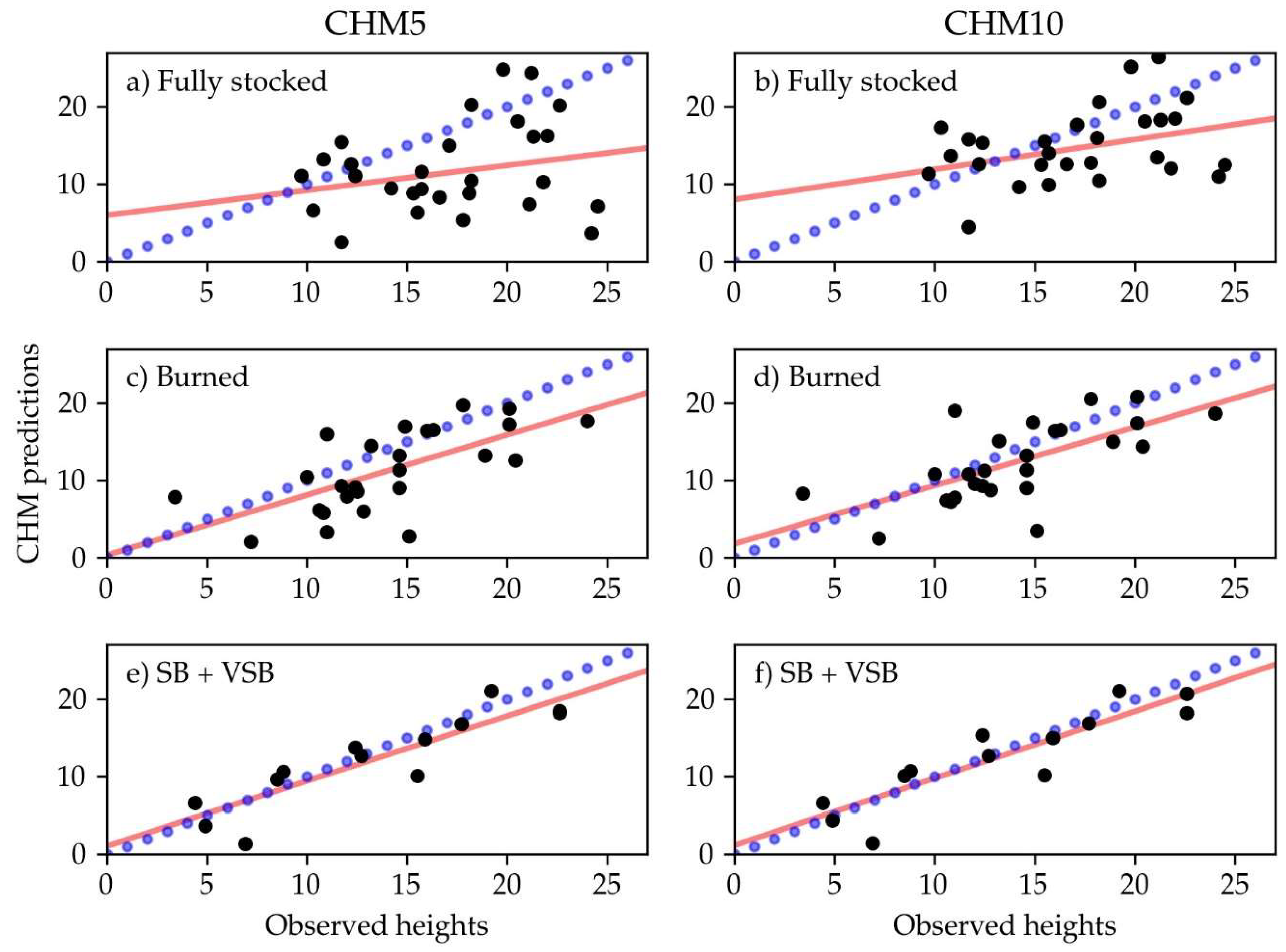
The ‘reference tree’ heights measured on the ground were correlated with their predictions from CHMs. Dead trees were eliminated from the analysis, since they were not properly detected by the cameras, and only live BA was counted. After this filter, 71 reference trees remained for the correlations. Most of the excluded trees were located on the two most degraded strata, leaving only 13 trees in the two least stocked strata. Therefore, the correlations of the tree heights measured on the field and their estimations from CHM5 and CHM10 were conducted by three groups: (1) fully stocked, (2) burned, and (3) severely burned (SB) together with very severely burned (VSB). Mean absolute error (MAE), RMSE, and coefficient of determination (r2) were calculated for both CHMs and fire severity strata.
3. Results
3.1. UAV Image Acquisition
Two out of the 31 UAV flights were discarded due to incorrect GPS data attachment on the single images, resulting in 3801 images, which covered 2915 ha. In total, 18 GeoTIFF orthomosaics were created according to the groups of flight planning, with a ground resolution of 11.78 cm/pixel, although flights had been planned with a ground sampling distance of 10 cm/pixel. This small variation was expected due to the low precision of the available DTM used for flight planning, terrain altitude variations on the same flight line, and error in GPS positions. During image processing, for 2-D bundle adjustment, an average of 0.42 key points/m2 was used, and 0.19 key points/m2 for 3-D bundle adjustment. Point cloud densification was obtained with an average of 8.32 points/m2.
3.2. Photogrammetric Processing
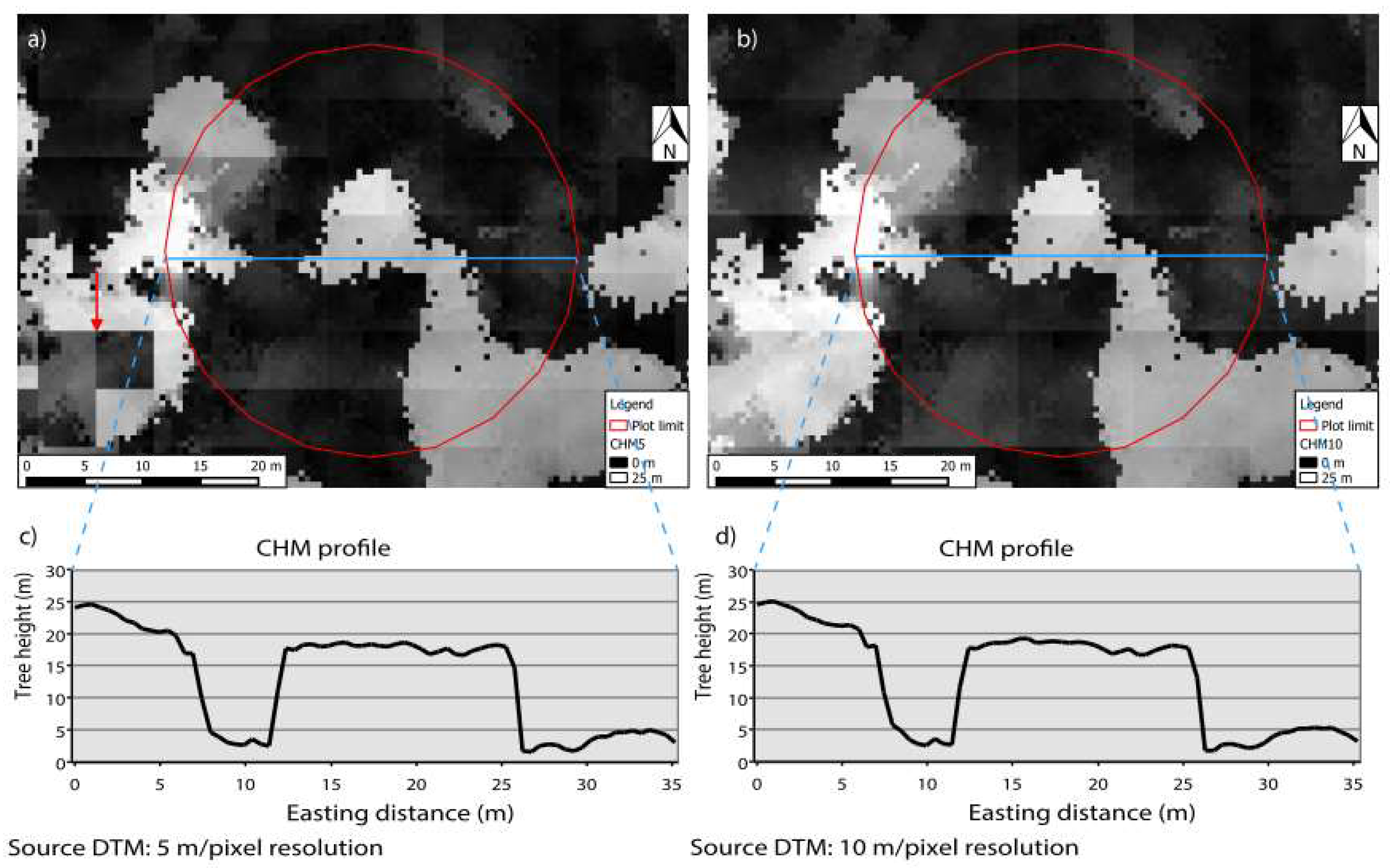
Small differences between the CHMs were observed in areas of open canopy, as shown in Figure 5, where a CHM5 and a CHM10 profile along a transect of an example plot are compared. Tree heights are underestimated when DTM is calculated from shrubs or low canopy points, instead of actual terrain. A broader filter improves the accuracy of DTM, since the selection of the points is more likely related to terrain on canopy gaps. The errors of DTM5 and DTM10 are then extrapolated to CHM5 and CMH10. The red arrow on Figure 5 points to an example error on the CHM5, where an abrupt change of canopy height on the model is evident.
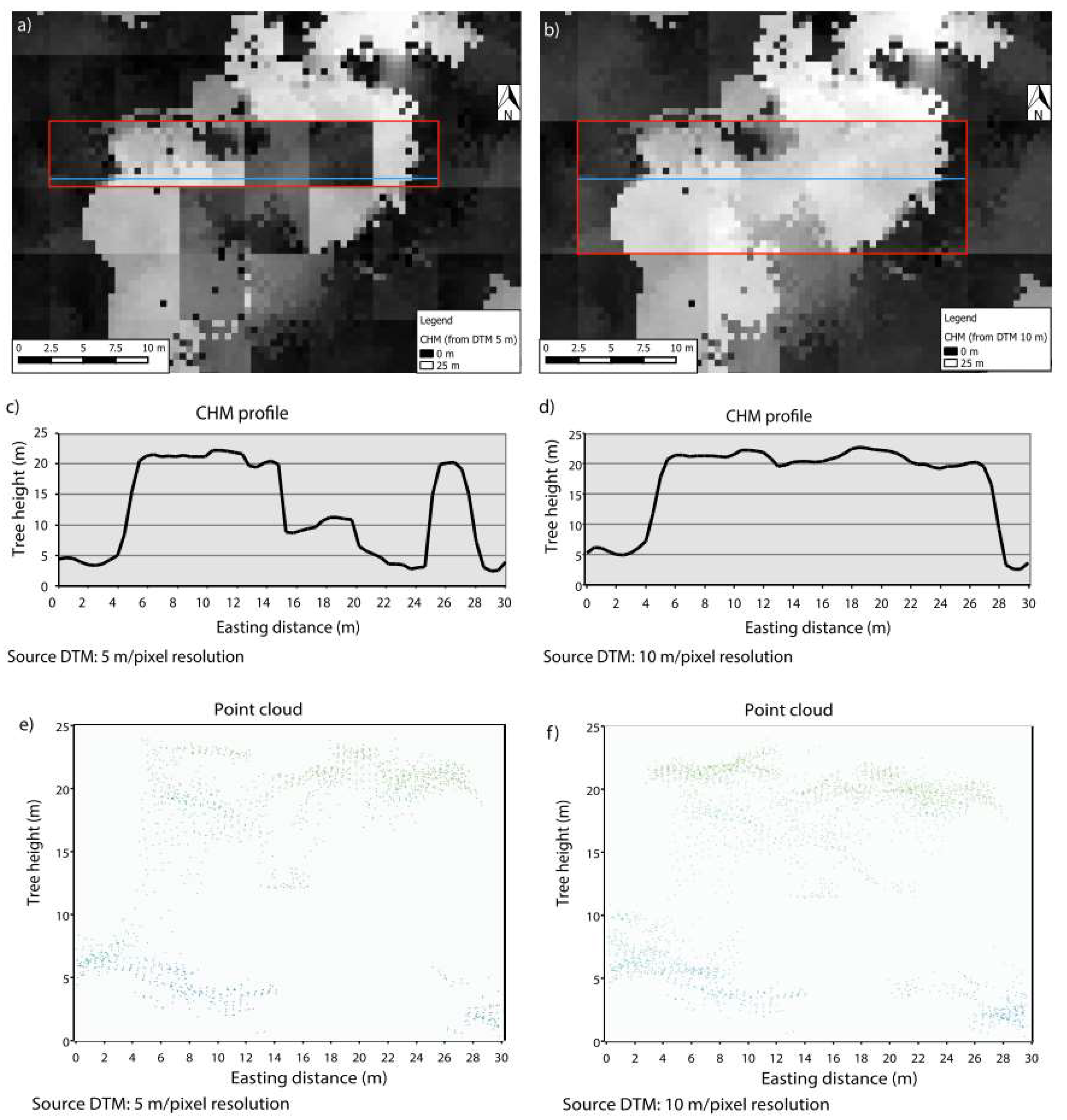
Figure 6 shows, in detail, the example error caused by the lack of key points from terrain, as presented in Figure 5. A transect of 30 m (from west to east) along a pixelated area is analysed on each of the CHMs. In Figure 6a,b, CHM5 and CHM10 of the same area are shown. Figure 6c shows the profile of the calculated CHM5. Every five meters, changes in the source DTMs used for its calculation reflect differences in comparison with the CHM10 shown in Figure 6d. The greatest difference between the profiles is presented in the range of easting distance of 15 m and 25 m, where a great pixelation is observed on the CHM5. It is coincident to the point cloud, where no low key-points were obtained during image matching for these distances (Figure 6e,f). These differences are due to the obstruction of the terrain caused by a dense canopy above this area. This error is solved using lower resolution DTM (10 m/pixel instead of 5 m/pixel).
3.3. Tree Height and Adjusted Canopy Cover Index
In several cases, relatively big live patches of forest with dense canopy cover also produced errors (evident by pixelation) in the calculations of CHM10. Abrupt changes of tree height on CHM were always confirmed through visual inspection on the corresponding orthomosaic. When an error due to dense canopy cover was confirmed, the nearest tree height was manually extrapolated to the analysed point of the CC-grid.
The outputs of the multiple linear regression used to estimate BA by the independent variables THC1, THC2, and THC3 are shown in Table 2, and the model in the Formula for BA. This model has an adjusted r2 of 0.76, and all the independent variables have a significant influence with more than 99% confidence.
BA can be predicted from the partial CC at every THC (BA = 0.14742 × THC1 + 0.22734 × THC2 + 0.32320 × THC3 − 0.93010). Ratio1 (THC1/THC2) = 0.648 expresses that canopy cover from THC1 has a 35.2% lower impact on the BA than that from THC2. Ratio2 (THC3/THC2) = 1.422 expresses a 42.2% stronger impact of THC3 on BA than THC2. ACCI is then calculated by Formula 8.
where THC1, THC2, and THC3 are independent variables; the number 0.648 is Ratio1; and the number 1.422 is Ratio2.
ACCI = 0.648 × THC1 + THC2 + 1.422 × THC3
ACCI and BA are plotted on Figure 7, which shows the thresholds for the definition of strata of fire severity based on ACCI thresholds used for the image classification.
3.4. Image Classification
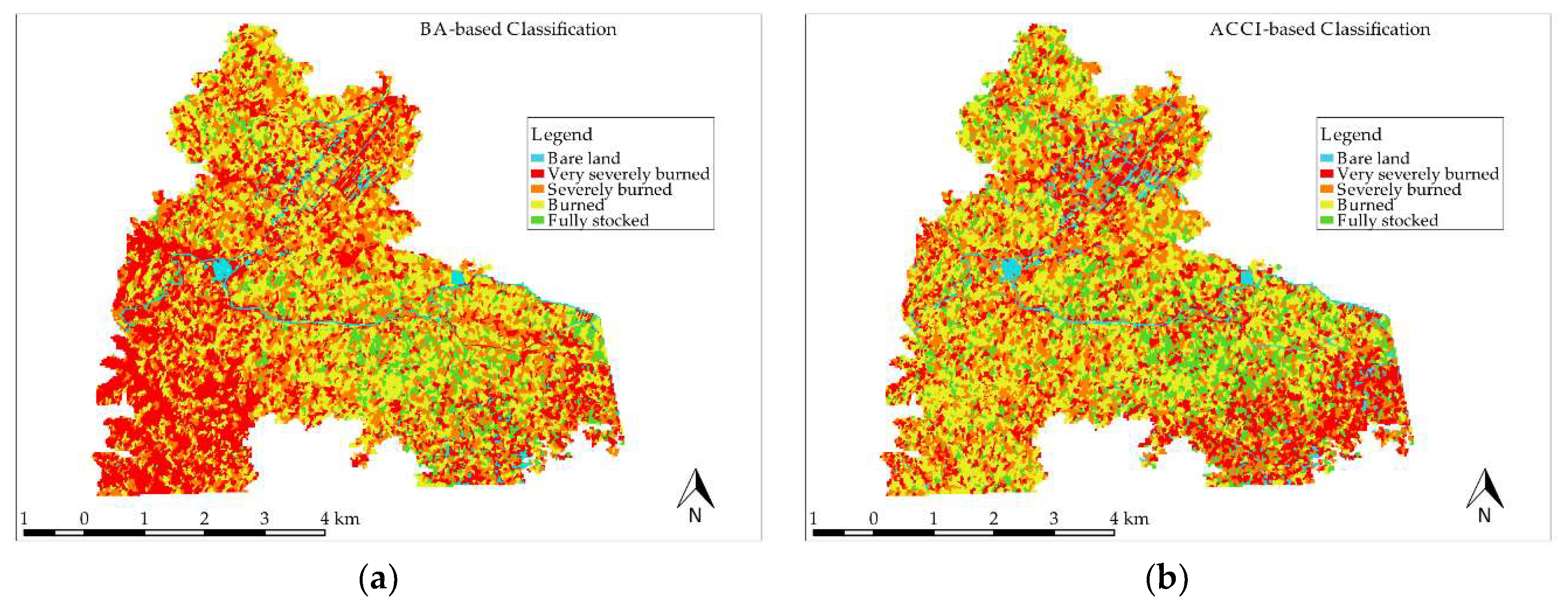
Image segmentation resulted in 12,991 polygons of an average of 3036 m2 from a total area of 3944 ha. Figure 8 shows the maps of both classifications of the SPOT6 image (BA-based and ACCI-based).
The matrices used for the calculations of the Cohan’s kappa coefficient (k) are reported in Table 3. The overall accuracies of the classification show no statistically significant differences (p-value: 0.43): k of 0.60 (69.7% of the plots correctly predicted, SE: 0.04) in the BA-based classification, and 0.55 (67.1% of the plots correctly predicted, SE: 0.04) in the ACCI-based classification. Table 4 reports and compares the results of the classification with the classes SB and SVB joined as a unique class, representing the least stocked third. For all the strata, the relative estimation error is lower in the ACCI-based classification and lower than the target of 20% for the strata ‘burned’ and ‘fully stocked’. However, the most damaged third (VSB + SB) presents a stratified relative estimation error over the limit of 20% (as it is prescribed for inventories in Argentina) in both classifications. Since the calculation of relative error is based on average BA, low average BAs are more sensitive to changes in estimation errors [63].
The results of the least stocked third are then separated into the strata ‘very severely burned’ and ‘severely burned’ (Table 5). Dividing the least stocked third into the classes VSB and SB was necessary for two reasons: (1) to reduce the influence of low values of BA on the whole class by having two more homogeneous strata; and (2) to identify and isolate those areas under 20% of ACCI (closely related to CC), since it is a threshold for the definition of a forest under Argentinian law. The amount of area assigned to each of the strata is similar for both classifications, except for a difference of around 300 ha between the most and the least stocked strata (Table 4). For the BA-based classification, 2191 ha are assigned to the least stocked third, corresponding to 1237.6 ha of the stratum VSB and 953.4 of SB (Table 5). For the most degraded third, only slight differences were reported between the classifications in terms of area classified as SB. However, a great difference can be appreciated for the stratum VSB. This can be explained by the results reported in Table 3, which show that of nine plots predicted as VSB in the BA-based classification, three were actually fully stocked. The stratum VSB has low stocks, leaving open areas for the colonisation by grass and vines [1,54,72]. A misclassification of stands between the strata VSB and ’fully stocked’ can be observed, probably due to the similar spectral characteristics that those strata display [73]. ACCI-based classification, since it takes information from canopy cover, has achieved a reduction of misclassified areas due to similar spectral responses of grass (and vines) and fully stocked forest. From the ACCI-based classification, homogeneous strata with a reduced number of outliers, and a relative estimation error lower than 20%, were achieved for all the areas with an ACCI value higher than 20. Table 4 and Table 5 also report the number of ground plots required to achieve the target error. For the BA-based classification, 28 and 17 additional ground plots would be necessary in order to achieve the target error for the classes SB and ‘fully stocked’, respectively; whereas no additional plots are necessary for the ACCI-based classification.
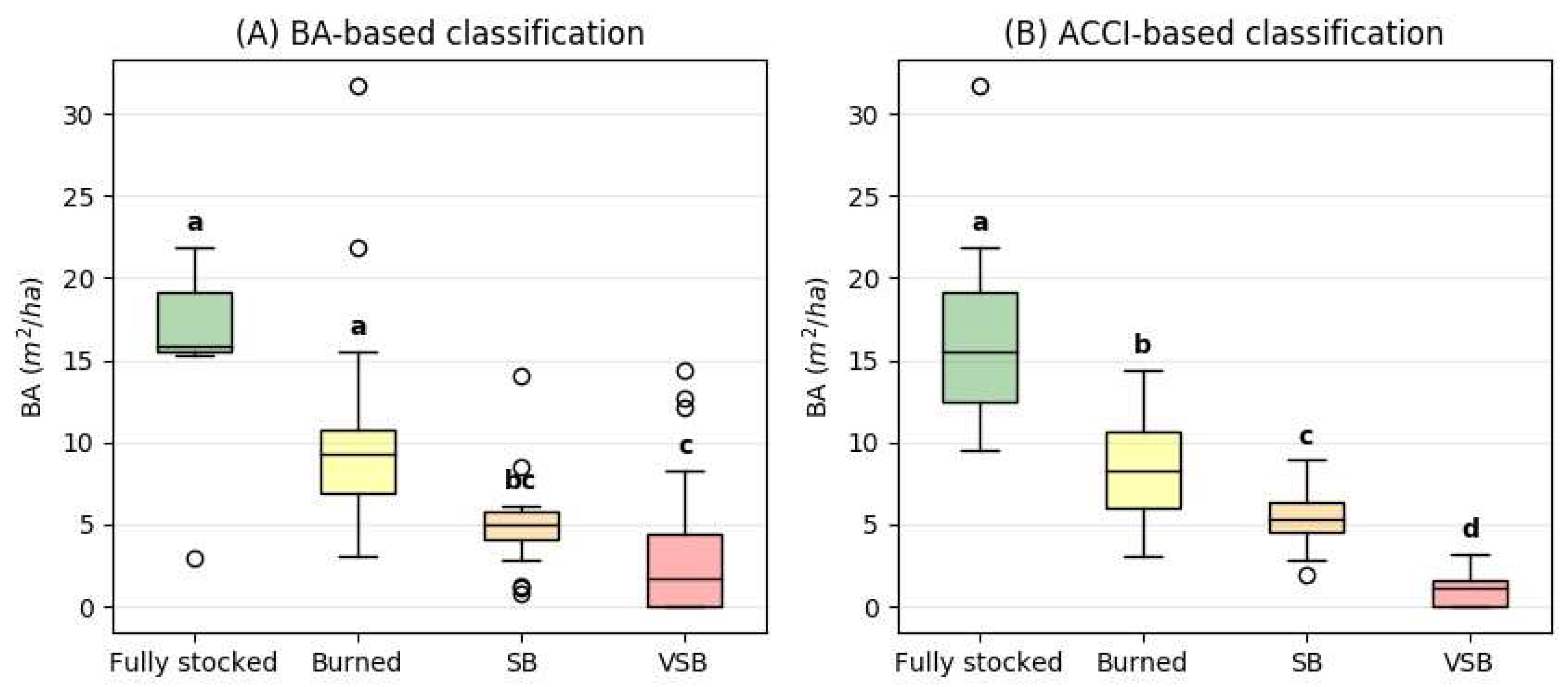
Statistically significant differences can be seen between all the strata from the ACCI-based classification, but only between the two middle strata from the BA-based classification (Figure 9). The better precision of the ACCI-based classification in comparison with the BA-based classification, might be due to a larger number of training areas used to run the classifications (64 and 47, respectively), and to the detection of misclassified areas with a similar spectral response. This is one of the main outputs of this research, because having used the same number of ground plots, more homogeneous strata were achieved by additional samples of UAV imagery, for which only ACCI values were calculated.
3.5. Validation of CHMs
Coefficient of determination, RMSE, and mean absolute error of the correlations of tree heights measured on the ground against their estimation from CHM5 and CHM10 are shown in Table 6. Graphs of correlations are shown in Figure 10, discriminated by strata, and by CHM5 and CHM10. For all the analysed strata, tree height is underestimated. This might be due to the limitation of optical sensors to reach data under the canopy, and low vegetation. The more severe the fire, the lower the obstruction caused by the forest canopy and, consequently, the lower the estimation error. The reduction in the estimation error is also evident for CHM10 in comparison with CHM5.
4. Discussion
In this research, the assessment of fire severity is addressed by damage to the forest canopy and the reduction of forest stocks [21]. Whereas reflectance data of the forest were acquired from the SPOT6 image and used for its segmentation and classification, photogrammetry-derived structure attributes (CC and tree heights) were calculated from UAV imagery, and correlated with BA acquired from the ground inventory. The correlation of partial canopy cover at three tree height classes against BA had an r2 of 0.76, the same as the results found by Bohlin et al. (2012) [46], but higher than the ones of Puliti et al. (2015) [34], who obtained prediction of BA with an r2 of 0.60 using an ALS-derived DTM. Fraser et al. (2017) [49] also obtained less promising results using UAV and Landsat imagery derived spectral indexes to predict the Composite Burned Index (CBI), as an indicator of fire severity, with an r2 between 0.36 and 0.6. However, they found r2 between 0.69 and 0.81 when comparing the indices they formulated from both remote sensors (UAV and Landsat imagery), which is better than the correlation to CBI estimated on the ground. In this research, the good prediction of ground data might be attributed to the higher number of field plots, as well as the use of tree height classes and not only total CC. These results allowed the use of ACCI as a prediction of forest stocks without the need for expensive ALS equipment. ACCI is presented in this research as an alternative to CC to define classes of fire damage, weighting CC from tree height classes by their influence on forest stocks (BA). In this context, ACCI was shown to achieve a good prediction of fire-induced damage to forest stocks, equating to forest economical degradation, since it refers to horizontal and vertical structures of a stand and their influence on growing stocks [15]. The final aim of this research was to delineate homogeneous stands of a forest area with fire-induced heterogeneous stocks in order to plan their rehabilitation; therefore, pre-fire stocks were considered homogeneous along the forest [49,67,68]. The proposed methodology has proven to be a powerful tool to delineate forest stocks after fire, but only when the forest is open enough to allow the sensors to get information about the terrain elevation.
An area-based approach to conduct forest inventories is structured in two steps: in the first step, ground and remotely-sensed data are correlated; in the second step, the predictive models are applied to a wall-to-wall cover [33,45]. Responding to the recommendations of Ene et al. (2016) [48], the presented methodology added a third step, since three source data scales are available: local (ground plots), partial cover (UAV imagery), and wall-to-wall cover (satellite image). Adding strategically localised UAV flights to a plot-based field inventory allowed us to correlate field data with UAV-derived metrics. Therefore, the supervision of satellite image classification could be conducted in areas where no ground data was available, but only UAV-imagery. This methodology achieved a reduction in the number of outlier misclassified stands in comparison with the approach where only ground data was used for supervision. Therefore, the stratified BA-based estimation error from the classification could be achieved by additional image plots without the need for a higher number of inventory plots, which are costly to conduct. In the present case study, the desired BA-based error was achieved with an additional 20 image plots, but depending on the objectives of the inventory, more image plots could be calculated on UAV imagery in order to improve image classification further. From another perspective, Puliti et al. (2018) [50] demonstrated that adding wall-to-wall Sentinel-2 data to an inventory conducted with partial cover UAV imagery and ground plots drastically decreases the need for UAV cover.
Regarding the accuracy of the estimation of tree heights, three different cases must be separately analysed. The first one when the ACCI value is higher than 66 (which relates to the stratum ‘fully stocked’). The estimation of individual tree height by the CHM5 without any human supervision has a mean absolute error of 6.8 m, and the adjusted coefficient of determination from the correlation of the observed and estimated individual tree height is insignificant (0.06). The predictions have a better approach when the CHM10 is used (MAE: 4.54 m, r2: 0.12), but are still not satisfactory. In general, for dense canopy cover forest areas, the results have confirmed the findings of Dandois and Ellis (2010) [39]. In those cases, it is better to count with another source to calculate a precise DTM, because the errors are extrapolated to the calculation of CHM. However, in these cases of dense canopy cover, orthomosaics have been used to identify the causes of the pixelation through visual inspection, and to manually correct it while estimating partial CC pat the THC. The second case is for the stratum ‘burned’ (with ACCI values between 33 and 66). The results found for this stratum (r2: 0.44, RMSE: 4.20 m) are comparable to those found by Dandois and Ellis (2010) [39] using UAV imagery to estimate the surface model and DTM for ALS data (r2: 0.53, RMSE: 4.31 m). More accurate predictions were found by the same authors using DTM calculated from UAV imagery (r2: 0.64, RMSE: 3.76 m). In this case, the authors attributed the error to a possible GPS limitation at calculating altitudes, and to the obstruction of the view to calculate DTM under dense canopy cover. Correcting those limitations by the use of GCPs (ground control points), the same authors reported better results in another experiment for both cases, with DTM from UAV imagery (r2: 0.74, RMSE: 3.28 m) and from ALS data (r2: 0.8, RMSE: 2.88 m). Those values corrected with GCPs, and the use of ALS data for calculating DTM, are similar to the findings in this research for areas with an ACCI value lower than 33 (third case of analysis), where the r2 of the correlation between observed and predicted tree heights is 0.79 and 0.8 for CHM5 and CHM10, respectively. RMSEs are also similar to the ones found by Dandois and Ellis (2010) [39]: 2.96 m and 2.85 m for CHM5 and CHM10, respectively. However, Lisein et al. [30] achieved better estimations of individual tree heights using DSM from UAV, and DTM from ALS, with significantly better precision (r2: 0.91, RMSE: 1.04 m). Those authors also found a correlation of 98% between CHM from UAV and ALS data when using the same DTM model for the calculations. Additionally, more promising results were found by Wallace et al. (2016) [37], who estimated CHM in relatively open Australian forest with an RMSE of 1.3 m. However, in this case, the study area was only 1500 m2, and the flight altitude only 30 m above ground level, catching 425 images for the area. Such intensive acquisition of images is not feasible at the field scale of the present research. The same authors mentioned a reduction of precision at a higher flight altitude, and under dense canopy covers. In summary, better precision was obtained when the canopy cover of the stands was lower. Those limitations are coincident to Wallace et al. (2016) [37] and Dandois and Ellis (2013) [41], who calculated more accurate DTM in sparse forest than in areas with dense canopy cover.
The use of UAV imagery to assess canopy cover is usually recommended only if a detailed terrain model is available, since the DSM only penetrates the terrain if there are gaps in the forest [32], as dense canopies limit the assessment of under-story objects [33,34,35,36,37,38,39,40,41,42,43,44,45,46,47,48,49,50,51,52,53,54,55,56,57,58,59,60,61,62,63,64,65,66,67,68,69,70,71,72,73,74,75,76]. In Argentina, the available DTM has a resolution of 30 m/pixel with an error of 3 m in altitude, which is far less precise than those of lower than 1 m horizontal and 0.15 m vertical resolutions in some developed countries [26,77]. However, from this research, a step forward in the assessment of fire-induced open forest areas was achieved. The use of UAV technology was used for the assessment of a fire-induced open forest where no precise high-resolution DTM was available. Supervision was needed to estimate tree height accurately, since dense canopy cover caused error in the automatic calculation of CHMs. The lower resolution DTM (10 m/pixel) proved to avoid many errors in the estimations of the CHM, which are frequently observed (by pixelation) on the CHM5. A bigger spacing for their calculations increases the chance to reach data closer to the actual terrain, although this gain in precision is obtained at the expense of a lower resolution. For the example of the case study area, this methodology allowed an increased resolution of the DTM, from 30 m/pixel to 10 m/pixel, keeping the same expected vertical error (3 m) from the available SRTM-DTM for the stands with an ACCI value lower than 66. Furthermore, those errors can be reduced if a high precision and resolution DTM is available in the area, using UAV imagery only for the calculation of DSM and the consequent CHMs. These results are less promising when the canopy cover is increased, and therefore the use of UAV imagery, and the related methodology presented here, can be recommended for the assessment of canopy height, only over open forest. The limitation of optical cameras for assessing understory objects when dense canopy was present were solved through the use of a grid to estimate partial CC per tree height class and visual inspection in order to correct errors on CHMs.
5. Conclusions
The results reported in the current study showed a remarkable contribution of partial cover UAV imagery-derived metrics to reduce stratified estimation error in an area-based inventory, in comparison with the traditional approach of using only ground plots and satellite imagery. This approach allowed us to accurately classify a wall-to-wall satellite image into four fire severity strata over large areas, requiring a relatively low number of ground plots (77 plots over 2944 ha). A conventional area-based inventory would have required an additional 45 ground plots to achieve a target stratified estimation error (BA-based) of 20%, whereas in the conducted study case, the target error was achieved with 20 image plots over partial cover UAV imagery. Training image classification with UAV-derived metrics (CC and tree heights) allowed us to avoid the misclassification of areas with a similar spectral response, such as dense canopy forest and areas colonised with vines. A certain number of sample plots is still necessary to complete the correlations, and additional image plots can be measured on UAV imagery to train and improve the classification, based on a ‘three steps’ area-based approach.
The prediction of tree heights is underestimated, with an RMSE ranging from 2.8 to 8.3 m, having the most limitation over close canopy forest (ACCI larger than 66), since ground data under dense canopy is hard to sense, and most of the lowest acquired data in the point cloud are actually related to low canopy. From the two DTM resolutions (5 m and 10 m) tested, the best accuracy was achieved using the largest pixel size, since it is less sensitive to small areas with dense canopy. Since the available DTM in Argentina has a 30 m/pixel resolution, it can be concluded that this approach is convenient where no high resolution DTMs are available, and the acquisition of ALS data is limited by the project budget.
Further research should concentrate on cost-efficiency analysis of the alternative methodologies to justify or reject the use of partial cover UAV imagery, at different scales and target errors. Multi-temporal analysis, where the precision of the image-derived DTM from forest areas affected by mixed-severity fires is evaluated at different stages of vine colonisation, is another topic to consider in further studies.
Author Contributions
G.B., F.C.R., and A.F. conceived and designed the experiments; F.C.R. performed the experiments; F.C.R. analysed the data; A.F. contributed analysis tools; F.C.R. wrote the paper.
Funding
The article processing charge was funded by the German Research Foundation (DFG) and the University of Freiburg in the funding programme Open Access Publishing.
Acknowledgments
We acknowledge BMBF (German Ministry of Education and Research), Mincyt (Argentinian Ministry of Science, Technology and Productive Education) and DAAD-STIBET program for the financial support of the project N° 01DN12123: Concept for the sustainable management of forest resources to improve the competitiveness of the forest-wood sector in the province of Jujuy. Marcus Lingenfelder and Thomas Smaltschinski are acknowledged for support in the statistical analysis. Miguel Brassiolo and Dirk Jaeger are acknowledged for being active participants on the frame project. Criss Fletcher is acknowledged for English proofreading.
Conflicts of Interest
The authors declare no conflict of interest. The founding sponsors had no role in the design of the study; in the collection, analyses, or interpretation of data; in the writing of the manuscript, and in the decision to publish the results.
Abbreviations
The following abbreviations are used in this manuscript:
| ACCI | adjusted canopy cover index |
| ALS | airborne laser scanning |
| BA | basal area |
| CBI | composite burned index |
| CC | canopy cover |
| CHM | canopy height model |
| CHM5 | canopy height model calculated from DTM5 |
| CHM10 | canopy height model calculated from DTM10 |
| COFEMA | Consejo Federal del Medio Ambiente |
| DBH | diameter at breast height |
| DSM | digital surface model |
| DTM | digital terrain model |
| DTM5 | digital terrain model with 5 m/pixel of resolution |
| DTM10 | digital terrain model with 10 m/pixel of resolution |
| FAO | Food and Agriculture Organisation of the United Nations |
| GPS | global positioning system |
| MAE | mean absolute error |
| NIR | near infra-red |
| RMSE | root-mean-squared error THC |
| SfM | structure form motion |
| TIN | triangular irregular networks |
| THC | tree height class |
| THC1 | CC from tree heights between 5 and 10 m |
| THC2 | CC from tree heights between 10 and 20 m |
| THC3 | CC from trees higher than 20 m |
| UAV | unmanned aerial vehicles |
| UNSA | Universidad Nacional de Salta |
References
- Griscom, B.; Gannz, D.; Virgilio, N.; Price, F.; Hayward, J.; Cortez, R.; Dodge, G.; Hurf, J.; Lowenstein, F.L.; Stanley, B. The Hidden Frontier of Forest Degradation: A Review of the Science, Policy and Practice of Reducing Degradation Emissions; The Nature Conservancy: Arlington, VA, USA, 2009; 76p. [Google Scholar]
- Simula, M.; Mansur, E. Un desafío mundial que reclama una respuesta local. Unasylva, Revista Internacional de Silvicultura e Industrias Forestales 2012, 238, 3–7. [Google Scholar]
- Stanturf, J.; Mansouruan, S.; Kleine, M. Introduction and overview. In Implementing Forest Landscape Restoration. A Practitioner‘s Guide; Stanturf, J., Mansouruan, S., Kleine, M., Eds.; IUFRO: Vienna, Austria, 2017; 128p, ISBN 978-3-902762-78-8. [Google Scholar]
- ITTO (Internaitonal Tropical Timber Organization). Guidelines for the Restoration, Management and Rehabilitation of Degraded and Secondary Tropical Forest; Internaitonal Tropical Timber Organization: Yokohama, Japan, 2002; ISBN 490204501X. [Google Scholar]
- Penman, J. Good Practice Guidance for Land Use, Land-Use Change and Forestry. The Intergovernmental Panel on Climate Change; Penman, J., Ed.; IPPC National Greenhouse Gas Inventories Programme: Hayama, Kanagawa, 2003; ISBN 4-88788-003-0. [Google Scholar]
- FAO (Food and Agriculture Organization). Assessing Forest Degradation. Towards the Development of Globally Applicable Guidelines; FAO: Rome, Italy, 2011. [Google Scholar]
- FAO (Food and Agriculture Organization). Towards Defining Forest Degradation: Comparative Analysis of Existing Definitions; Simula, M., Ed.; FAO: Rome, Italy, 2009. [Google Scholar]
- Montagnini, F.; Eibl, B.; Fenández, R.; Brewer, M. Estrategias Para la Restauración de Paisajes Forestales. Experiencias en Misiones, Argentina. In Proceedings of the Actas II Congreso Forestal Latinoamericano IUFRO, Talca, Chile, 23–27 October 2006. [Google Scholar]
- Di Marco, E. Práctica silvícola. Enriqueciemiento del bosque native. Producción Forestal 2014, 11, 35–37. [Google Scholar]
- Brown, A.D.; Blendinger, P.G.; Lomáscolo, T.; García Bes, P. Selva Pedemontana de las Yunagas: Historia Natural, Ecología y Manejo de un Ecosistema en Peligro; Ediciones del Subtrópico: Yerba Buena, Argentina, 2009; ISBN 978-987-23533-5-3. [Google Scholar]
- Blundo, C.; Malizia, L.R. Impacto del Aprovechamiento Forestal en la Estructura y Diversidad de la Sleva Pedemontana; Pro Yungas: Tucumán, Argentina, 2009. [Google Scholar]
- Blundo, C.; Malizia, L.R.; Blake, J.G.; Brown, A.D. Tree species distribution in Andean forests. Influence of regional and local factors. J. Trop. Ecol. 2012, 28, 83–95. [Google Scholar] [CrossRef]
- Malizia, L.; Pacheco, S.; Blundo, C.; Brown, A.D. Caracterización altitudinal, uso y conservación de las Yungas Subtropicales de Argentina. Ecosistemas 2012, 21, 53–73. [Google Scholar]
- Frolking, S.; Palace, M.W.; Clark, D.B.; Chambers, J.Q.; Shugart, H.H.; Hurtt, G.C. Forest disturbance and recovery: A general review in the context of spaceborne remote sensing of impacts on aboveground biomass and canopy structure. J. Geophys. Res. 2009, 114. [Google Scholar] [CrossRef] [Green Version]
- Dunn, C.; Bailey, J. Tree mortality and structural change following mixed-severity fire in Pseudotsuga forests of Oregon’s western Cascades, USA. For. Ecol. Manag. 2016, 365, 107–118. [Google Scholar] [CrossRef]
- Belote, T.R.; Larson, A.J.; Dietz, M.S. Tree survival scales to community-level effects following mixed-severity fire in a mixed-conifer forest. For. Ecol. Manag. 2015, 353, 221–231. [Google Scholar] [CrossRef] [Green Version]
- Collins, B.M.; Stephens, S.L. Stand-replacing patches within a ‘mixed severity’ fire regime: Quantitative characterization using recent fires in a long-established natural fire area. Landsc. Ecol. 2010, 25, 927–939. [Google Scholar] [CrossRef]
- COFEMA (Consejo Federal del Medio Ambiente). Resolution N 230; COFEMA: Buenos Aires, Argentina, 2012. [Google Scholar]
- Argentinian Parlament. Public Law 26331. Presupuestos Mínimos de Protección Ambiental de los Bosques Nativos; Boletín Oficial de la República Argentina: Buenos Aires, Argentina, 2007. [Google Scholar]
- Asner, G.P.; Keller, M.; Pereira, R.; Zweede, J.C. Remote sensing of selective logging in Amazonia. Remote Sens. Environ. 2002, 80, 483–496. [Google Scholar] [CrossRef]
- Souza, C.M.; Roberts, D.A.; Cochrane, M.A. Combining spectral and spatial information to map canopy damage from selective logging and forest fires. Remote Sens. Environ. 2005, 98, 329–343. [Google Scholar] [CrossRef]
- Matricardi, E.A.T.; Skole, D.L.; Pedlowski, M.A.; Chomentowski, W.; Fernandes, L.C. Assessment of tropical forest degradation by selective logging and fire using Landsat imagery. Remote Sens. Environ. 2010, 114, 1117–1129. [Google Scholar] [CrossRef]
- Dennis, R.A.; Colfer, C.P. Impacts of land use and fire on the loss and degradation of lowland forest in 1983–2000 in East Kutai District, East Kalimantan, Indonesia. Singap. J. Trop. Geogr. 2006, 27, 30–48. [Google Scholar] [CrossRef]
- Chuvieco, E.; Kasischke, E.S. Remote sensing information for fire management and fire effects assessment. J. Geophys. Res. 2007, 112. [Google Scholar] [CrossRef] [Green Version]
- Kasischke, E.S.; Turetsky, M.R. Recent changes in the fire regime across the North American boreal region. Spatial and temporal patterns of burning across. Geophys. Res. Lett. 2006, 33. [Google Scholar] [CrossRef]
- Fisher, R.P.; Hobgen, S.E.; Haleberek, K.; Sula, N.; Mandaya, I. Free satellite imagery and digital elevation model analyses enabling natural resource management in the developing world. Case studies from Eastern Indonesia. Singap. J. Trop. Geogr. 2017, 63, 107–129. [Google Scholar] [CrossRef]
- Herold, M.; Achard, F.; De Fries, R.; Skole, D.; Brown, S.; Townshend, J. Report of the First Workshop on Monitoring Tropical Deforestation for Compensated Reductions. In Proceedings of the GOFC-GOLD Symposium on Forest and Land Cover Observations, Jena, Germany, 21–22 March 2006. [Google Scholar]
- Souza, C.M.; Roberts, D. Mapping forest degradation in the Amazon region with Ikonos images. Int. J. Remote Sens. 2005, 26, 425–429. [Google Scholar] [CrossRef]
- Anderson, K.; Gaston, K.J. Lightweight unmanned aerial vehicles will revolutionize spatial ecology. Front. Ecol. Environ. 2013, 11, 138–146. [Google Scholar] [CrossRef] [Green Version]
- Lisein, J.; Pierrot-Deseilligny, M.; Bonnet, S.; Lejeune, P. A Photogrammetric Workflow for the creation of a Forest Height Model from Small Unmanned Aerial System Imagery. Forests 2013, 4, 192–944. [Google Scholar] [CrossRef]
- Penner, M.; Woods, M.; Pitt, D. A comparison of airborne laser scanning and image point cloud derived tree size class distribution models in Boreal Ontario. Forests 2015, 6, 4034–4054. [Google Scholar] [CrossRef]
- Nurminen, K.; Karjalainen, M.; Yu, X.; Hyyppä, J.; Honkavaara, E. Performance of dense digital surface models based on image matching in the estimation of plot-level forest variables. ISPRS J. Photogramm. Remote Sens. 2013, 83, 104–115. [Google Scholar] [CrossRef]
- White, J.; Wulder, M.; Vastaranta, M.; Coops, N.; Pitt, D.; Woods, M. The utility of image-based point clouds for forest inventory. Forests 2013, 4, 518–536. [Google Scholar] [CrossRef]
- Puliti, S.; Ørka, H.; Gobakken, T.; Næsset, E. Inventory of Small Forest Areas Using an Unmanned Aerial System. Remote Sens. 2015, 8, 9632–9654. [Google Scholar] [CrossRef] [Green Version]
- Honkavaara, E.; Litkey, P.; Nurminen, K. Automatic storm damage detection in forests using high-altitude photogrammetric imagery. Remote Sens. 2013, 5, 1405–1424. [Google Scholar] [CrossRef]
- Tuominen, S.; Balazs, A.; Saari, H.; Pölönen, I.; Sarkeala, J.; Viitala, R. Unmanned aerial system imagery and photogrammetric canopy height data in area-based estimation of forest variables. Silva Fennica 2015, 49. [Google Scholar] [CrossRef] [Green Version]
- Wallace, L.; Lucieer, A.; Malenovský, Z.; Turner, D.; Vopeˇnka, P. Assessment of forest structure using two UAV techniques. A comparison of airborne laser scanning and structure from motion (SfM) point clouds. Forests 2016, 7, 62. [Google Scholar] [CrossRef]
- Matese, A.; Toscano, P.; Di Gennaro, S.; Genesio, L.; Vaccari, F.; Primicerio, J.; Belli, C.; Zaldei, A.; Bianconi, R.; Gioli, B. Intercomparison of UAV, aircraft and satellite remote sensing platforms for precision viticulture. Remote Sens. 2015, 7, 2971–2990. [Google Scholar] [CrossRef]
- Dandois, J.P.; Ellis, E.C. Remote Sensing of Vegetation Structure Using Computer Vision. Remote Sens. 2010, 2, 1157–1176. [Google Scholar] [CrossRef] [Green Version]
- Wallace, L.; Lucieer, A.; Watson, C.; Turner, D. Development of a UAV-LiDAR system with application to forest inventory. Remote Sens. 2012, 4, 1519–1543. [Google Scholar] [CrossRef]
- Dandois, J.P.; Ellis, E.C. High spatial resolution three-dimensional mapping of vegetation spectral dynamics using computer vision. Remote Sens. Environ. 2013, 136, 259–276. [Google Scholar] [CrossRef]
- Iizuka, K.; Yonehara, T.; Itoh, M.; Kosugi, Y. Estimating Tree Height and Diameter at Breast Height (DBH) from Digital Surface Models and Orthophotos Obtained with an Unmanned Aerial System for a Japanese Cypress (Chamaecyparis obtusa) Forest. Remote Sens. 2018, 10, 9632–9654. [Google Scholar] [CrossRef]
- Gerrand, A.; Lindquist, E.; D’Annunzio, R. Un estudio per teledetección permite actualizar los cálculos de pérdidas de superficies forestales. Unasylva Revista Internacional de Silvicultura e Industrias Forestales 2012, 238, 14–15. [Google Scholar]
- Puliti, S.; Ene, L.T.; Gobakken, T.; Næsset, E. Use of partial-coverage UAV data in sampling for large scale forest inventories. Remote Sens. Environ. 2017, 194, 115–126. [Google Scholar] [CrossRef]
- Næsset, E. Predicting forest stand characteristics with airborne scanning laser using a practical two-stage procedure and field data. Remote Sens. Environ. 2002, 80, 88–99. [Google Scholar] [CrossRef]
- Bohlin, J.; Wallerman, J.; Fransson, J.E.S. Forest variable estimation using photogrammetric matching of digital aerial images in combination with a high-resolution DEM. Scand. J. For. Res. 2012, 62, 692–699. [Google Scholar] [CrossRef]
- Nelson, R.; Boudreau, J.; Gregoire, T.G.; Margolis, H.; Næsset, E.; Gobakken, T.; Ståhl, G. Estimating Quebec provincial forest resources using ICESat/GLAS. Can. J. For. Res. 2009, 39, 862–881. [Google Scholar] [CrossRef]
- Ene, L.T.; Næsset, E.; Gobakken, T. Simulation-based assessment of sampling strategies for large-area biomass estimation using wall-to-wall and partial coverage airborne laser scanning surveys. Remote Sens. Environ. 2016, 176, 328–340. [Google Scholar] [CrossRef]
- Fraser, R.H.; van der Sluijs, J.; Hal, R.J. Calibrating Satellite-Based Indices of Burn Severity from UAV-Derived Metrics of a Burned Boreal Forest in NWT, Canada. Remote Sens. 2017, 9, 279. [Google Scholar] [CrossRef]
- Puliti, S.; Saarela, S.; Gobakken, T.; Ståhl, G.; Næsset, E. Combining UAV and Sentinel-2 auxiliary data for forest growing stock volume estimation through hierarchical model-based inference. Remote Sens. Environ. 2018, 204, 485–497. [Google Scholar] [CrossRef]
- Cabrera, A.L. Regiones fitogeográficas argentinas, 2nd ed.; Kugler, W.F., Ed.; Enciclopedia Argentina de Agricultura y Jardinería Acme: Buenos Aires, Argentina, 1976. [Google Scholar]
- Brown, A.D.; Grau, H.R.; Malicia, L.R.; Grau, A. Bosques Nublados del Neotrópico; Maarten, K., Brown, A.D., Eds.; Editorial INBio: Heredia, Costs Rica, 2001. [Google Scholar]
- Eliano, M.P.; Badinier, C.; Malizia, L.R. Manejo Forestal Sustentable en Yungas. Protocolo para el Desarrollo de un Plan de Manejo Forestal e Implementación en una Finca Piloto; ProYungas: Yerba Buena, Argentina, 2009. [Google Scholar]
- Balducci, E.; Eliano, P.; Sosa, I.; Iza, H. Bases Para el Manejo Sostenible de los Bosques Nativos de Jujuy; Incotedes: Jujuy, Argentina, 2012; ISBN 978-987-28804-0-8. [Google Scholar]
- Masek, J.G.; Huang, C.; Wolfe, R.; Cohen, W.; Hall, F.; Kutler, J.; Nelson, P. North American forest disturbance mapped from a decadal Landsat record. Remote Sens. Environ. 2008, 112, 2914–2926. [Google Scholar] [CrossRef]
- Jonsson, B.; Holm, S.; Kallur, H. A forest inventory method based on density-adapted circular plot size. Scand. J. For. Res. 1992, 7, 405–421. [Google Scholar] [CrossRef]
- Lessard, V.C.; Drummer, T.D.; Reed, D.D. Precision of density estimates from fixed-radius plots compared to n-tree distance sampling. For. Sci. 2002, 48, 1–6. [Google Scholar]
- Scott, C.T.; Gove, J.H. Encyclopedia of Environmetrics; El-Shaarawi, A.H., Walter, W., Eds.; Wiley: Chichester, UK; New York, NY, USA, 2002; ISBN 0471899976. [Google Scholar]
- Burns, J.H.R.; Delparte, D. Comparison of commercial structure-from-motion photogrammetry software used for underwater three-dimensional modeling of coral reef environments. Int. Arch. Photogramm. Remote Sens. Spat. Inf. Sci. 2017, XLII-2/W3, 127–131. [Google Scholar] [CrossRef]
- Turner, D.; Lucieer, A.; Wallace, L. Direct georeferencing of ultrahigh-resolution UAV imagery. IEEE Trans. Geosci. Remote Sens. 2014, 52, 2738–2745. [Google Scholar] [CrossRef]
- Redlands, C.A. (Ed.) ArcGIS Desktop: Release 10; Environmental Systems Research Institute: Redlands, CA, USA, 2011. [Google Scholar]
- R Development Core Team. R: A Language and Environment for Statistical Computing; R Foundation for Statistical Computing: Vienna, Austria, 2008; ISBN 3-900051-07-0. Available online: http://www.R-project.org (accessed on 24 September 2017).
- Sokal, R.R.; Rohlf, F.J.; Biometry, L. The Principles and Practice of Statistics in Biological Research, 3rd ed.; W.H. Freeman and Company: New York, NY, USA, 1995; 850p, ISBN 0-7167-2411-1. [Google Scholar]
- Fox, J. Applied Regression Analysis and Generalized Linear Models, 2nd ed.; Sage: Los Angeles, CA, USA, 2008; ISBN 978-0-7619-3042-6. [Google Scholar]
- Baatz, M.; Schäpe, A. Multiresolution Segmentation: An optimization approach for high quality multi-scale image segmentation. In Angewandte Geographische Informationsverarbeitung XII; Strobl, T., Griesebner, G., Eds.; Wichmann Verlag: Karlsruhe, Germany, 2000; pp. 12–23. [Google Scholar]
- Frohn, R.C.; Chaudhary, N. Multi-scale Image Segmentation and Object-Oriented Processing for Land Cover Classification. GISci. Remote Sens. 2008, 45, 377–391. [Google Scholar] [CrossRef]
- Thompson, I.; Guariguata, M.; Okabe, K.; Bahamondez, C.; Nasi, R.; Heymell, V.; Sabogal, C. An Operational Framework for Defining and Monitoring Forest Degradation. Ecol. Soc. 2013, 18, 20. [Google Scholar] [CrossRef]
- Morales-Barquero, L.; Skutsch, M.; Jardel-Peláez, E.; Ghilardi, A.; Kleinn, C.; Healey, J. Operationalizing the definition of forest degradation for REDD+, with application to Mexico. Forests 2014, 5, 1653–1681. [Google Scholar] [CrossRef]
- Bortz, J. Statistik für Sozialwissenchaftler. Bortz, J-4; Springer: Berlin/Heilderberg, Germany; New York, NY, USA; Wiley: Chichester, UK; New York, NY, USA, 1993; ISBN 3-540-56200-1. [Google Scholar]
- Watson, P.F.; Petrie, A. Method agreement analysis: A review of correct methodology. Theriogenology 2010, 73, 1167–1179. [Google Scholar] [CrossRef] [PubMed]
- Gaillard de Benítez, C.; Pece, M.G. Muestreo y Técnicas de Evaluación de Vegetación y Fauna; FCF-UNSE: Santiago del Estero, Argentina, 2011; 80p, ISBN 978-987-1676-44-6. [Google Scholar]
- Arturi, M.; Chacoff, N.; Grau, R.; Morales, J.M.; Prado, D.; Yapura, P. Ecología y Producción de Cedro (Género Cedrela) en las Yungas Australes; Ediciones del Subtrópico: Yerba Buena, Tucumán, 2006; ISBN 978-987-23533-5-3. [Google Scholar]
- Sai, S.V.; Mikhailov, E.V. Texture-based forest segmentation in satellite images. J. Phys. Conf. Ser. 2017, 803, 012133. [Google Scholar] [CrossRef] [Green Version]
- St-Onge, B.; Jumelet, J.; Cobello, M.; Véga, C. Measuring individual tree height using a combination of stereophotogrammetry and lidar Can. J. For. Res. 2004, 34, 2122–2130. [Google Scholar] [CrossRef]
- Merino, L.; Caballero, F.; Martínez-de-Dios, J.R.; Maza, I.; Ollero, A. An unmanned aircraft system for automatic forest fire monitoring and measurement. J. Intell. Robot Syst. 2012, 65, 533–548. [Google Scholar] [CrossRef]
- Getzin, S.; Wiegand, K.; Schöning, I. Assessing biodiversity in forests using very high-resolution images and unmanned aerial vehicles. Methods Ecol. Evol. 2012, 3, 397–404. [Google Scholar] [CrossRef]
- Beckenbach, E.; Müller, T.; Seyfried, H.; Simon, T. Potential of a high-resolution DTM with large spatial coverage for visualization, identification and interpretation of young (Würmian) glacial geomorphology. Quat. Sci. J. 2014, 47. [Google Scholar] [CrossRef]
Figure 1.
Location of the case study field and ground inventory plots. The perimeter of the area affected by the mixed-severity fire from November 2013 was extracted from the shown Landsat 8 scene from 19 December 2013. The 77 measured plots covered an area of 7.7 ha (out of the 3944 ha affected by the fire on the case study field).

Figure 2.
Workflow to complete the two image classifications into fire-severity strata. Blue parallelograms represent data inputs (on top) and criteria used for the classification (in between the processes); green rectangles represent intermediate processes; and orange ovals represent the resulting classification. Both outputs (BA-based and ACCI-based classifications) are classifications o the same SPOT image into four fire severity strata based on the damage to forest stocks (‘fully stocked’, ‘burned’, ‘severely burned’, and ‘very severely burned’) using two different data inputs.

Figure 3.
Grid for estimation of percentage CC per THC. Example plot area over an orthomosaic (a) and over CHM10 (b). Red line indicates 1000 m2 plot limit.
Figure 3.
Grid for estimation of percentage CC per THC. Example plot area over an orthomosaic (a) and over CHM10 (b). Red line indicates 1000 m2 plot limit.

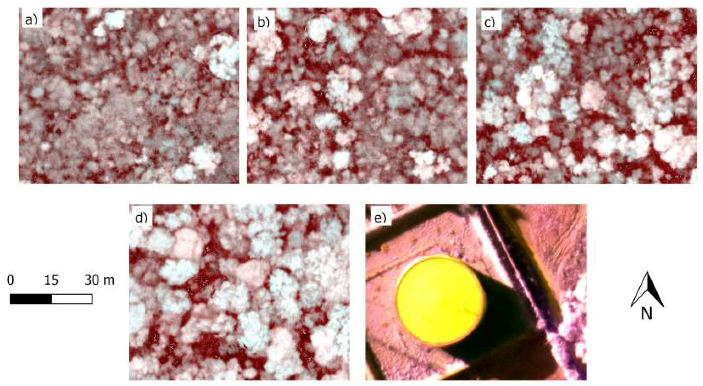
Figure 4.
UAV image view of the four fire-severity strata: very severely burned (a), severely burned (b), burned (c), fully stocked (d), bare land, with buildings (e). Mosaics band composite: NIR-red-green.
Figure 4.
UAV image view of the four fire-severity strata: very severely burned (a), severely burned (b), burned (c), fully stocked (d), bare land, with buildings (e). Mosaics band composite: NIR-red-green.

Figure 5.
Canopy height models with a 0.5 m/pixel resolution, calculated from DTM with a 5 m/pixel resolution (CHM5) (a) and from DTM with a 10 m/pixel resolution (CHM10) (b). Red circle shows the limit of the example plot. CHM profiles (c,d) along the transects marked with a blue line on (a,b). Small differences can be recognised in the results inside the plot area, although, the red arrow on (a) points to a pixelation related to an error on CHM5.

Figure 6.
Canopy height models with a 0.5 m/pixel resolution, calculated from digital terrain model with a 5 m/pixel resolution (CHM5) (a) and from DTM with a 10 m/pixel resolution (CHM10) (b). Blue lines (a,b) show the transects for which CHM profiles are shown in (c,d), respectively. Red rectangles (a,b) represent the areas for which the point cloud profile is shown in (e,f), respectively. The increment of the spacing from 5 m to 10 m for the calculation of DTM allows the selection of low points (more probably related to terrain) from the open canopy areas, reducing the negative effect of obstruction caused by dense canopy cover.

Figure 7.
Scatter plot of ACCI values and BA for each of the 70 plots where both data were available (black dots). The plot shows the thresholds (black dashed line) for defining strata of fire severity based on ACCI values (VSB for very severely burned, SB for severely burned, burned and fully stocked). The red dotted line shows the trend line of an adjusted polynomial equation of second order. The equation and r2 are nor reported, since it is only illustrative: another correlation would be repetitive to the results shown in Table 2.

Figure 8.
Maps of the SPOT6 image classification trained out of BA from the plot-based field inventory (a) and trained out of ACCI from UAV image analysis (b).
Figure 8.
Maps of the SPOT6 image classification trained out of BA from the plot-based field inventory (a) and trained out of ACCI from UAV image analysis (b).

Figure 9.
Box plot of basal area (BA) by forest strata reported separately for the results of the BA-classification (A) and the ACCI-based classification (B). VSB is abbreviation for the stratum ‘very severely burned’, SB for ‘severely burned’. Different letters on top of the whiskers report statistically significant differences between the mean BA among the strata, and white circles report outliers.

Figure 10.
Observed and predicted heights by CHM5 (a,c,e) and CHM10 (b,d,f) of the 71 reference trees (black dots), discriminated by strata (a,b from stratum fully stocked; c,d from stratum burned; e,f from strata SB and VSB). Red lines are trend lines of the adjusted equation, and the blue dotted lines are a reference to the one-to-one ratio.


Table 1.
BA-based and ACCI-based thresholds of fire severity strata.
| Strata | Range of BA (m2/ha) | Range of ACCI Value |
|---|---|---|
| Very severely burned | ≤3.6 | ≤20 |
| Severely burned | >3.6 and ≤6 | >20 and ≤33 |
| Burned | >6 and ≤12 | >33 and ≤66 |
| Fully stocked | >12 | >66 |
Table 2.
Multiple linear regression analysis outputs related to the model shown in Formula (4). The symbol *** means that the inclusion of the dependent variable is significant at a higher percentage of confidence than 99%.
Table 2.
Multiple linear regression analysis outputs related to the model shown in Formula (4). The symbol *** means that the inclusion of the dependent variable is significant at a higher percentage of confidence than 99%.
| Variable | Coefficient | Standard Deviation | t-Value |
|---|---|---|---|
| Intercept | −0.93010 | 0.86051 | 0.284 |
| THC1 | 0.14742 | 0.02998 | 6.26 × 10⁻⁶ *** |
| THC1 | 0.22734 | 0.01810 | <2 × 10-16 *** |
| THC1 | 0.32320 | 0.06330 | 3.09 × 10⁻⁶ *** |
Table 3.
Matrices of predicted and actual strata used for the calculations of the Cohen’s kappa coefficient (k) of both classifications (the ACCI-based and the BA-based classifications).
Table 3.
Matrices of predicted and actual strata used for the calculations of the Cohen’s kappa coefficient (k) of both classifications (the ACCI-based and the BA-based classifications).
| Actual Stratum | |||||||||||
|---|---|---|---|---|---|---|---|---|---|---|---|
| Fully Stocked | Burned | SB | VSB | Total | |||||||
| Predicted stratum | ACCI | BA | ACCI | BA | ACCI | BA | ACCI | BA | ACCI | BA | |
| Fully stocked | 12 | 6 | 3 | 0 | 0 | 0 | 0 | 1 | 15 | 7 | |
| Burned | 5 | 7 | 18 | 24 | 6 | 2 | 2 | 1 | 31 | 34 | |
| SB | 0 | 1 | 6 | 2 | 6 | 9 | 3 | 4 | 15 | 16 | |
| VSB | 0 | 3 | 0 | 1 | 0 | 1 | 15 | 4 | 15 | 9 | |
| Total | 17 | 17 | 27 | 27 | 12 | 12 | 20 | 20 | 76 | 76 | |
Table 4.
Description of the strata based on basal area (BA) (m2/ha). BA-based classification and ACCI-based classification are compared by metrics and errors.
Table 4.
Description of the strata based on basal area (BA) (m2/ha). BA-based classification and ACCI-based classification are compared by metrics and errors.
| Strata | Variable | BA-Based Classification | ACCI-Based Classification |
|---|---|---|---|
| VSB + SB | Area (ha) | 2191.0 | 1850.1 |
| Number of plots | 35 | 30 | |
| Average BA (m2/ha) | 4.3 | 3.2 | |
| Max BA (m2/ha) | 14.4 | 8.9 | |
| Min BA (m2/ha) | 0.0 | 0.0 | |
| Estimation error (m2/ha) | 1.4 | 1.0 | |
| Relative estimation error (%) | 32.14 | 31.22 | |
| Necessary plots to target error | 90 | 73 | |
| Burned | Area (ha) | 1369.4 | 1431.0 |
| Number of plots | 34 | 31 | |
| Average BA (m2/ha) | 10.0 | 8.4 | |
| Max BA (m2/ha) | 31.7 | 14.4 | |
| Min BA (m2/ha) | 3.1 | 3.1 | |
| Estimation error (m2/ha) | 1.8 | 1.1 | |
| Relative estimation error (%) | 18.08 | 13.24 | |
| Necessary plots to target error | 28 | 14 | |
| Fully stocked | Area (ha) | 286.9 | 523.7 |
| Number of plots | 7 | 15 | |
| Average BA (m2/ha) | 15.7 | 16.4 | |
| Max BA (m2/ha) | 21.9 | 31.7 | |
| Min BA (m2/ha) | 3.0 | 9.5 | |
| Estimation error (m2/ha) | 5.6 | 3.2 | |
| Relative estimation error (%) | 35.81 | 19.4 | |
| Necessary plots to target error | 23 | 15 | |
| Bare land | Area (ha) | 96.4 | 139.4 |
Table 5.
Analysis of the strata very severely burned (VSB) and severely burned (SB).
| Strata | Variable | BA-Based Classification | ACCI-Based Classification |
|---|---|---|---|
| VSB | Area (ha) | 1237.6 | 858.0 |
| Number of plots | 19 | 15 | |
| Average BA (m2/ha) | 3.7 | 1.04 | |
| Max BA (m2/ha) | 14.4 | 3.2 | |
| Min BA (m2/ha) | 0.0 | 0.0 | |
| Estimation error (m2/ha) | 2.25 | 0.59 | |
| Relative estimation error (%) | 60.5 | 57.03 | |
| Necessary plots to target error | 174 | 121 | |
| SB | Area (ha) | 953.4 | 992.1 |
| Number of plots | 16 | 15 | |
| Average BA (m2/ha) | 5.0 | 5.4 | |
| Max BA (m2/ha) | 14.0 | 8.9 | |
| Min BA (m2/ha) | 0.8 | 1.9 | |
| Estimation error (m2/ha) | 1.7 | 1.07 | |
| Relative estimation error (%) | 33.27 | 19.85 | |
| Necessary plots to target error | 44 | 15 |
Table 6.
Mean absolute error (MAE) of tree height estimation by CHM5 and CHM10 and coefficient of determination value (from the correlation of observed and estimated tree height), discriminated by fire severity strata. Sample size is reported in parenthesis.
Table 6.
Mean absolute error (MAE) of tree height estimation by CHM5 and CHM10 and coefficient of determination value (from the correlation of observed and estimated tree height), discriminated by fire severity strata. Sample size is reported in parenthesis.
| Strata | Variable | CHM5 | CHM10 |
|---|---|---|---|
| Fully stocked (32) | Mean absolute error (m) | 6.78 | 4.54 |
| RMSE (m) | 8.25 | 5.49 | |
| r2 to observation measurements | 0.06 | 0.12 | |
| Burned (26) | Mean absolute error (m) | 4.02 | 3.39 |
| RMSE (m) | 4.87 | 4.21 | |
| r2 to observation measurements | 0.44 | 0.44 | |
| SB + VSB (13) | Mean absolute error (m) | 2.39 | 2.29 |
| RMSE (m) | 2.96 | 2.85 | |
| r2 to observation measurements | 0.79 | 0.80 |
© 2018 by the authors. Licensee MDPI, Basel, Switzerland. This article is an open access article distributed under the terms and conditions of the Creative Commons Attribution (CC BY) license (http://creativecommons.org/licenses/by/4.0/).
Share and Cite
MDPI and ACS Style
Rossi, F.C.; Fritz, A.; Becker, G. Combining Satellite and UAV Imagery to Delineate Forest Cover and Basal Area after Mixed-Severity Fires. Sustainability 2018, 10, 2227. https://doi.org/10.3390/su10072227
AMA Style
Rossi FC, Fritz A, Becker G. Combining Satellite and UAV Imagery to Delineate Forest Cover and Basal Area after Mixed-Severity Fires. Sustainability. 2018; 10(7):2227. https://doi.org/10.3390/su10072227
Chicago/Turabian StyleRossi, Fernando C., Andreas Fritz, and Gero Becker. 2018. "Combining Satellite and UAV Imagery to Delineate Forest Cover and Basal Area after Mixed-Severity Fires" Sustainability 10, no. 7: 2227. https://doi.org/10.3390/su10072227
Note that from the first issue of 2016, this journal uses article numbers instead of page numbers. See further details here.