Comparison of Forecasting India’s Energy Demand Using an MGM, ARIMA Model, MGM-ARIMA Model, and BP Neural Network Model

Abstract

Better prediction of energy demand is of vital importance for developing countries to develop effective energy strategies to improve energy security, partly because those countries’ energy demands are increasing rapidly. In this work, metabolic grey model (MGM), autoregressive integrated moving average (ARIMA), MGM-ARIMA, and back propagation neural network (BP) are adopted to forecast energy demand in India, the third largest energy consumer in the world after China and the USA. The average relative errors between the actual and simulated value are 1.31% (MGM), 1.07%, 0.92% (MGM-ARIMA), and 0.39% (BP). The high prediction accuracy indicates that the prediction result is effective. The result shows that India’s energy consumption will increase by 4.75% a year in the next 14 years. Compared with the 5.1% per year on average in 1995–2016, India’s energy consumption will still continue its steady growth at about 5% growth from 2017 to 2030.

1. Introduction

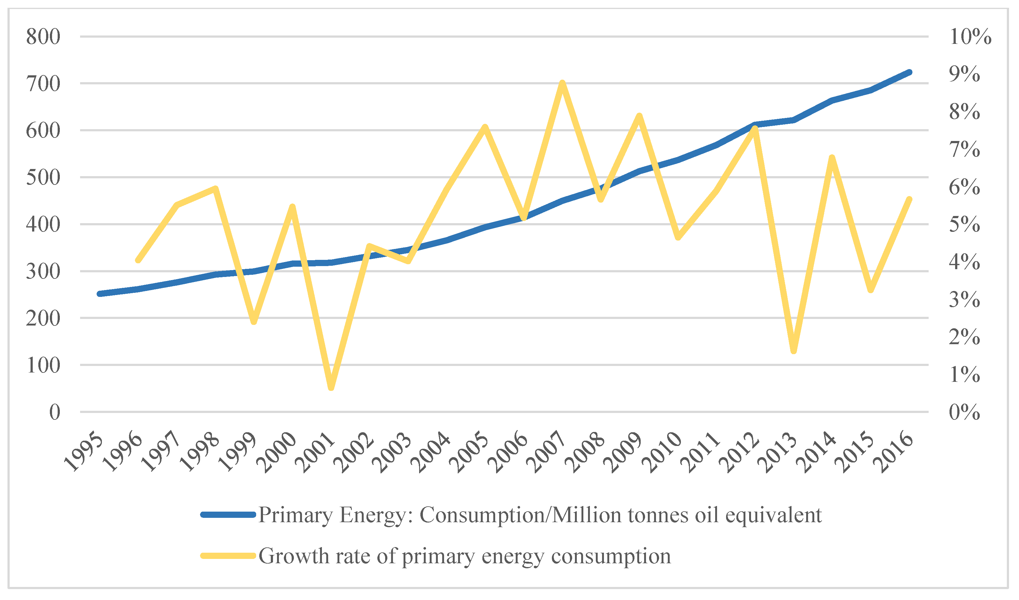
In 2015, the primary energy consumption of India surpassed that of Russia, making India the world’s third-largest energy consumer in 2016. The primary energy consumption of India reached 723.9 million tons oil equivalent, an increase of 129% from 2000, sharing 5% of the world’s primary energy consumption. India’s energy consumption will continue to grow in the future. There are two factors driving the increases in India’s energy consumption: the low per capita energy consumption and the rapid economy growth.

As the world’s second-most populous country, India’s population reached 13.04 billion in 2017, and has continued increasing at an annual rate of 1.4% [1]. The huge population leads to the low per capita energy consumption. According to the research of International Energy Agency, India’s energy consumption per capita is only one-fourth the world average. This means that India’s primary energy demand still has great room for improvement [2]. For example, more and more families will buy their first car with the improvement of living standards, and then the fuel consumption will be increased. In terms of macro economy, India has been in a high growth mode since it started economic reforms in the late 90s [3,4]. In 2015, the growth rate of India’s economy was up to 8% and India surpassed China to become the fastest growing economy in the world [5]. As is shown in the report of the World Bank, India ranked fifth in the world GDP (gross domestic product) in 2016, after the USA, China, Japan, and Germany [6]. In the future, India will need more energy to develop its economy. Also, India will become the dominant driver of the world’s energy demand [7]. Therefore, it is necessary and meaningful to predict the future primary energy consumption of India in this critical period.

For India, the prediction of the primary energy consumption can provide a reference for solving supply and demand contradiction, promoting energy structural supply-side reforms, and creating energy policies. Besides, India’s energy consumption can affect the global energy market directly [8]. Thus, the predictions also offer participants more information, playing an important role in maintaining the market stability. In this paper, we selected India’s primary energy consumption from 1995 to 2016 as our data source, which comes from the BP Statistical Review of World Energy 2017 [9]. We establish four models, metabolic grey model (MGM), autoregressive integrated moving average model (ARIMA), back propagation neural network model (BP), and the combination model of MGM and ARIMA, to forecast India’s primary energy consumption by 2030. The models are based on three theories. The various methods were compared with each other, making the results more persuasive. In this paper, we use mean absolute percentage error (MAPE) and root mean square error (RMSE) to show the results’ reliability.

The structure of this article is as follows: The second section is a literature review. The third section describes the methodology. The fourth section contains the forecasting process and results. The fifth section summarizes the whole paper.

2. Literature Review

In recent years, energy issues have become a top concern of experts and researchers. India is a major energy consumer. In current research, many reviews of energy consumption in different Indian sectors have been made by researchers [10,11,12,13,14,15,16]. Besides, there are many valuable works on energy forecasting. Suganthi et al. forecasted coal, oil, natural gas, and electricity requirements [17]. Ardakani et al. forecasted long-term electrical energy consumption [18]. Mohanty et al. forecasted solar energy with application [19]. Bhattacharya et al. forecasted wood energy [20]. Various models were adopted in these articles. Most of them were simple linear models after improving or combination models based on one theory.

In this area, the grey model, BP neural network model, and ARIMA model are widely used for forecasting of the time series. Compared with the conventional grey model, the improved grey model has a higher forecast accuracy, as it is able to optimize the initial condition and predict both direct and iterative manners [21,22,23,24,25,26]. The nonhomogeneous discrete grey model can better capture nonhomogeneous effects on the data [27]. In addition, GM (grey model) (1,1) by month-flame optimization with a rolling mechanism made the timeliness of the data series more clear [28,29].

Sen et al. used ARIMA to forecast the energy consumption of an Indian pig iron manufacturing organization, the results of which appeared smoother than the seasonal random trend model [10]. The ARIMA model has been improved greatly. Temporal aggregation could achieve a better estimation of the different time series components, and the forecasting combination could reduce the importance of the model selection [30]. The ARIMA model could meet the subject’s characteristics of self-similarity, periodicity, suddenness, and trends, delivering better forecasting performance in short-term forecasting [31]. So, this model has been applied broadly throughout other critical industries, such as public transport, metal prices, and the assessment of health care structures [32,33,34,35,36,37,38,39].

BP network is a feed forward neural network realized by a back propagation algorithm [21]. It a non-linear prediction model, achieving a stable prediction effect through determining the combining weights [40,41]. Researchers improved the network based on particle swarm optimization and an optimized genetic algorithm to make it ideal for many application scenarios [42,43,44]. Currently it is already used in energy forecasting, and the error is less than 2% [18].

Therefore, the time sequence prediction method has been widely used in in various fields. It has been already generally accepted in academia. However, recent research has mostly been based on one theory, where the conflicts between the results of different methods can be avoided and the precision is also difficult to ensure. Without comparison, it is hard to find the models with higher accuracy. In addition, compared with a single model, forecasting with multiple models gives greater superiority in the precision of results [29,45,46,47].

In this paper, we used the MGM, ARIMA model, MGM-ARIMA model, and BP neural network model to forecast India’s energy demand. The models were established according to three theories: the grey theory, regression analysis theory, and neural network theory. The first two methods are linear, while the last is nonlinear. This method system solves the limitations of former researches where the time sequence prediction method is applied, and further improves the prediction accuracy. The use of three theories enriches the theoretical foundation of forecasting in our work. We hope to provide a methodological reference for analogous study.

We applied this method system to forecasting India’s energy demand. As the world’s third-largest energy consumer, India’s energy demand can affect not only its own development but also the world energy market’s changes. Thus, the forecasting results will provide data referencing for the Indian government’s creation of energy policies, and offer participants more information about the world energy market.

3. Methodology

The research object of this paper is the energy demand of India. The forecasting work for this dataset includes the following two characteristics: the energy consumption forecasts rely only on historical data, that is to say, this dataset belongs to univariate prediction; and the energy consumption in the next 12 years is the ultimate forecast target, indicating that a model with advantages in long-term forecasting needs to be chosen. In addition, as is stated in the literature review, the MGM, ARIMA model, and BP neural network have high accuracy in forecasting. Moreover, combination approaches covering both linear and nonlinear models further improve the accuracy. So, the MGM, ARIMA model, MGM-ARIMA model, and BP neural network model are suitable for this study.

In this section, we introduce the principles of the four models. For ease of understanding, we use detailed formulas to explain their operation. The meaning of the symbols in equations is given in

Table 1. Explanation of the symbols in formulas.

Notations	Explanation	Notations	Explanation
$x^{\left(0\right)}\left(\mathrm{k}\right)$	Original sequence	$Y_t^{\ast }$	Predicted data sequence
$x^{\left(1\right)}\left(\mathrm{k}\right)$	Once accumulated sequence	‘d’	Order of the difference
${\widehat{x}}^{\left(0\right)}\left(k\right)$	Prediction of raw sequence	‘p’	Order of auto-regression
${\widehat{x}}^{\left(1\right)}\left(k\right)$	Prediction of 1-AGO sequence	‘q’	Order of moving average
t	Time sequence	$E_t$	Initial residual sequence
B	Matrix of data and constants	$E_t^{\ast }$	Predicted residual sequence
$Y_N$	Matrix of data	K	Sample number
‘α’ ‘μ’	Constant parameter	n	Nodes’ number
‘c’	Constant term	i	Hidden layer’ number
${\alpha }_i$, ${\beta }_i$	Harmonic parameter	$E_p$	Error sequence
${\mu }_t$	Error term of early data	$t_{pi}$	Expected output sequence
$Y_t$	Initial data sequence	$o_{pi}$	Actual output sequence

.

3.1. Metablic Gey Model (1,1)

The MGM (1,1) is a widely used forecasting model. Its essence is to use the time series itself to predict future data under the condition that time series shows a clear trend.

The original sequence is recorded:

$$X^{\left(0\right)}=\left(x^{\left(0\right)}\left(1\right),x^{\left(0\right)}\left(2\right),\dots ,x^{\left(0\right)}\left(\mathrm{n}\right)\right)$$

(1)

In order to make the sequence change regularly, we employ the accumulation tool. After accumulating, the once accumulated sequence (1-AGO) is obtained: ${\mathrm{X}}^{\left(1\right)}=\left\{{\mathrm{x}}^{\left(1\right)}\left(1\right),{\mathrm{x}}^{\left(1\right)}\left(2\right),\dots ,{\mathrm{x}}^{\left(1\right)}\left(\mathrm{n}\right)\right\}\mathrm{f}$, where $x^{\left(1\right)}\left(k\right)={\sum }_{i=1}^k{x}^{\left(0\right)}\left(i\right), k=1,2,3,\dots ,n$. So, if we obtain the accumulated sequence, the value of the predicted data sequence can be also obtained by subtraction.

$${\widehat{x}}^{\left(0\right)}\left(k+1\right)={\widehat{x}}^{\left(1\right)}\left(k+1\right)-{\widehat{x}}^{\left(1\right)}\left(k\right)=\left(1-e^{\alpha }\right)\left(x^{\left(0\right)}\left(1\right)-\frac{\mu }{\alpha }\right)e^{-\alpha k}, k=1,2,\cdots ,n$$

(2)

Through much experimenting, the first-order accumulated series meets a linear first-order differential equation.

$$\frac{d{x}^{\left(1\right)}}{dt}+\alpha x^{\left(1\right)}=\mu$$

(3)

After derivation, the relationship between the sequences ${\widehat{x}}^{\left(1\right)}\left(k\right)$ and $x^{\left(0\right)}\left(\mathrm{k}\right)$ can be described by the following formula:

$${\widehat{x}}^{\left(1\right)}\left(k\right)=\left(x^{\left(0\right)}\left(1\right)-\frac{\mu }{\alpha }\right)e^{-\alpha \left(k-1\right)}+\frac{\mu }{\alpha },k=1,2,\cdots ,n$$

(4)

In Equation (4), we can acquire the solution as long as the parameters ‘$\mathsf{\alpha }$’ and ‘μ’ are known. ‘$\mathsf{\alpha }$’ and ‘μ’ can be solved by the least squares method.

$${[\mathsf{\alpha },\mathsf{\mu }]}^{\mathrm{T}}={\left({\mathrm{B}}^{\mathrm{T}}\mathrm{B}\right)}^{-1}{\mathrm{B}}^{\mathrm{T}}{\mathrm{Y}}_{\mathrm{N}}$$

(5)

$${\mathrm{Y}}_{\mathrm{N}}={\left[{\mathrm{x}}^{\left(0\right)}\left(2\right),\dots ,{\mathrm{x}}^{\left(0\right)}\left(\mathrm{n}\right)\right]}^{\mathrm{T}}$$

(6)

$$\mathrm{B}=\left[\begin{array}{c}\begin{array}{cc}-{\mathrm{Z}}^{\left(1\right)}\left(2\right)& 1\\ -{\mathrm{Z}}^{\left(1\right)}\left(3\right)& 1\end{array}\\ \begin{array}{cc}⋮& ⋮\\ -{\mathrm{Z}}^{\left(1\right)}\left(\mathrm{n}\right)& 1\end{array}\end{array}\right]$$

(7)

In Equation (7), $Z^{\left(1\right)}\left(k\right)=0.5x^{\left(1\right)}\left(k\right)+0.5x^{\left(1\right)}\left(k-1\right), k=2,3,\cdots ,\mathrm{n}.$

Lastly, we substitute the values of ‘$\mathsf{\alpha }$’ and ‘μ’ into Equation (4), so the sequence ${\widehat{x}}^{\left(1\right)}\left(k\right)$ can be solved, and then by calculating Equation (2), the prediction data can be also obtained.

3.2. Autoregressive Integrated Moving Average Model (ARIMA)

ARIMA is short for autoregressive integrated moving average model. It is the combination of the differenced autoregressive model and moving average model, with a high accuracy of prediction. The modeling is divided into two steps.

The first step involves computing the difference of a non-stationary sequence. We need use the formula below to make the original sequence $Y_t$ stationary. After d order difference, we obtain the new stationary sequence $Y_t^{\ast }$.

$$Y_t^{\ast }={\left(1-B\right)}^d{Y}_t$$

(8)

In Equation (8), $B=\left(\begin{array}{cc}-\left(y_1^1+y_2^1\right)/2& 1\\ ⋮& ⋮\\ -\left(y_{m-1}^1+y_m^1\right)/2& 1\end{array}\right)$.

The second step involves moving average processes and autoregressive processes.

$$Y_t^{\ast }=\mathrm{c}+{\alpha }_1{Y}_{t-1}+{\alpha }_2{Y}_{t-2}+\cdots +{\alpha }_p{Y}_{t-p}+u_t$$

(9)

$$Y_t^{\ast }=u_t+{\beta }_1{u}_{t-1}+{\beta }_2{u}_{t-2}+\cdots +{\beta }_q{u}_{t-q}$$

(10)

Therefore, the complete formula for the ARIMA model is:

$$Y_t^{\ast }=\mathrm{c}+{\alpha }_1{Y}_{t-1}+{\alpha }_2{Y}_{t-2}+\cdots +{\alpha }_k{Y}_{t-k}+{\mu }_t+{\beta }_1{\mu }_{t-1}+{\beta }_2{\mu }_{t-2}+\cdots +{\beta }_q{\mu }_{t-q}$$

(11)

where p denotes the order of auto-regression and q is the order of the moving average. They can be determined with the autocorrelation coefficient map and partial autocorrelation coefficient map, respectively. ‘${\alpha }_k$’ and ‘${\beta }_k$’ are regression coefficients.

3.3. MGM-ARIMA Model

This model is the combination of MGM and ARIMA. Therefore, it involves two parts.

The first part involves predicting the original data spanning from 1995 to 2016 by using an MGM (1,1) model. With cumulative series and a linear first-order differential equation, we can obtain the predicted series. The theory was discussed in Section 3.1. After prediction, the error between the predictive value and original value can be easily obtained.

$${\mathrm{E}}^{\left(0\right)}={\left[{\mathrm{e}}^{\left(0\right)}\left(1\right),{\mathrm{e}}^{\left(0\right)}\left(2\right)\dots ,{\mathrm{e}}^{\left(0\right)}\left(\mathrm{n}\right)\right]}^{\mathrm{T}}$$

(12)

$${\mathrm{e}}^{\left(0\right)}\left(\mathrm{i}\right)={\hat{\mathrm{x}}}^{\left(0\right)}\left(\mathrm{i}\right)-{\mathrm{x}}^{\left(0\right)}\left(\mathrm{i}\right)$$

(13)

where x indicates the original series and $\hat{\mathrm{x}}$ denotes the predicted series.

The second part involves predicting the error using the ARIMA model. At first, the difference of a non-stationary error sequence is computed. After that, we obtain the new stationary error sequence.

$$E_t^{\ast }={\left(1-B\right)}^d{E}_t$$

(14)

We then take the moving average step and autoregressive step.

$$E_t^{\ast }=\mathrm{c}+{\alpha }_1{E}_{t-1}+{\alpha }_2{E}_{t-2}+\cdots +{\alpha }_p{E}_{t-p}+u_t$$

(15)

$$E_t^{\ast }=u_t+{\beta }_1{u}_{t-1}+{\beta }_2{u}_{t-2}+\cdots +{\beta }_q{u}_{t-q}$$

(16)

The complete formula for the ARIMA model is:

$$E_t^{\ast }=\mathrm{c}+{\alpha }_1{E}_{t-1}+{\alpha }_2{E}_{t-2}+\cdots +{\alpha }_k{E}_{t-k}+{\mu }_t+{\beta }_1{\mu }_{t-1}+{\beta }_2{\mu }_{t-2}+\cdots +{\beta }_q{\mu }_{t-q}$$

(17)

where $E_t$ stands for the original error sequence;$E_t^{\ast }$ represents the new stationary error sequence; p is the order of auto-regression; and q is the order of the moving average.

3.4. BP Neural Network Model

BP neural network is the most successful neural network in prediction fields. It consists of an input layer, output layer, and a few hidden layers. There are a certain number of nodes on each layer and one node represents one neuron. The number can be determined by this empirical formula:

$${\sum }_{i=0}^n{C}_{n_i}^i>K$$

(18)

where K is the sample number; $n_i$ is the number of the hidden layer’s node; n is the number of the input layer’s node; and $C_{ni}^i$ = 0 if i > n.

In the network, the upper nodes connect the lower nodes by the weight matrix. The nodes’ connection between layers is full, but on one layer there is no connection. The ordinary transfer function is the Sigmoid function.

$$f\left(x\right)=\frac{1}{1+e^{-x}}$$

(19)

There are two singles flows between layers: working information and error. The working signal is from the input layer. It is the function of input data and the weight matrix. The error signal is from the output layer. It is the difference between the true output and expected output, and the error $E_p$ can be calculated using Equation (20):

$$E_p=\frac{1}{2}\ast \sum {\left(t_{pi}-o_{pi}\right)}^2$$

(20)

In the above formula, $t_{pi}$ denotes the expected output and $o_{pi}$ represents the true output.

During the process of propagation, the weight matrix of the network are constantly adjusted. The structure is as shown in Figure 1. Finally, when the aim of the actual output being consistent with the expected output is achieved, then the network can be used for prediction directly.

4. Empirical Results

This paper selected a set of data spanning from 1995 to 2016 obtained from the BP Statistical Review of World Energy 2017 (as shown in Figure 2). In the period of 1995–2016, India’s primary energy consumption showed an upward trend, and the growth rate was about 5.1% per year on average.

4.1. MGM (1,1) Model Parameters

The first step is to define an original sequence $X^{\left(0\right)}=\left(x^{\left(0\right)}\left(1\right),x^{\left(0\right)}\left(2\right),\dots ,x^{\left(0\right)}\left(22\right)\right)$, where $x^{\left(0\right)}\left(1\right)$ represents India’s primary energy consumption in 1995.

The second step involves the sequence accumulation, $X^{\left(1\right)}=\left(x^{\left(1\right)}\left(1\right),x^1\left(2\right),\dots ,x^{\left(1\right)}\left(22\right)\right)$, and subsequently the establishment of the linear first-order differential equation. We can solve the parameters ‘α’ and ‘μ’ using the least squares method, which is shown in

Table 2. The value of the metabolic grey model’s (MGM) parameters in 2000–2030.

	2000	2001	2002	2003	2004	2005	2006	2007	2008	2009	2010
α	−0.05	−0.04	−0.03	−0.03	−0.03	−0.05	−0.06	−0.06	−0.07	−0.07	−0.07
μ	245.89	260.29	280.11	287.79	298.27	295.13	301.04	314.42	330.00	355.20	374.02
	2011	2012	2013	2014	2015	2016	2017	2018	2019	2020	2021
α	−0.06	−0.06	−0.06	−0.05	−0.05	−0.04	−0.05	−0.05	−0.05	−0.05	−0.05
μ	411.85	439.52	466.25	502.03	533.57	570.89	580.05	615.70	638.43	674.30	706.32
	2022	2023	2024	2025	2026	2027	2028	2029	2030
α	−0.05	−0.05	−0.05	−0.05	−0.05	−0.05	−0.05	−0.05	−0.05
μ	739.23	777.23	813.92	853.64	895.30	938.45	984.05	1031.6	1081.0

.

The third step is to obtain the fitted value (1995–2016) and the predicted value (2017–2030) with EXCEL. As is shown in Figure 3, the fitted value of the MGM is very close to the original value; however, there is a difference for the year 2013. The reason for this is that India’s primary energy consumption in 1995–2016 showed a rising trend, but it slowed down suddenly in 2013, as illustrated in Figure 2. We regard this abrupt variation as a non-linear characteristic. Yet, as a linear forecasting model, the MGM is applicable to the case where the growth rate of the original data series is relatively stable. If the original data series is characterized by nonlinear characteristics, the fitting effect of the MGM will degrade. Thus, the fitted value of the MGM is very close to the original value, except in 2013. In the following section of our article, we use other models to overcome these loopholes to obtain a better fitting effect.

4.2. ARIMA Model Parameters

The condition of the ARIMA time series model is that random sequence is stationary. In order to smooth the sequence, we performed differential processing for the sequence by using the unit root test. The unit root test and difference results are shown in

Table 3. Unit root test and difference results based on Eviews 7.2.

Sequence	ADF Statistic	Critical Value			Value of p
		1%	5%	10%
Q	−2.961334	−4.571559	−3.690814	−3.286909	0.1685
Q*	−2.437015	−4.616209	−3.710482	−3.297799	0.3502
Q**	−5.767150	−4.571559	−3.690814	−3.286909	0.0011

Note: Q means zero-order difference; Q* means first-order difference; Q** means second-order difference.

.

As illustrated in Table 3, the second-order difference is stable. Then, obtained with the help of EViews 7.2, our correlation coefficient graph for a stationary sequence is shown in Figure 4.

According to the coefficient judgment criteria of the ARIMA model, ARIMA (2,2,1) can be used to predict the future consumption. Then we need to determine the goodness of fit for the model. With the help of SPSS software, we determined that $R^2$ is 0.809 > 0.60, which means that the fitting effect is good (

Table 4. Parameters of the goodness of fit for the autoregressive integrated moving average (ARIMA) (2,2,1) model.

Model	Number of Predictions	Model Fit Statistics		Number of Outliers
		Stationary R-Squared	R-Squared
ARIMA (2,2,1)	1	0.809	0.809	0

).

Finally, the fitted result achieved by the ARIMA model is shown in Figure 5. Obviously, the fitting effect is good, but there is still a difference for the year 2013. The reason for this is that the ARIMA model is also a linear model, and it cannot deal with nonlinear characteristics. This situation will be improved in the combination model and nonlinear model.

4.3. MGM-ARIMA Model Parameters

In this model, the first step is to obtain the absolute error. So, we used the consumption fitted by the MGM from 1995 to 2016. The original data and fitting results are shown in

Table 5. Initial fitted result based on the MGM (1,1) model.

Year	Primary Energy Consumption/Million Tons of Equivalent	Initial Prediction	Absolute Error
1995	251.5716	251.5716	0.0000
1996	263.4000	261.7342	1.6658
1997	275.7442	276.1579	−0.4137
1998	288.6670	292.5813	−3.9143
1999	302.1954	299.6023	2.5931
2000	316.3578	315.9773	0.3805
2001	329.0027	318.0086	10.9941
2002	330.2666	332.0359	−1.7693
2003	341.8766	345.3628	−3.4862
2004	354.3913	365.8556	11.4643
2005	381.5452	393.6102	12.0650
2006	413.9138	413.9578	−0.0440
2007	441.6681	450.2354	−8.5673
2008	479.0618	475.7145	3.3473
2009	508.6667	513.2210	−4.5543
2010	549.7625	537.0707	12.6918
2011	572.7613	568.6912	4.0701
2012	603.5870	611.6017	−8.0147
2013	644.7245	621.4868	23.2377
2014	661.6280	663.5853	−1.9573
2015	693.5195	685.0938	8.4257
2016	713.8711	723.9023	10.0312

. The last column is the absolute error.

The second step is to predict the error using the ARIMA. Obviously, this sequence is not stationary. So, we performed differential processing for the sequence using the unit root test. The result in

Table 6. Unit root test and difference results based on Eviews 7.2.

Sequence	DF Statistic	Critical Value			Value of p
		1%	5%	10%
Q	−5.007479	−4.467895	−3.644963	−3.261452	0.0034
Q*	−9.463064	−4.498307	−3.658446	−3.268973	0.0000
Q**	−3.833027	−4.667883	−3.733200	−3.310349	0.0422

Note: Q means zero-order difference; Q* means first-order difference; Q** means second-order difference.

shows that the second-order difference is stable.

As illustrated in Table 6, the second-order difference is stable. Then, we drew a correlation coefficient graph for a stationary sequence (shown in Figure 6).

For the third step, based on the analysis above, we decided to use the ARIMA (2,2,1) model to predict the future error from 1995 to 2030. Then, we used SPSS software to determine the goodness of fit for the model. The result in

Table 7. Parameters of goodness of fit for the ARIMA (2,2,1) model.

Model	Number of Predictions	Model Fit Statistics		Number of Outliers
		Stationary R-Squared	R-Squared
ARIMA (2,2,1)	1	0.834	0.834	0

shows that $R^2$ is 0.834 > 0.60, which means that the fitting effect is good.

Through the relations among the original consumption, the MGM (1,1) prediction consumption, and the ARIMA prediction error, we can obtain the prediction consumption. The fitting curve is shown in Figure 7. The excellent fitting effect can be seen intuitively.

4.4. BP Neural Network Model Parameters

MATLAB is an internationally recognized, outstanding mathematical application software. In particular, its neural network box offers facilities for BP network modeling. Therefore, we used MATLAB to establish the BP neural network and predict data. The process involves three steps.

The first step is to establish a BP neural network. We used the special function ‘newff’ to determine the numbers of layers, the number of nodes, and the transfer function, such as the following: ‘net = newff ([−1,1],[4,4,1])’. After establishing the network, we needed to set these values.

The second step is the network initialization. The number of nodes on the input layer and output layer was 1,1. After many debugging repetitions, the number of nodes on each of the hidden layers was set to 4, 4, 1. The structure of the network is shown in Figure 8. In order to meet the accuracy requirements, the permissible error is set to 0.00000001. The training iteration is 1000.

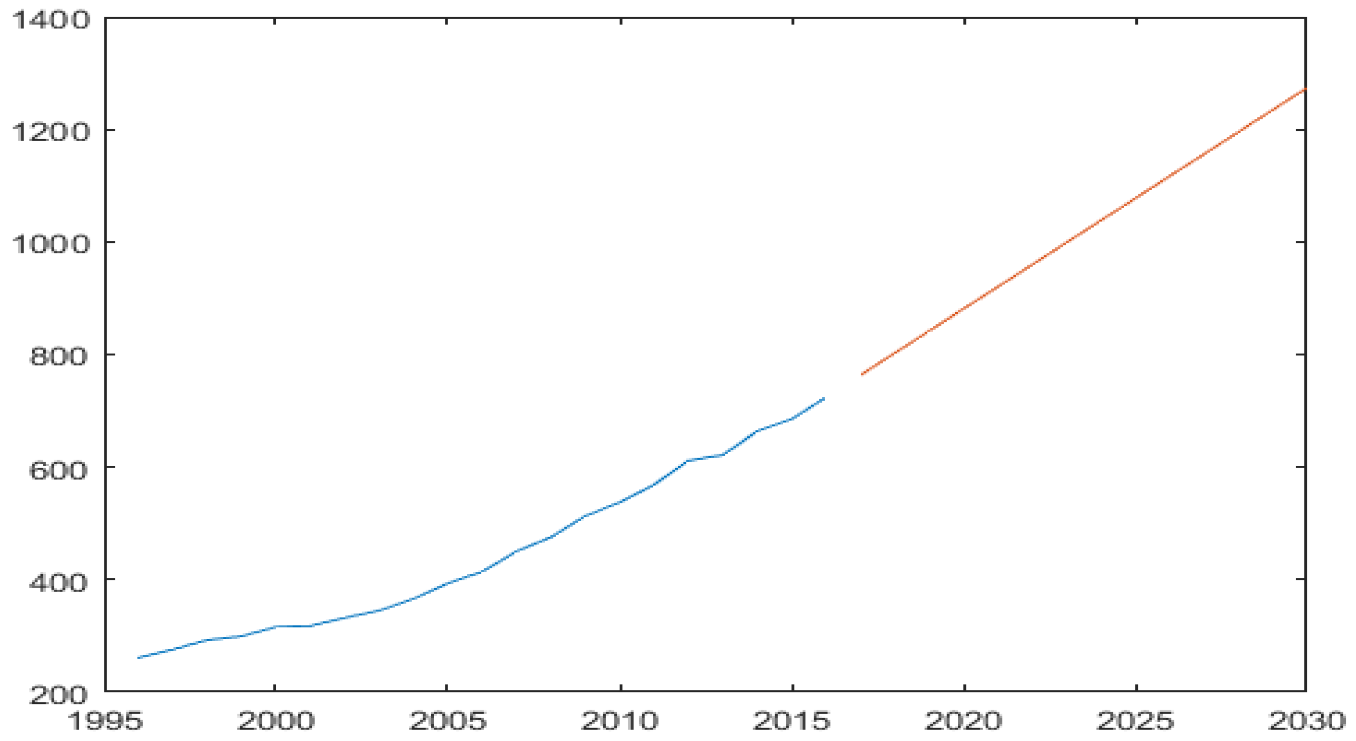
The third step is the network training simulation. We used the function ‘sim’ to achieve this. Y = sim(net,p), where y indicates the output data, net denotes the object of the neural network, and p represents the input vectors. The consumptions from 1995 to 2013 were selected as the training sample, and the consumptions from 2014 to 2016 as the test sample. The predicted curve generated by MATLAB is shown in Figure 9.

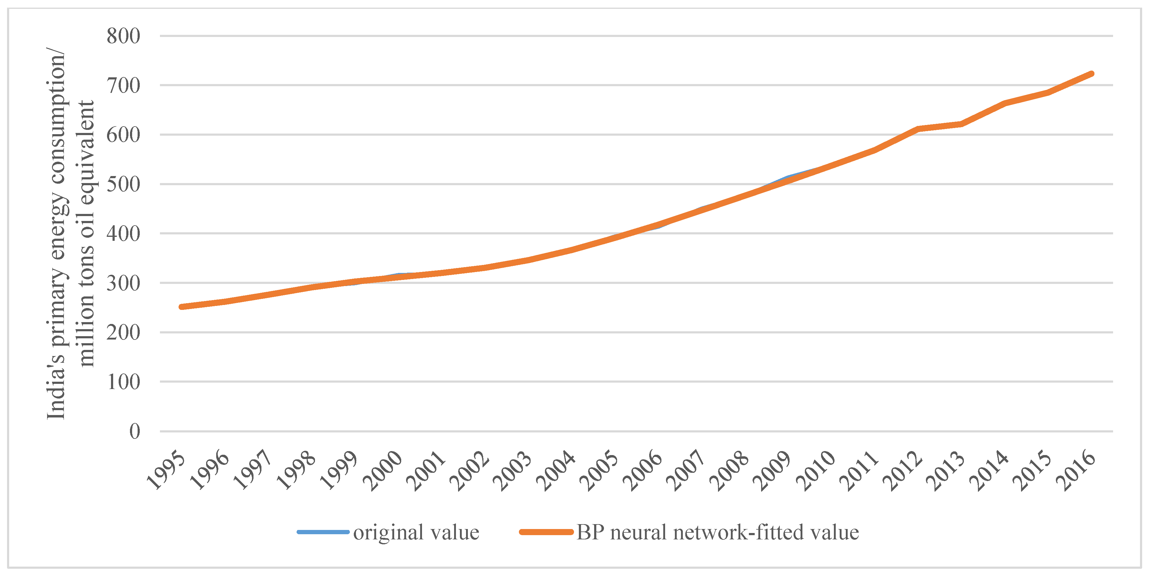
It is clear that the fitted value generated by the BP neural network is very close to the actual value from 1995 to 2016, as shown in Figure 10. The fitting curve almost coincides with the original data curve.

4.5. Comparison and Evaluation of Multiple Models

From Figure 3, Figure 5, Figure 7, and Figure 10, we can see that the fitting effect was very good. However, in order to accurately judge the error, we calculated the MAPE (mean absolute percentage error) and RMSE (root mean square error) of the four models based on the following formulas. The result of the error calculation is shown in

Table 8. MAPE and RMSE of the four models (%).

	MGM (1,1)	ARIMA	MGM-ARIMA	BP Neural Network
MAPE	0.0131	0.0107	0.0092	0.0039
RMSE	8.2599	6.1846	5.3811	2.3224

.

$$\mathrm{MAPE}=\frac{|y_i-x_i|}{x_i}$$

$$\mathrm{RMSE}=\sqrt{\frac{\sum {\left(y_i-x_i\right)}^2}{n}}$$

According to the above analysis, the accuracy of all of the four models is high. From Figure 11, we can see that the average accuracy of the four models is all more than 95%. The higher prediction accuracy indicates that the prediction results are persuasive. As expected, compared with a single model, the combination model (MGM-ARIMA) has higher accuracy. However, the forecasting result of the BP neural network model is the most reliable of all models.

4.6. Forecast Results

Based on the primary energy consumption of India from 1995 to 2016 obtained from the BP Statistical Review of World Energy 2017,

Table 9. Forecasting results of the four models.

	MGM (1,1)	ARIMA	MGM-ARIMA	BP Neural Network
2017	759.33	764.83	761.35	763.16
2018	793.41	792.26	804.99	802.43
2019	834.72	846.97	847.37	841.71
2020	873.93	874.52	893.09	880.99
2021	916.30	929.61	940.48	920.27
2022	961.20	970.22	992.38	959.55
2023	1007.01	1017.07	1045.59	998.83
2024	1055.93	1074.22	1103.12	1038.10
2025	1106.76	1115.79	1163.49	1077.40
2026	1159.49	1182.11	1226.89	1116.70
2027	1215.41	1229.01	1294.59	1156.00
2028	1273.02	1294.20	1365.19	1195.20
2029	1333.86	1354.93	1440.26	1234.50
2030	1396.97	1415.01	1518.90	1273.80

shows the concrete results of the final forecast of the four models. The prediction results (shown in Figure 12) indicate that India’s primary energy consumption will increase continually at a rate of 4.75% over the next 14 years.

5. Conclusions

In this paper, we established four models (the MGM, ARIMA model, MGM-ARIMA model, and BP neural network model) to forecast India’s energy demand. As shown in Figure 11, all four models have high accuracy above 95%. Unlike those in past research, our models are based on three theories, which overcomes the limitations that the conflicts between the results are ignored, precision is difficult to ensure, and it is hard to find a better model without comparison. The comparison of multiple models’ precision indicates that the combination model (MGM-ARIMA) has higher accuracy than a single model (MGM and ARIMA), and the BP neural network is the most reliable among all models.

The extraordinary precision indicates that the prediction results are persuasive. The forecasting results show that India’s primary energy consumption will grow at a rate of about 4.75% over the next 14 years. Compared with the rate of 5.1% per year on average for 1995–2016, India’s energy consumption will continue its steady growth at about a 5% growth from 2017 to 2030. This trend is consistent with our evaluation. In the future, with the increase of the primary energy demand, energy problems and climate change will be increasingly prominent. The Indian government and other national governments should make efforts to control both the supply and demand of energy. Suggested concrete measures are as follows:

(i)

For India itself, government decision-makers should secure the energy supply from the long-term benefits. The Indian government should take vigorous action to develop some new and renewable energy sources such as wind energy, hydro energy, solar energy, terrestrial heat, biomass energy, etc.

(ii)

For the world market, India’s increasing energy demand is an assault. Participating nations should increase communication to promote the development of new energy together. Only by diversifying the energy mix can the energy supply fundamentally be secured.

(iii)

Curtailing energy demand is also vital. India should vigorously conserve energy in various sectors, popularize energy-conserving technology and equipment, and improve energy efficiency. For example, adjusting energy prices can cut down consumption to some degree.

In addition, the highest precision of the BP neural network implies that the research still leaves something to be desired. In this paper, we employed the time vector as the only input parameter. However, the BP neural network has more value in the research of a complicated system affected by various factors. Though the forecasting result using one factor has high accuracy already, its superiority is not fully realized. Therefore, the BP neural network’s application to energy forecasting needs further exploration.

References

- The World Bank. World Band Data—India; The World Bank: Washington, DC, USA, 2017. [Google Scholar]
- IEA. The World Energy Outlook 2016; The International Energy Agency: Paris, France, 2016. [Google Scholar]
- Kapoor, R. India @ 2050: The future of the Indian economy. Futures 2014, 56, 1–7. [Google Scholar] [CrossRef]
- Wang, Q.; Li, R. Drivers for energy consumption: A comparative analysis of China and India. Renew. Sustain. Energy Rev. 2016, 62, 954–962. [Google Scholar] [CrossRef]
- Broadberry, S.; Custodis, J.; Gupta, B. India and the great divergence: An Anglo-Indian comparison of GDP per capita, 1600–1871. Explor. Econ. Hist. 2015, 55, 58–75. [Google Scholar] [CrossRef] [Green Version]
- The World Bank. Wrold Band Indicator—Economy; The World Bank: Washington, DC, USA, 2017. [Google Scholar]
- Kalyani, K.A.; Pandey, K.K. Waste to energy status in India: A short review. Renew. Sustain. Energy Rev. 2014, 31, 113–120. [Google Scholar] [CrossRef]
- Shahbaz, M.; Mallick, H.; Mahalik, M.K.; Sadorsky, P. The role of globalization on the recent evolution of energy demand in India: Implications for sustainable development. Energy Econ. 2016, 55, 52–68. [Google Scholar] [CrossRef] [Green Version]
- BP. BP Statistical Review of World Energy 2017; BP: London, UK, 2017. [Google Scholar]
- Sen, P.; Roy, M.; Pal, P. Application of ARIMA for forecasting energy consumption and GHG emission: A case study of an Indian pig iron manufacturing organization. Energy 2016, 116, 1031–1038. [Google Scholar] [CrossRef]
- Wang, Q.; Jiang, R.; Li, R. Decoupling analysis of economic growth from water use in City: A case study of Beijing, Shanghai, and Guangzhou of China. Sustain. Cities Soc. 2018, 41, 86–94. [Google Scholar] [CrossRef]
- Nejat, P.; Jomehzadeh, F.; Taheri, M.M.; Gohari, M.; Majid, M.Z.A. A global review of energy consumption, CO2 emissions and policy in the residential sector (with an overview of the top ten CO2 emitting countries). Renew. Sustain. Energy Rev. 2015, 43, 843–862. [Google Scholar] [CrossRef]
- Franco, S.; Mandla, V.R.; Rao, K.R.M. Urbanization, energy consumption and emissions in the Indian context A review. Renew. Sustain. Energy Rev. 2017, 71, 898–907. [Google Scholar] [CrossRef]
- Gupta, C.L.; Rao, K.U.; Vasudevaraju, V.A. Domestic energy consumption in India (Pondicherry region). Energy 1980, 5, 1213–1222. [Google Scholar] [CrossRef]
- Tripathi, L.; Mishra, A.K.; Dubey, A.K.; Tripathi, C.B.; Baredar, P. Renewable energy: An overview on its contribution in current energy scenario of India. Renew. Sustain. Energy Rev. 2016, 60, 226–233. [Google Scholar] [CrossRef]
- Wang, Q.; Li, R. Journey to burning half of global coal: Trajectory and drivers of China’s coal use. Renew. Sustain. Energy Rev. 2016, 58, 341–346. [Google Scholar] [CrossRef]
- Suganthi, L.; Samuel, A.A. Modelling and forecasting energy consumption in INDIA: Influence of socioeconomic variables. Energy Sources Part B Econ. Plan. Policy 2016, 11, 404–411. [Google Scholar] [CrossRef]
- Ardakani, F.J.; Ardehali, M.M. Long-term electrical energy consumption forecasting for developing and developed economies based on different optimized models and historical data types. Energy 2014, 65, 452–461. [Google Scholar] [CrossRef]
- Mohanty, S.; Patra, P.K.; Sahoo, S.S.; Mohanty, A. Forecasting of solar energy with application for a growing economy like India: Survey and implication. Renew. Sustain. Energy Rev. 2017, 78, 539–553. [Google Scholar] [CrossRef]
- Bhattacharya, S.C. Wood energy in India: Status and prospects. Energy 2015, 85, 310–316. [Google Scholar] [CrossRef]
- Chen, G.; Fu, K.; Liang, Z.; Sema, T.; Li, C.; Tontiwachwuthikul, P.; Idem, R. The genetic algorithm based back propagation neural network for MMP prediction in CO2-EOR process. Fuel 2014, 126, 202–212. [Google Scholar] [CrossRef]
- Geng, N.; Yong, Z.; Sun, Y.X.; Jiang, Y.J.; Chen, D.D. Forecasting China’s annual biofuel production using an improved grey model. Energies 2015, 8, 12080–12099. [Google Scholar] [CrossRef]
- Xiong, P.P.; Dang, Y.G.; Yao, T.X.; Wang, Z.X. Optimal modeling and forecasting of the energy consumption and production in China. Energy 2014, 77, 623–634. [Google Scholar] [CrossRef]
- Hamzacebi, C.; Es, H.A. Forecasting the annual electricity consumption of Turkey using an optimized grey model. Energy 2014, 70, 165–171. [Google Scholar] [CrossRef]
- Wang, Q.; Chen, X. Energy policies for managing China’s carbon emission. Renew. Sustain. Energy Rev. 2015, 50, 470–479. [Google Scholar] [CrossRef]
- Wang, Q.; Li, R. Decline in China’s coal consumption: An evidence of peak coal or a temporary blip? Energy Policy 2017, 108, 696–701. [Google Scholar] [CrossRef]
- Ayvaz, B.; Kusakci, A.O. Electricity consumption forecasting for Turkey with nonhomogeneous discrete grey model. Energy Sources Part B Econ. Plan. Policy 2017, 12, 260–267. [Google Scholar] [CrossRef]
- Zhao, H.; Zhao, H.; Guo, S. Using GM (1, 1) Optimized by MFO with Rolling Mechanism to Forecast the Electricity Consumption of Inner Mongolia. Appl. Sci. 2016, 6, 20. [Google Scholar] [CrossRef]
- Li, S.; Yang, X.; Li, R. Forecasting China’s Coal Power Installed Capacity: A Comparison of MGM, ARIMA, GM-ARIMA, and NMGM Models. Sustainability 2018, 10, 506. [Google Scholar] [CrossRef]
- Kourentzes, N.; Petropoulos, F.; Trapero, J.R. Improving forecasting by estimating time series structural components across multiple frequencies. Int. J. Forecast. 2014, 30, 291–302. [Google Scholar] [CrossRef] [Green Version]
- Cui, Z.; Li, L.; Zhao, C.; Yang, T. Traffic Analysis and Forecasting of Power Video Services Based on ARIMA Model. J. Tianjin Univ. 2015, 48, 49–55. [Google Scholar]
- Ediger, V.Ş.; Akar, S. ARIMA forecasting of primary energy demand by fuel in Turkey. Energy Policy 2007, 35, 1701–1708. [Google Scholar] [CrossRef]
- Onasanya, O.K.; Olakunle, O.A.; Emmanuel, A.O. Forecast Performance of Multiplicative Seasonal Arima Model: An Application to Naira/Us Dollar Exchange Rate. Am. Statist. 2014, 101, 1566–1581. [Google Scholar]
- Oliveira, E.M.D.; Oliveira, F.L.C. Forecasting mid-long term electric energy consumption through bagging ARIMA and exponential smoothing methods. Energy 2018, 144, 776–788. [Google Scholar] [CrossRef]
- Akpinar, M.; Yumusak, N. Year Ahead Demand Forecast of City Natural Gas Using Seasonal Time Series Methods. Energies 2016, 9, 727. [Google Scholar] [CrossRef]
- Tsai, C.H.; Mulley, C.; Clifton, G. Forecasting public transport demand for the Sydney greater metropolitan area: A comparison of univariate and multivariate methods. Road Transp. Res. 2014, 23, 51. [Google Scholar]
- Kriechbaumer, T.; Angus, A.; Parsons, D.; Casado, M.R. An improved wavelet–ARIMA approach for forecasting metal prices. Resour. Policy 2014, 39, 32–41. [Google Scholar] [CrossRef] [Green Version]
- Muriana, C.; Piazza, T.; Vizzini, G. An expert system for financial performance assessment of health care structures based on fuzzy sets and KPIs. Knowl. Based Syst. 2016, 97, 1–10. [Google Scholar] [CrossRef]
- Wang, Q.; Jiang, X.-T.; Li, R. Comparative decoupling analysis of energy-related carbon emission from electric output of electricity sector in Shandong Province, China. Energy 2017, 127, 78–88. [Google Scholar] [CrossRef]
- Liu, Y.K.; Xie, F.; Xie, C.L.; Peng, M.J.; Wu, G.H.; Xia, H. Prediction of time series of NPP operating parameters using dynamic model based on BP neural network. Ann. Nucl. Energy 2015, 85, 566–575. [Google Scholar] [CrossRef]
- Adhikari, R. A neural network based linear ensemble framework for time series forecasting. Neurocomputing 2015, 157, 231–242. [Google Scholar] [CrossRef]
- Ren, C.; An, N.; Wang, J.; Li, L.; Hu, B.; Shang, D. Optimal parameters selection for BP neural network based on particle swarm optimization: A case study of wind speed forecasting. Knowl. Based Syst. 2014, 56, 226–239. [Google Scholar] [CrossRef]
- Yu, F.; Xu, X. A short-term load forecasting model of natural gas based on optimized genetic algorithm and improved BP neural network. Appl. Energy 2014, 134, 102–113. [Google Scholar] [CrossRef]
- Wang, Q.; Li, R. Natural gas from shale formation: A research profile. Renew. Sustain. Energy Rev. 2016, 57, 1–6. [Google Scholar] [CrossRef]
- Yuan, C.; Liu, S.; Fang, Z. Comparison of China’s primary energy consumption forecasting by using ARIMA (the autoregressive integrated moving average) model and GM(1, 1) model. Energy 2016, 100, 384–390. [Google Scholar] [CrossRef]
- Li, S.; Li, R. Comparison of forecasting energy consumption in Shandong, China Using the ARIMA model, GM model, and ARIMA-GM model. Sustainability 2017, 9, 1181. [Google Scholar]
- Barak, S.; Sadegh, S.S. Forecasting energy consumption using ensemble ARIMA–ANFIS hybrid algorithm. Int. J. Electr. Power Energy Syst. 2016, 82, 92–104. [Google Scholar] [CrossRef]
Figure 1.
The structure of the back propagation (BP) neural network.
Figure 2.
India’s primary energy consumption and growth rate in 1995–2016.
Figure 3.
Gap between actual and MGM (1,1) prediction values.
Figure 4.
Autocorrelation and partial autocorrelation coefficients.
Figure 5.
Gap between actual and ARIMA prediction values.
Figure 6.
Figure 7.
Gap between actual and MGM-ARIMA prediction values.
Figure 8.
Structure of the BP neural network.
Figure 9.
Predicted curve generated by MATLAB.
Figure 10.
Gap between actual and BP neural network prediction values.
Figure 11.
The fitting goodness value of multiple models at different time points.
Figure 12.
India’s primary energy consumption forecasted by the four models.