Temporal Stability of Groundwater Depth in the Contemporary Yellow River Delta, Eastern China


1
College of Resources and Environment, Shandong Agricultural University, Tai’an 271018, China
2
National Engineering Laboratory for Efficient Utilization of Soil and Fertilizer Resources, Tai’an 271018, China
3
Centre for Real Estate, Royal Agricultural University, Cirencester GL7 6JS, UK
*
Authors to whom correspondence should be addressed.
Sustainability 2018, 10(7), 2224; https://doi.org/10.3390/su10072224
Submission received: 10 May 2018
/
Revised: 11 June 2018
/
Accepted: 20 June 2018
/
Published: 28 June 2018
(This article belongs to the Special Issue Sustainable Use of Soils and Water: the Role of Environmental Land Use Conflicts)
Abstract
:Sustainable development calls for the wise use of groundwater resources. Of particular concern is saline intrusion into productive agricultural land, which is contiguous with densely populated coastal settlements. To reverse saline intrusion in such coastal regions, information about the groundwater depth in terms of its spatio-temporal variability is essential. Using survey data from 2004 to 2007, the research revealed the temporal variation characteristics of groundwater depth in the Contemporary Yellow River Delta. It explored the temporal stability characteristics of groundwater depth by using the coefficient of variation, Spearman rank correlation coefficient, and average relative deviation and standard deviation, and confirmed that the representative point reflected the average groundwater depth of the study area. Results showed that spatial variation of the groundwater depth in the study area was medium, but the variation coefficient of groundwater depth showed the seasonal changes. The spatial variation coefficient was largest in the dry season; the other months were relatively stable. The groundwater depth in the study area had strong temporal stability. The correlation between the Spearman rank correlation coefficient and the time lags showed that the spatial pattern of groundwater depth in the study area was similar across two or three years but the similarity weakened beyond this period. The representative points of the whole area showed a good linear correlation, and were spatially concentrated. In different years or time periods, the representative points were not the same but belonged to the medium groundwater depth grade in the area. The study provides useful guidance for Yellow River irrigation, preventing saline intrusion and the restoration of saline-alkali soils. It offers a theoretical basis for identifying regional satellite groundwater depth monitoring points.
1. Introduction
Over the past couple of decades, China has undergone spectacular economic development, coupled with deteriorating environmental conditions [1]. From 1998 to 2012, the proportion of urban population increased from 30.4% to 52.6% but the urbanization and industrialization process consumed 7.93 million ha of farmland [2]. Aware of the danger, China is restructuring its growth towards quality. Specifically, to mitigate the pressure of farmland loss and guarantee national food security, the Chinese government has recently adopted a series of farmland exploitation policies.
The Yellow River Delta (YRD) is one of China’s three major river delta systems. Geologically, it is relatively young land that was formed less than 150 million years ago. Its name reflects the 1 billion tons of sediment the Yellow River carries annually downstream into its estuary where the deposits increase land area by about 2400 hm2 annually [3]. Engineering-focused national policy has sought to exploit the rich land resources of the YRD. For example, the YRD is the core demonstration area in the “Bohai granary project” that is known as the National Science and Technology Support Program. However, as a newly formed estuarine delta, YRD is naturally characterized by extensive coverage of primary salinization [4]. Over recent decades, secondary anthropogenic salinization has also been severe to the extent that it now threatens food production and the environment [5,6]. For these reasons, the Chinese central government plans to restore salinized land in the YRD and especially control secondary salinization. The YRD is dominated by rivers and oceans, so groundwater is shallow. Indeed, in most areas it is less than 3 m below the surface but has a high degree of salinity. These characteristics of groundwater, coupled with silt soil texture, lead to a strong soil capillary effect which brings groundwater salt to the soil surface. Therefore, in this region the salt transportation characteristics of groundwater is especially important with soil salinity strongly linked to groundwater depth (GD) [7,8]. For national food security and to sustainably exploit the YRD agricultural potential without saline intrusion, information on GD is urgently needed. However, GD is highly and nonlinearly variable in both time and space due to the heterogeneity of surface water, topography, seawater intrusion and human activities such as irrigation and drainage. Eltahir and Yeh demonstrated that seasonal variations of shallow groundwater are strongly influenced by climatologic variables, including precipitation and evapotranspiration [9]. Many authors, including Famiglietti et al., Brocca et al., and Li and Rodell, have investigated soil moisture spatio-temporal variability [10,11,12]. Western and Blöschl found it increased with increasing extent [13]. However, the study of GD spatio-temporal variability often requires a large amount of observation data and many monitoring points. Unfortunately, in most areas, observation wells are generally sparse. Therefore, few studies have been conducted on GD spatio-temporal variability owing to the scarcity of available, high-quality measurement time series at a regional scale. Satellite-based remote sensing methods can provide time series of GD estimates over large areas. For instance, at regional scales the Gravity Recovery and Climate Experiment (GRACE) satellite observations have proved useful for evaluating groundwater variations and trends [14,15], but the GRACE spatial resolution is about 15,000 km2 at mid-latitudes [16,17], making it difficult to validate remote sensing data with well observations. The economic use of remote sensing to accurately estimate average GD for large areas calls for data validation. The first step to solve this validation problem is to identify representative groundwater monitoring points.
Temporal stability is the most important feature of soil property spatio-temporal variability. This concept was first described by Vachaud et al. who defined it as “the time-invariant association between spatial location and classical statistical parameters of a given soil property’’ [18]. The concept was later expanded by Kachanoski et al., who described the temporal stability of soil property as a reflection of the temporal persistence of the spatial structure. Temporal stability indicates the degree by which soil moisture content spatial patterns change over time; a strong temporal stability indicates a stable pattern over time even though the actual soil moisture content values may vary greatly within a given area [19]. Temporal stability analysis has been successfully applied to identify locations that represent the mean soil moisture content of an area [20]. Soil moisture content information can be up-scaled or downscaled and even resolve missing data sets [21,22,23]. GD temporal stability assessment helps resolve GD issues but also improves the design of groundwater monitoring networks. Knowledge of temporal variability helps determine the number of wells required to quantify the regional mean GD at a given time. Despite its importance in helping to identify stable spatio-temporal variability structures to control soil salinization, no GD study has been conducted.
The study had four main objectives: (1) to clarify the spatial pattern and the temporal stability characteristics of GD in the Contemporary Yellow River Delta; (2) to identify temporally stable locations to reduce time series sampling of average GD on a regional scale (approximately 3000 km2); (3) to determine how long temporal stability can persist; and (4) to identify time-stable points for effective remote sensing data validation. To illustrate the benefits of the time-stability concept, the research compared the average GD determined from time-stable points with GD data from satellite remote sensing.
The research articulated optimization of a well observation network and illuminated how validated satellite data could be employed cost-effectively to monitor GD.
2. Materials and Methods
2.1. Study Area
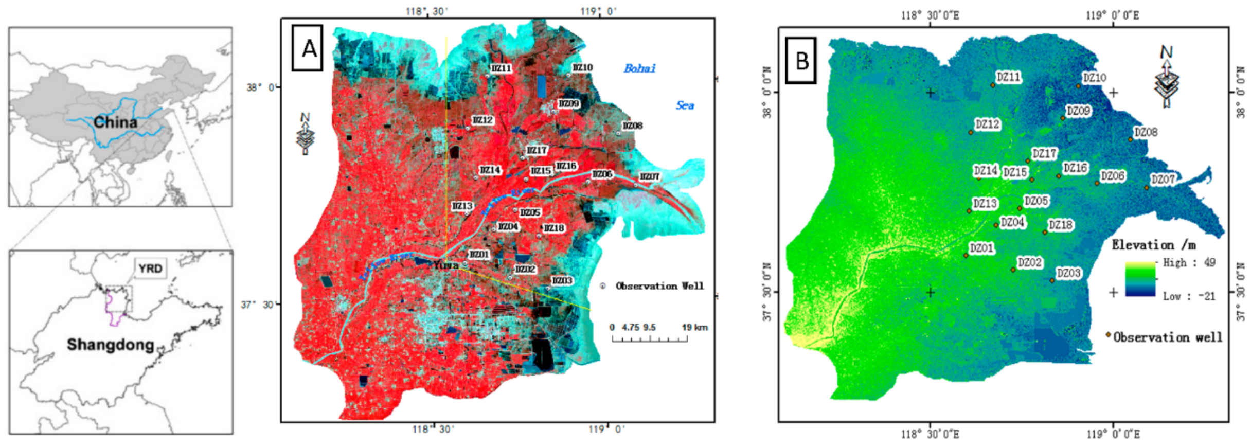
The Yellow River Delta (117°31′–119°18′ E, 36°55′–38°16′ N) is situated in the northeast of the Shandong Province, China, on the southern bank of the Bohai Sea (Figure 1). The YRD is traversed by the Yellow River, which conveys heavy sediment discharge. The nutrient-rich waters support a classical river wetland ecosystem which sustains the most important population of migrating birds in the world. The YRD is composed by the ancient, modern and contemporary delta body. The contemporary delta is a fan shape resulting from a periodic swing of the mouth channel, with the Yuwa village as the vertex. Since 1934, the delta has grown to reach its current 3000 km2 (Figure 1). In Figure 2, the yellow line displays the boundary of the contemporary delta. The study area was in the contemporary delta but sampling points (Figure 1) were limited to by the availability of observation wells which restricts interpolation of the results. The climate is characterized by continental monsoon in the North Temperate Zone with seasonal fluctuations in precipitation and temperature. The annual average precipitation and evaporation are approximately 600 mm and 1944 mm, respectively, with 70% of the total precipitation occurring between July and August [24]. Currently, large-scale irrigation system construction to introduce Yellow River water into reservoirs and channels proceeds apace with ongoing intensification of land use.
2.2. Data and Method
2.2.1. Data Collection
(1) Groundwater depth dataset
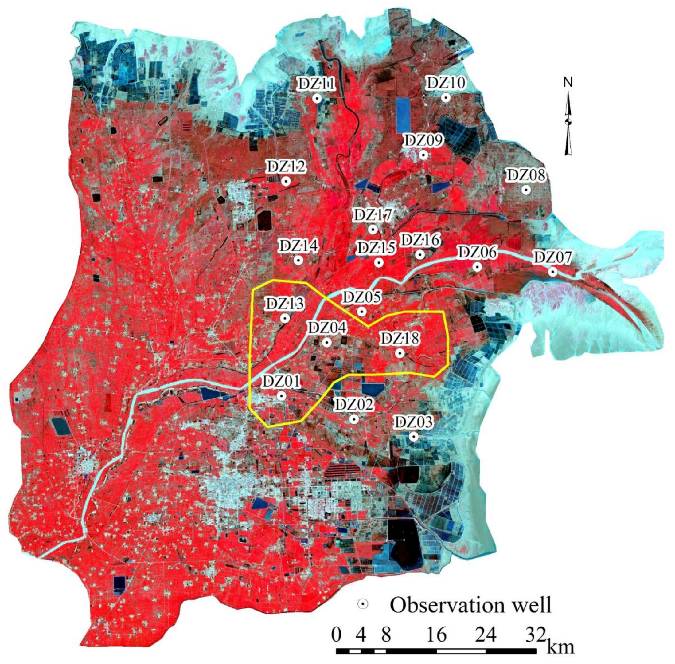
The GD dataset came mainly from 18 observation wells numbered DZ01 to DZ18, measured at regular intervals during the period of 2004–2007. Generally, the depth of the observation well was 5–6 m, with well tube diameter 50 mm. The material of well wall is PVC, and the lower part of the wall tube consists of some small holes, surrounded by a fine sand and other filter media. The groundwater monitoring device has a probe for detecting the GD and conductivity (see Figure 1). The location of observation wells was determined based on the accessibility of roads and the gradient of the GD, as shown in Figure 1. In the study area, groundwater monitoring wells DZ01, DZ04, DZ05, DZ06, DZ07, DZ13, DZ15 and DZ16 were arranged from inland to the coast, but also close to the Yellow River channel.DZ02, DZ03, DZ18, DZ14, DZ17, DZ08, DZ09, DZ12, DZ10, and DZ11 are distributed from south to north.
Measurements began on 5 May 2004. Initially, researchers measured only the ten wells located to the north of the Yellow River. On the following day, wells south of the Yellow River were measured. From then on, each point was measured once every 5 days, and all locations were sampled each time in the same time and order.
Researchers took three measurements and the truncated mean was computed by discarding the highest and the lowest value. Researchers also measured the geography coordinates and elevation data of the wells by GPS device. Researchers logged measurement time, irrigation, precipitation and other weather conditions in situ.
(2) Elevation data
We used the elevation data from the processed SRTM (Shuttle Radar Topography Mission) DATA VERSION 4.1. The data are in Geotiff format with 90 m resolution, in decimal degrees and datum WGS84. They are derived from the USGS/NASA SRTM-4 data (http://srtm.csi.cgiar.org); the elevation map of the study area is shown as Figure 1B.
(3) Terrestrial water storage (TWS) dataset
In this study, we used the Level-3 products from the GRACE project data products as the TWS. The Level-3 mass anomalies datasets are associated with the most up-to-date Level-2 data obtained from three data centers: Jet Propulsion Laboratory (JPL), Center for Space Research (CSR), and Geo Forschungs Zentrum Potsdam (GFZ). Monthly mean TWS equivalent thickness, 1° × 1° gridded data files were retrieved from the GRACE Tellus website (https://grace.jpl.nasa.gov/data/get-data/monthly-massgrids-land/), CU GRACE website (http://geoid.colorado.edu/grace/dataportal.html) and ICGEM website (http://icgem.gfz-potsdam.de/ICGEM/ICGEM.html).
(4) Surface water and soil moisture storage dataset
Surface water (SW) and soil moisture storage (SMS) were obtained from the outputs of the Community Land Model 2.0 (CLM 2.0) in Global Land Data Assimilation System (GLDAS-1) Products corresponding to the study period. Outputs of CLM are available since 1979 at the spatial resolution of 1 degree, and the study area only has one grid cell. The monthly SMS was computed by aggregating SMS of all the soil layers with a total soil thickness ranging from 0 cm to 82.9 cm.
2.2.2. Method of Deriving Maps of the Groundwater Depth
We calculated the groundwater tables for the wells by subtracting the GD from the elevation measured in situ. Then, a digital groundwater table model (DGTM) was produced by using Inverse Distance Weight (IDW) interpolation. In discontinuous environments with weak soil moisture spatial correlation, linear regression models can capture the impact of features and outperform distance-based methods. Nevertheless, in complex terrains such as the YRD, IDW outperforms Kriging for interpolation. The resolution of the DGTM data was the same as the SRTM data, and the maps of the mean GD for each month were derived by subtracting the DGTM from the elevation data.
2.2.3. Satellite-Based Groundwater Storage Anomaly Estimation
To determine the anomaly in satellite-based groundwater storage (DGWS), anomalies of other water components of terrestrial water cycle, i.e., soil moisture (DSM), snow water equivalent (DSNW) and surface water (DSW) equivalents, were removed from terrestrial water storage (TWS). Correspondingly, monthly SMS changes were computed as the difference of SMS in two consecutive months. The spatial averages of monthly evapotranspiration and SMS changes were computed from 1980 to 2015. The monthly evapotranspiration (E) and changes in SMS (DSMS) were aggregated to obtain annual values.
2.2.4. Method of Analysis: Temporal Stability
To characterize the GD temporal stability, the research estimated standard soil moisture statistics.
Coefficient of Variation
The coefficient of variation captured the spatial variability of GD. The coefficient of variation ( reflects the relative variability at sampling times; in other words, the degree of discretization of the random variable and is defined as:
where: σ is the GD standard deviation in a given sampling time, μ is the average GD at sampling time.
In order to characterize the degree of variability, the coefficient of variation () values were analyzed as suggested by Nielsen and Bouma [25], can quantitatively ascertain the magnitude of the spatial variability as weak when < 10%, moderate if 10% < < 100% and strong when > 100%.
Relative Deviation
The temporal stability of the GD patterns was also assessed following the classic approach of the ranking stability analysis [18,19,22]. This encompassed the computation of the mean relative difference (MRD) and standard deviation of relative difference (SDRD) for all measurements. The relative difference was defined as:
where is the GD measured at site i and time j.
Represents the mean value of GD at time j, and n is the number of sampling sites. Therefore, the mean relative difference for site i was defined as:
where m represents the number of sampling times. Similarly, the standard deviation of the relative difference at site i was defined as:
The mean relative deviation and its standard deviation reflect the temporal stability of the GD. The smaller the relative deviation and the standard deviation, the higher the temporal stability. Therefore, the principle of “when the average relative deviation is close to zero, the standard deviation is small” was employed to select the well locations on behalf of the averaged conditions.
Spearman Rank Correlation Coefficient
The Spearman rank correlation coefficient method is a non-parametric test method which can express the intensity and direction of the same variable at different times. In this study, we used this statistic to compare the similarity and persistence for the GD spatial pattern on different dates by means of autocorrelation analysis. The Spearman rank correlation coefficient was defined as:
where Rij is the rank of GD measured at site i and time j, Rik is the rank of the GD measured at site i but at time k, and n is the total number of observations. A Spearman rs equal to 1 indicates a total agreement of the spatial patterns between the two dates and therefore perfect temporal stability of the GD. In other words, the closer is to one, the more stable the process involved. Spearman rank correlation coefficient was computed for each study site.
The statistical analyses and plots of the GD data used SPSS 16.0 and Excel 2013 software.
3. Results and Analysis
3.1. Group the Observation Wells
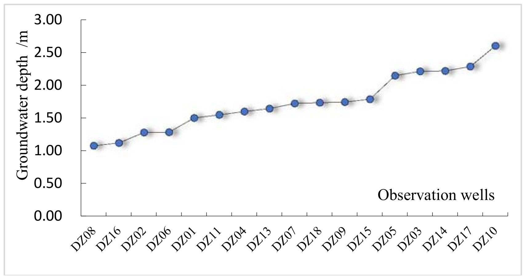
Figure 2 illustrates the observation wells, sorted according to the average of the GD during the study period.
As can be seen from Figure 2, the GD average in the area is high, roughly between 1.0 m and 3.0 m. the maximum and the minimum value of the mean GD in the study area appeared at DZ10 and DZ08 in Figure 2 respectively. Based on the curvature typology of the GD in Figure 2, the observation wells can be divided into three groups: wells with lower GD including DZ05 DZ03, DZ14, DZ17 and DZ10, wells with higher GD including DZ08, DZ16. DZ02 and DZ06, others are wells with medium GD.
3.2. Temporal Dynamics of Groundwater Depth
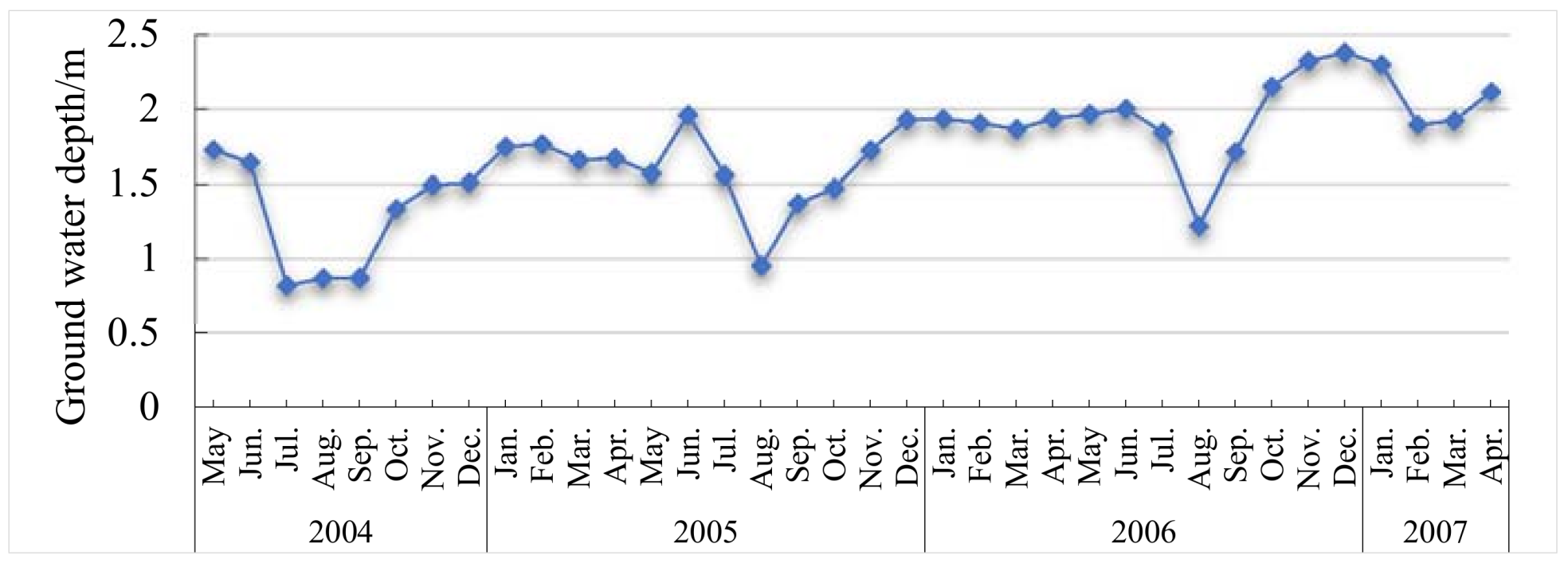
The statistical characteristics of the GD obtained from the monthly average of all the observation wells in the period from 2004 to 2007 are shown in Figure 3.
From Figure 3, the GD in the Contemporary Yellow River Delta has obvious monthly variation, and the GD varied in response to precipitation and surface water in this area. A sharp decrease in GD occurred and reached the minimum value in months 7–9 each year which corresponds to the wet period and rainy season. After the rains, precipitation and water level decrease as the Yellow River enters its local dry season. Notwithstanding seasonal fluctuations, in general groundwater depth gradually increases to its maximum between December and February which corresponds to the usual regional dry season. Regional droughts in spring 2005 and 2006 explain the spike and sustained high GD reflecting the low water level.
3.3. Spatial Variation Characteristics over Time
The spatial variance of each month in the study area was calculated according to Equation (1), and the results are shown in Figure 4.
Figure 4 shows that the monthly variation coefficient of GD in the study area fluctuated between 24.96% and 73.04% during the study period. According to the grouping rules described above for the degree of spatial variance in Equation (1), the degree of GD spatial variation is moderate in the Contemporary YRD.
The fluctuation of the spatial variation of GD illustrated distinct seasonal cycles. Generally, peaks in variation coefficient manifested in July–September 2004, July–August 2005 and August 2006, respectively. These periods corresponded to the wet season in the study area where groundwater was at shallow depth. In comparison, the fluctuation of the spatial variance in other months was gentle. In addition, the spatial variance showed a decreasing trend from 2004 to 2007, which is consistent with the characteristic for the temporal dynamics of the GD.
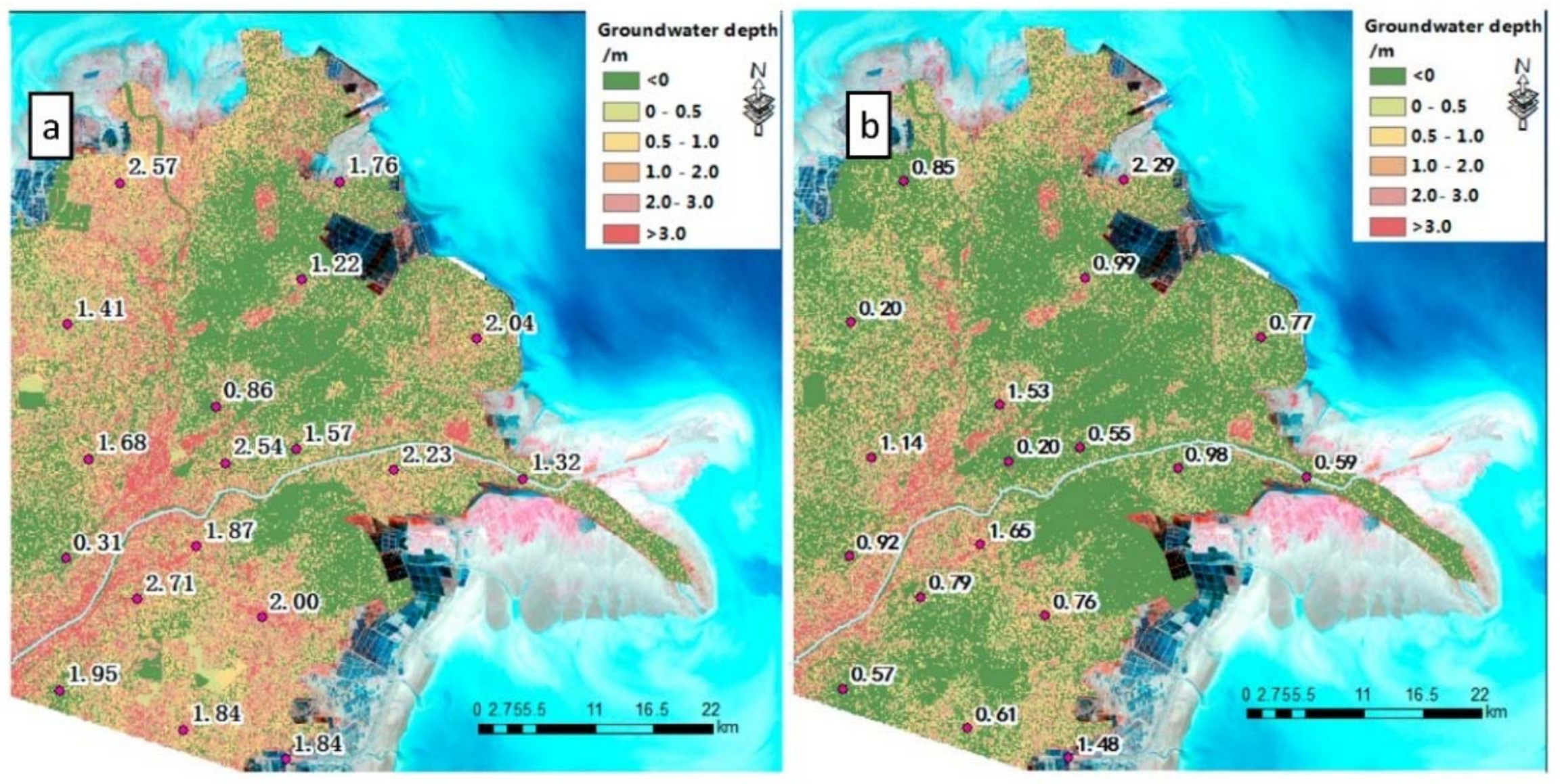
We visually demonstrated the spatial variance features of the GD and compared the possible switch in the spatial organization of GD with the season change. Taking 2005 as an example, interpolated maps of the GD were created for both wet periods and dry periods in the study area by the method listed in Section 2.2.2. The maps are presented in Figure 5.
The resulting maps (Figure 5a,b), despite a certain degree of uncertainty for some border areas due to extrapolation, confirm and make the spatial patterns during the two conditions visually appreciable. On the maps, the places where the buried depth is less than zero were covered with surface water. Figure 6 illustrates that, overall, the spatial distribution of GD in August was more dispersed and staggered in different grades than in January, indicating the spatial variance was more distinct in the wet period than other months during a season cycle.
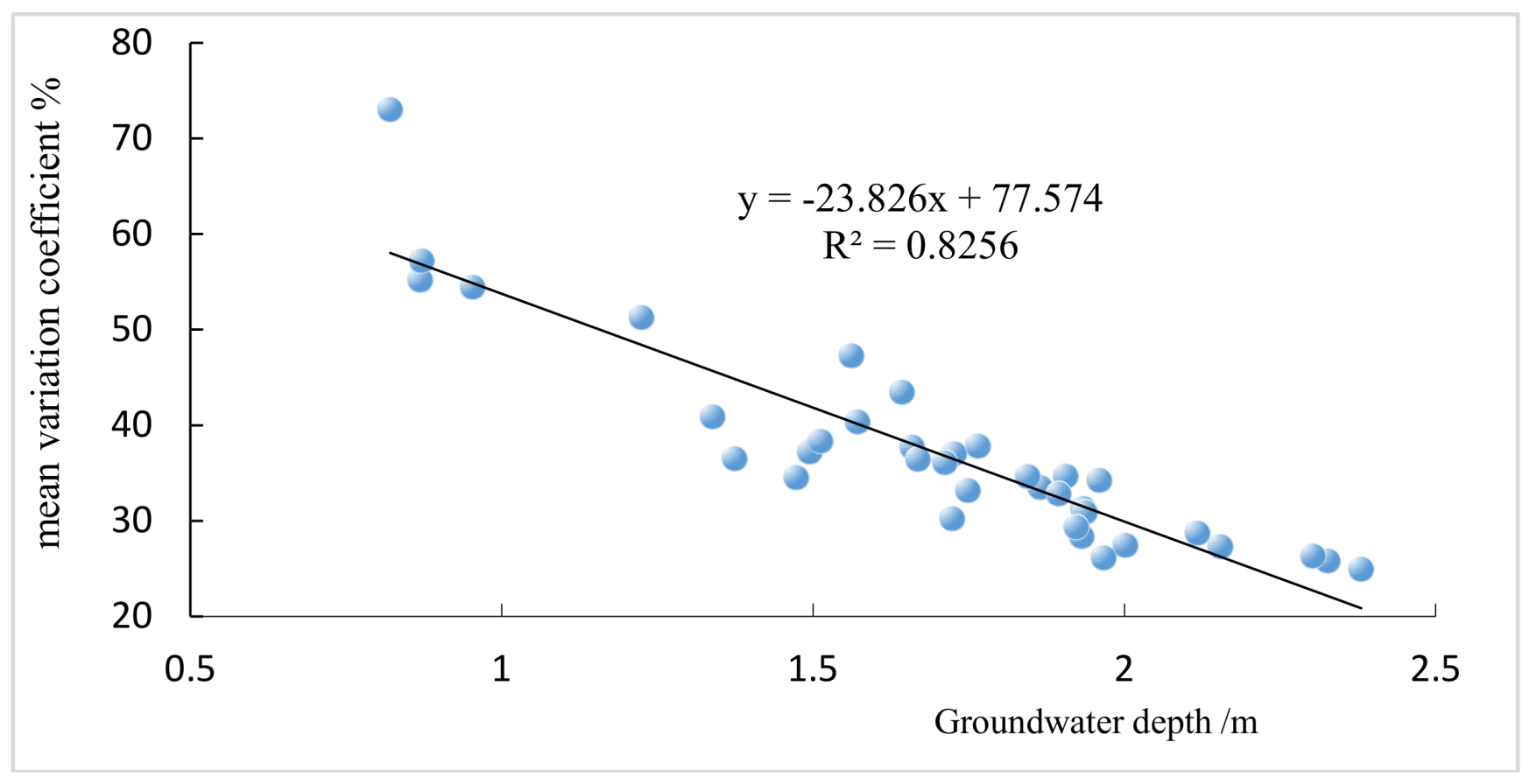
Furthermore, to make clear the relationship between spatial variability and GD, statistical regression analysis was performed on the monthly mean GD across the whole region and monthly spatial variation coefficients, as shown in Figure 6.
Figure 6 illustrates that the spatial variance coefficient has a good linear negative correlation with the GD, with the coefficient R2 of the model being 0.83, which indicates that when the groundwater of the whole study area is higher, the regional spatial variation is larger. According to the meteorological data of the study region, in 2006, a dry year, the GD was lower than in 2004 and 2005, and the mean annual GD in these three years was 1.43 m, 1.68 m and 1.99 m with corresponding spatial variability coefficients of 43.98%, 36.39% and 30.93% respectively. The serial data of annual averages validates the relevance between the two variances, but also implies that, in this region, climate plays a more significant role in influencing the spatial variability of GD. The research confirmed spatial variability of groundwater depth: compared to wet periods, drought weakens it.
3.4. Time Stability of Groundwater Depth
3.4.1. Analysis for the Temporal Stability of Spatial Pattern
Spearman’s rank correlation coefficients confirmed the temporal stability for spatial patterns of GD. The results for past months are presented in Table 1. The scatter plot of the mean GD and the Spearman rank correlation coefficient for each month is shown in Figure 7.
The values in Table 1 show that the relationships were significant at p < 0.01 or p < 0.05 in most months, indicating strong time persistence in the spatial pattern of GD across the study area. These results are consistent with those in other areas [18,26,27,28,29]. Figure 8 shows that the Spearman rank correlation coefficient is lower at the observation wells when the monthly mean GD >2 m or <1 m (labeled with red circles) while, when the groundwater is in medium depth, the Spearman rank correlation coefficients are higher, implying the spatial patterns of GD in these months are similar to that of other times. These results indicate that the temporal stability for spatial patterns of GD is seasonal, in dry or wet season, it is poor, while in regular season it is stronger.
At the same time, Table 1 illustrates that the temporal stability presented a time-associated drift, with higher correlations between sampling series close in time and decreasing with increasing time lags. Furthermore, to analyze the relationship between spatial pattern and time lagging for GD, bivariate correlation analysis was performed for the Spearman rank correlation coefficients and the corresponding time lags of each month. The results are presented in Table 2.
From the table, the relationships were all significant at p < 0.01, indicating that the spatial patterns of GD can persist for short periods but cannot be maintained over longer periods. Moreover, the effect of time lags on the temporal patterns of GD was evident. As shown in Table 1, for example in May, the coefficients changes from significant correlation to irrelevant with the time lags increasing from 1 monthly lag to 18 monthly lags. Although only limited inferences can be drawn from three years of data, the continuity and concentration of significant correlation coefficients suggests spatial patterns endure for around 1.5–3 years, but further research is obviously needed to strengthen the preliminary result.
3.4.2. Identification of Representative Locations
To further explore the dynamics of GD and its stability in different periods, the 36-month study period was split into three time slices—three years, two years and one year—for separate study. Temporal stability analysis was conducted for the 18 wells. According to Equations (2)–(5), the MRD and SDRD of each observation well in these periods were determined, the ascending order results of which are shown in Figure 8. The error lines of each sample are the SDRD, they are low (<35%) for many of the sites, indicating temporal stability for the GD in the study area.
The main purpose of measuring temporal stability was to precisely estimate field mean GD at identified locations; the most temporally stable locations have the lowest SDRD [18]. However, the disadvantage of only using SDRD to identify stable locations is that the locations with the lowest SDRD may not necessarily correspond to the locations that best represent the field mean (MRD closest to zero). To investigate the tradeoff between the two methods, we used the criteria “MRD is close to 0 and SDRD is lower”, to help identify the temporally stable locations. Figure 9 shows that the mean relative deviation and standard deviation of GD were not identical on different time scales. Table 3 illustrates the representative locations and the stability in different periods.
On the 3-year scale: the observation well DZ13, with medium grade GD, had a small mean relative difference values and standard deviations when compared to the other observation wells as shown in Figure 9. This well was considered the most representative site, which could be used on long time scales as accurate estimators of the study region average. Two wells, DZ10 and DZ12, with the maximum and minimum GD respectively, were the most unstable locations in the study area.
On the 1-year scale: using the same method as above to identify the representative locations on the one-year time scale, the observation wells DZ04/DZ13/DZ18, DZ01/DZ13/DZ18, and DZ13 were considered the most representative sites during the periods of May 2004–April 2005, May 2005–April 2006 and May 2006–April 2007, respectively, all with the medium grade GD. The observation wells DZ12, and DZ10 remained the most unstable locations in May 2004–April 2005 and May 2005–April 2006, respectively, which are same as on the 3-year scale. The most unstable GD locations were DZ08 and DZ10 in May 2006–April 2007; mean GD of DZ08 during the study period is 1.08 m, a little higher than the DZ12, and belongs to the grade of higher GD.
On the 2-year scale: still using the same method as above to identify the representative locations on the 2 years scale, during the periods of May 2004–April 2006 and May 2005–April 2007, the observation wells DZ18/DZ13 and DZ13 were the most representative sites, respectively, all still belonging to the medium grade of GD. The observation wells DZ12 and DZ10 remained the most unstable locations in May 2004–April 2006 and May 2005–April 2007, respectively, which are same as on the most of time scales.
Synthesizing the results, while groundwater depth temporal stability varies along the 3 timescales, all the most unstable stations belong to the grades of shallower or higher groundwater depths, and the most temporal stable wells all belong to the grades of medium GD (see Table 3 above for thresholds). This suggests that, for the study region, areas with medium GD have stronger temporal stability, while areas with lower or higher GD have weaker temporal stability. Furthermore, the representative stations are adjacent to each other in the spatial position (labeled with a yellow line in Figure 10), likely due to similar spatial GD variability. The illustrated area is the representative region of GD in the Contemporary YRD. The measurement of GD here will cost effectively achieve the dynamic monitoring of GD in the whole Contemporary YRD.
It is notable that DZ13 is included in the representative locations of each period. Therefore, considering the persistence in application, DZ13 was selected as the representative location of the area and can be used to estimate the average GD of the study region. Conjunction for these results with the previous results of Spearman rank correlation analysis is indicates that without a persistent pattern, there would not be temporally stable sites, and a persistent spatial pattern of GD can strengthen the application of temporal stability analysis.
3.4.3. The Rationality Test of Representative Locations
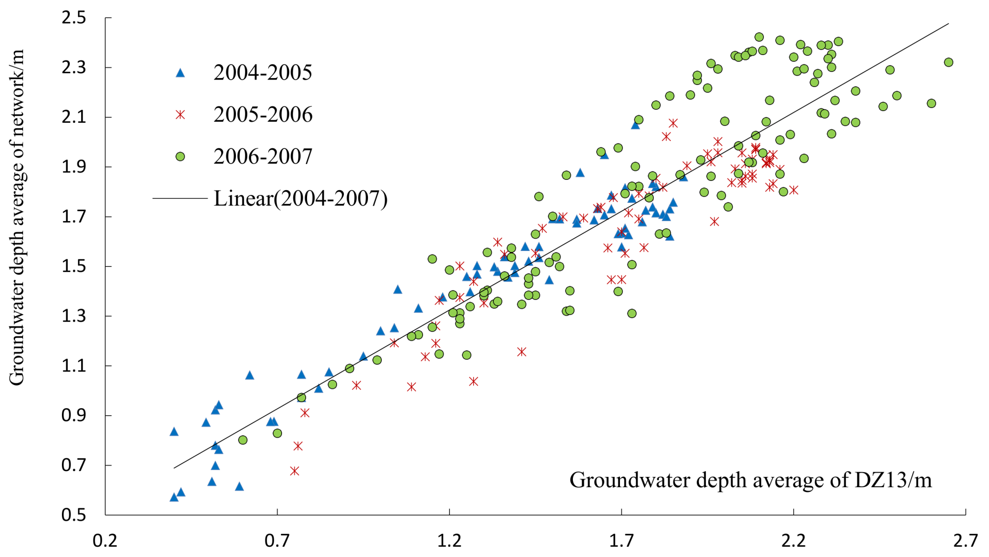
To determine if the representative locations accurately estimates the GD average, groundwater depth of the representative well measured every 5 days were compared to the GD average of all observation wells in the area at the corresponding date. Shown as in Figure 10.
Figure 10 and Table 4 contain the plots and statistics of the representative location in each period versus the whole observation network average for the entire data series. The GD of the representative station is slightly floating around the network average (Figure 10). There is a negligible difference (RMSE is 0.053 m/m). When we compare the mean between the representative station average and the network average of each period, the difference between the two estimates is about 0.022 m/m. The locations were identified, based on the GD (x) of which, the region mean (y) could be estimated by y = 0.795x + 0.371, as shown in Figure 10, and a paired t-test indicates they are equal at a 99% confidence level. This indicates that the DZ13 is a good representation of the study region with respect to groundwater depth during the experiment.
3.4.4. Validate the Satellite-Based DGWS
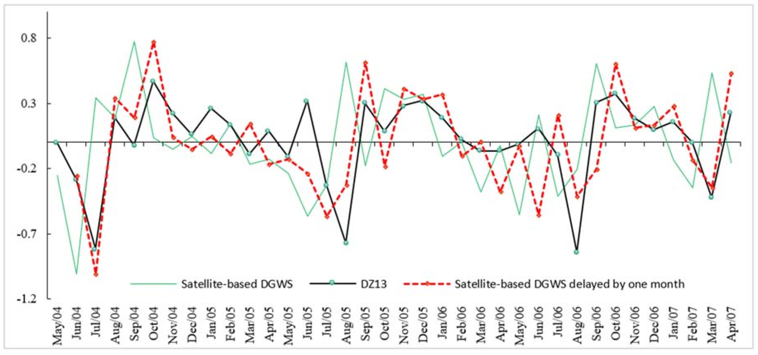
To test whether the representative point can adequately represent the entire area to validate the satellite-based DGWS, we compared three products of satellite-based DGWS (labeled Jpl, Gfz and Csr) with the DGWS of DZ13 and the average of all observation wells by the bivariate correlation analysis, respectively. The results are presented in Table 5. Frustratingly, their relevance is poor. However, when we delayed satellite-based DGWS by one month, their relevance was promoted to significant at the 0.01 level, and the results are shown in Table 5. The delayed products of satellite-based DGWS are labeled DJpl, DGfz and DCsr, respectively. The correlation between DZ13 and DGfz is the best, with a Pearson correlation value of 0.707. The time series of monthly GD change at representative point DZ13; Gfz and DGfz are presented as Figure 11.
Table 5 and Figure 11 shows that the correlation between DZ13 and satellite-based DGWS is similar to that of the average of all observation wells, indicating that DZ13 can replace the regional average to verify the satellite-based DGWS. There is no significant correlation between the observed data and the satellite-based data of DGWS in the current month, but significant correlation with the data delayed by one month. This phenomenon may be due to the hydrological characteristics of the study area. The study area is near the ocean and, due to the influence of the Yellow River and the sea, surface runoff is rich, and the soil moisture content is high. Therefore, the groundwater mainly comes from the recharge of the soil moisture and surface water, and the change of soil moisture and surface water strongly affects the change of GD. The more soil moisture and surface water, the smaller the groundwater depth. Generally, due to the recharge of the soil moisture to groundwater taking some time, and the satellite-based DGWS being derived from TWS change deducting soil moisture and surface water, there will be a time lag between the satellite-based DGWS and the measured GD. This also implies that the GRACE Level 3 products can be used to predict the GD in the area one month in advance.
4. Conclusions and Discussion
The following results can be summarized:
The groundwater depth in the Contemporary Yellow River Delta has obvious seasonal variation, and the GD is consistent with the change of surface water and precipitation in the area. The results of the spatial variability analysis found groundwater spatial depth variability in the study area was moderate. The monthly variation coefficient fluctuated from 24.96% to 73.04%. The variation coefficients of GD also have a seasonal aspect. In each year, the spatial coefficient of variation in the wet season was the largest while other months were relatively stable. The results of the correlation analysis showed that spatial variability of GD anomalies exhibits dependence on spatial mean of GD. The spatial variability of GD in wet season was generally stronger than in dry season. Research in other regions found similar results in soil moisture and water storage [20,29,30,31,32]. The results of this study are of great significance to the restoration of saline-alkali soil. In saline soil, the salt content of soil is not inseparable from the high mineral degree of groundwater, the smaller the spatial variability of groundwater depth, the more stable the salt content and the more favorable for plant growth. Therefore, the regulation of GD provides an important means to control the saline-alkali degree in the contemporary Yellow River Delta. A further possible implication is that the contribution of groundwater to local evapotranspiration and runoff is important under very wet and dry conditions. This may be a justification for incorporating groundwater into various type of water management systems.
The results of Spearman rank correlation analysis show that the GD demonstrates obvious temporal stability characteristics. The temporal stability of GD at different water levels will exhibit different temporal stability: more stable in time of normal water level than either in dry season or wet periods. Suggested reasons for differences in GD in dry and wet conditions include precipitation recharge, irrigation, vegetation root absorption, and strong surface evaporation. During the dry period, the evaporation of soil surface is strong, and the capillary movement of water in the soil cause groundwater level decline. At the same time, in areas where farms introduce the Yellow River water for irrigation, this artificially improves the groundwater level and thereby increases the temporal variability of GD. During wet and dry periods, precipitation and vegetation root uptake could differ. It is different with the soil moisture. For example, Martinez et al., using data from a network consisting of 23 soil moisture stations in 36 months (from June 1999 to May 2002) to study the soil moisture temporal stability in 1285 km2 located at the central part of the Douro Basin in Spain, found that soil moisture temporal stability during dry periods was always stronger than in wet ones. These authors also observed that the period with the lowest temporal stability coincided with the transition from dry to wet [33]. Williams et al., who sampled continuously throughout the year, found that soil moisture temporal stability was lower during the relatively dry period [34]. The divergence of the conclusions between the two fields shows that groundwater depth variations did not strictly followed soil moisture dynamics, leading to a certain decoupling between soil moisture and groundwater patterns in temporal stability.
The correlation analysis between Spearman rank correlation coefficient and time lags shows that the spatial pattern of GD is similar in a certain period, which is about 1.5–3 years in the study area, and the similarity will be weakened beyond this period. Similar results have been found in soil moisture. For example, Schneider and Martinez-Fernandez et al. found that the spatial pattern of soil moisture content was similar across 2–3 years, and the similarity decreased with increasing time interval [30,33].
The results of the representative stations of GD indicate that all the selected representative stations belong to a moderate grade of groundwater depth, but low depth and high depth of the station tends to be more unstable, indicating that the stations with medium depth often have a stronger temporal stability. The representative location is DZ13, with highest prediction accuracy, which implied a single sampling location could be used to estimate, and thus represent, the region mean. However, the relatively small spatial domain of the study area could account for this single representative point. For larger study areas, one representative point may be insufficient to estimate the mean GD of the whole region. Notwithstanding, it is obvious that temporal stability analysis could benefit future groundwater satellite products because it can verify stable GD networks as well as identify representative and anomalous sites, thus improving any ground validation programs.
As the bulk of current temporal stability research concentrates on soil moisture, it is useful to compare our study results in this area. It found that, although the groundwater is an important source of soil moisture, its temporal stability differs, likely due to other soil moisture factors at play. Further research is needed to verify this. In addition, the current research results show that while spatial scale influences soil moisture temporal stability, the extent of the impact remains unclear. This finding contrasts with Coppola et al., who found surface soil moisture temporal stability around 225–8800 m2 with low mean relative deviations (MRD), typically 20–60% [35]. On the coastal plain of the United States, Bosch et al. reported that MRD of the soil moisture in the scope of 3750 km2 is more than 200% [36], while Broccain, who investigated two larger area (178 and 242 km2), found that the range of MRD was only about 50% [11].
Finally, we compared the data serial of the GD from the representative location and the remote sensing data. The results indicated that the representative location can replace the regional average to verify the satellite-based DGWS. Satellites such as GRACE can forecast the groundwater depth at region scale, with the DGWS afforded by remote sensing providing valuable and convenient monitoring information. Nevertheless, the temporal stability of the GD at different spatial scale remains unresolved. Future studies are needed to answer this question.
Author Contributions
R.W., Y.L., H.M., Y.P. and L.D. conceived, designed and conducted the research but also collected and analyzed the data. S.H. reviewed and edited the paper. He also was the corresponding author.
Funding
National This research received no external funding from “Thirteen Five” Program (2017YFD0200702), Shandong “Double Tops” Program (SYL2017XTTD02), Shandong Key R & D Program (2017CXGC0306) and the Cultivate Plan Funds for Young Teacher and the Science and Technology Innovation Foundation for Youth of Shandong Agricultural University (No. 23694).
Acknowledgments
The data used in this study were acquired as part of the mission of NASA’s Earth Science Division and archived and distributed by the Goddard Earth Sciences (GES) Data and Information Services Center (DISC). Sincere thanks are also extended to China’s national science and technology infrastructure platform construction project: Earth system science data sharing platform to provide information support.
Conflicts of Interest
The authors declare no conflicts of interest.
References
- Kuang, W.; Liu, J.; Dong, J.; Chi, W.; Zhang, C. The rapid and massive urban and industrial land expansions in China between 1990 and 2010: A CLUD-based analysis of their trajectories, patterns, and drivers. Landsc. Urban Plan. 2016, 15, 21–22. [Google Scholar] [CrossRef]
- Liu, Y.; Fang, F.; Li, Y. Key issues of land use in china and implications for policy making. Land Use Policy 2014, 40, 6–12. [Google Scholar] [CrossRef]
- International Research and Training Center on Erosion and Sedimentation (IRTCES). Case Study on Utilization of Sediment Resource in the Lower Yellow River; International Research and Training Center on Erosion and Sedimentation: Beijing, China, 2010. [Google Scholar]
- Zhang, T.T.; Zeng, S.L.; Gao, Y.; Ouyang, Z.T.; Li, B.; Fang, C.M.; Zhao, B. Assessing impact of land uses on land salinization in the Yellow River Delta, China using an integrated and spatial statistical model. Land Use Policy 2011, 28, 857–866. [Google Scholar] [CrossRef]
- Fang, H.; Liu, G.; Kearney, M. Georelational analysis of soil type, soil salt content, landform, and land use in the Yellow River Delta, China. Environ. Manag. 2005, 35, 72–83. [Google Scholar] [CrossRef]
- Qinghua, Y.E.; Liu, G.; Tian, G.; Chen, S.; Huang, C.; Chen, S.; Liu, Q.; Chang, J.; Shi, Y. Geospatial-temporal analysis of land-use changes in the Yellow River Delta during the last 40 years. Sci. China Ser. D Earth Sci. 2004, 47, 1008–1024. [Google Scholar]
- Fan, X.M.; Liu, G.H.; Tang, Z.P. Analysis on main contributors influencing soil salinization of Yellow River Delta. J. Soil Water Conserv. 2010, 24, 139–144. [Google Scholar]
- Yao, R.; Yang, J. Quantitative analysis of spatial distribution pattern of soil salt accumulation in plough layer and shallow groundwater in the Yellow River Delta. Trans. Chin. Soc. Agric. Eng. 2007. [Google Scholar] [CrossRef]
- Eltahir, E.A.B.; Yeh, P.J.F. On the asymmetric response of aquifer water level to floods and droughts in Illinois. Water Resour. Res. 1999, 35, 1199–1217. [Google Scholar] [CrossRef] [Green Version]
- Famiglietti, J.S.; Ryu, D.; Berg, A.A.; Rodell, M.; Jackson, T.J. Field observations of soil moisture variability across scales. Water Resour. Res. 2008, 44. [Google Scholar] [CrossRef]
- Brocca, L.; Tullo, T.; Melone, F.; Moramarco, T.; Morbidelli, R. Catchment scale soil moisture spatial–temporal variability. J. Hydrol. 2012, 422–423, 63–75. [Google Scholar]
- Li, B.; Rodell, M. Spatial variability and its scale dependency of observed and modeled soil moisture under different climate conditions. Hydrol. Earth Syst. Sci. 2013, 17, 1177–1188. [Google Scholar] [CrossRef]
- Western, A.W.; Blöschl, G. On the spatial scaling of soil moisture. J. Hydrol. 1999, 217, 203–224. [Google Scholar] [CrossRef]
- Rodell, M.; Chen, J.; Kato, H.; Famiglietti, J.S.; Nigro, J.; Wilson, C.R. Estimating groundwater storage changes in the Mississippi River basin (USA) using GRACE. Hydrogeol. J. 2007, 15, 159–166. [Google Scholar] [CrossRef]
- Voss, K.A.; Famiglietti, J.S.; Lo, M.H.; Linage, C.D.; Rodell, M.; Swenson, S.C. Groundwater depletion in the middle east from GRACE with implications for transboundary water management in the Tigris-Euphrates-Western Iran region. Water Resour. Res. 2013, 49, 904–914. [Google Scholar] [CrossRef] [PubMed]
- Rowlands, D.D.; Luthcke, S.B.; Klosko, S.M.; Lemoine, F.G.R.; Chinn, D.S.; Mccarthy, J.J.; Cox, C.M.; Anderson, O.B. Resolving mass flux at high spatial and temporal resolution using GRACE intersatellite measurements. Geophys. Res. Lett. 2005, 32, 319–325. [Google Scholar] [CrossRef]
- Swenson, S.; Wahr, J. Post-processing removal of correlated errors in grace data. Geophys. Res. Lett. 2006, 33. [Google Scholar] [CrossRef]
- Vachaud, G.; Silans, A.P.D.; Balabanis, P.; Vauclin, M. Temporal stability of spatially measured soil water probability density function. Soil Sci. Soc. Am. J. 1985, 49, 822–828. [Google Scholar] [CrossRef]
- Kachanoski, R.G.; Jong, E.D. Scale dependence and the temporal persistence of spatial patterns of soil water storage. Water Resour. Res. 1988, 24, 85–91. [Google Scholar] [CrossRef]
- Penna, D.; Brocca, L.; Borga, M.; Fontana, G.D. Soil moisture temporal stability at different depths on two alpine hillslopes during wet and dry periods. J. Hydrol. 2013, 477, 55–71. [Google Scholar] [CrossRef]
- Blöschl, G.; Wagner, W. Remote Sensing in Hydrology and Water Management; Springer: Berlin, Germany, 2009. [Google Scholar]
- Grayson, R.B.; Western, A.W. Towards areal estimation of soil water content from point measurements: Time and space stability of mean response. J. Hydrol. 1998, 207, 68–82. [Google Scholar] [CrossRef]
- Dumedah, G.; Coulibaly, P. Evaluation of statistical methods for infilling missing values in high-resolution soil moisture data. J. Hydrol. 2011, 400, 95–102. [Google Scholar] [CrossRef]
- Zhao, Y.M.; Song, C.S. Scientific Survey of the Yellow River Delta National Nature Reserve; China Forestry Publishing House: Beijing, China, 1995. [Google Scholar]
- Nielsen, D.R.; Bouma, J. Soil Spatial Variability; Pudoc: Wageningen, The Netherlands, 1985. [Google Scholar]
- Brocca, L.; Melone, F.; Moramarco, T.; Morbidelli, R. Soil moisture temporal stability over experimental areas in central Italy. Geoderma 2009, 148, 364–374. [Google Scholar] [CrossRef]
- Heathman, G.C.; Larose, M.; Cosh, M.H.; Bindlish, R. Surface and profile soil moisture spatio-temporal analysis during an excessive rainfall period in the Southern Great Plains, USA. Catena 2009, 78, 159–169. [Google Scholar] [CrossRef]
- Gao, L.; Shao, M. Temporal stability of shallow soil water content for three adjacent transects on a hillslope. Agric. Water Manag. 2012, 110, 41–54. [Google Scholar] [CrossRef]
- Gao, L.; Shao, M. Temporal stability of soil water storage in diverse soil layers. Catena 2012, 95, 24–32. [Google Scholar] [CrossRef]
- Schneider, K.; Huisman, J.A.; Breuer, L.; Zhao, Y.; Frede, H.G. Temporal stability of soil moisture in various semi-arid steppe ecosystems and its application in remote sensing. J. Hydrol. 2008, 359, 16–29. [Google Scholar] [CrossRef]
- Biswas, A.; Si, B.C. Identifying scale specific controls of soil water storage in a hummocky landscape using wavelet coherency. Geoderma 2011, 165, 50–59. [Google Scholar] [CrossRef]
- Jia, Y.H.; Shao, M.A. Temporal stability of soil water storage under four types of revegetation on the northern Loess Plateau of China. Agric. Water Manag. 2013, 117, 33–42. [Google Scholar] [CrossRef]
- Martínezfernández, J.; Ceballos, A. Temporal stability of soil moisture in a large-field experiment in Spain. Soil Sci. Soc. Am. J. 2003, 67, 1647–1656. [Google Scholar] [CrossRef]
- Williams, C.J.; Mcnamara, J.P.; Chandler, D.G. Controls on the temporal and spatial variability of soil moisture in a mountainous landscape: The signature of snow and complex terrain. Hydrol. Earth Syst. Sci. 2009, 13, 1325–1336. [Google Scholar] [CrossRef]
- Coppola, A.; Comegna, A.; Dragonetti, G.; Lamaddalena, N.; Kader, A.M.; Comegna, V. Average moisture saturation effects on temporal stability of soil water spatial distribution at field scale. Soil Tillage Res. 2011, 114, 155–164. [Google Scholar] [CrossRef]
- Bosch, D.D.; Lakshmi, V.; Jackson, T.J.; Choi, M.; Jacobs, J.M. Large scale measurements of soil moisture for validation of remotely sensed data: Georgia soil moisture experiment of 2003. J. Hydrol. 2006, 323, 120–137. [Google Scholar] [CrossRef]
Figure 1.
Spatial distribution of the observation wells in the study area. (A) The wells listed on the landsat8 color image composited by Bands 543; (B) The wells listed on the elevation map.
Figure 1.
Spatial distribution of the observation wells in the study area. (A) The wells listed on the landsat8 color image composited by Bands 543; (B) The wells listed on the elevation map.

Figure 2.
Sequence diagram of groundwater depth survey from 2004–2007.

Figure 3.
Seasonal distribution of groundwater depth.

Figure 4.
Spatial variation coefficient of groundwater depth of each month in 2004–2007.
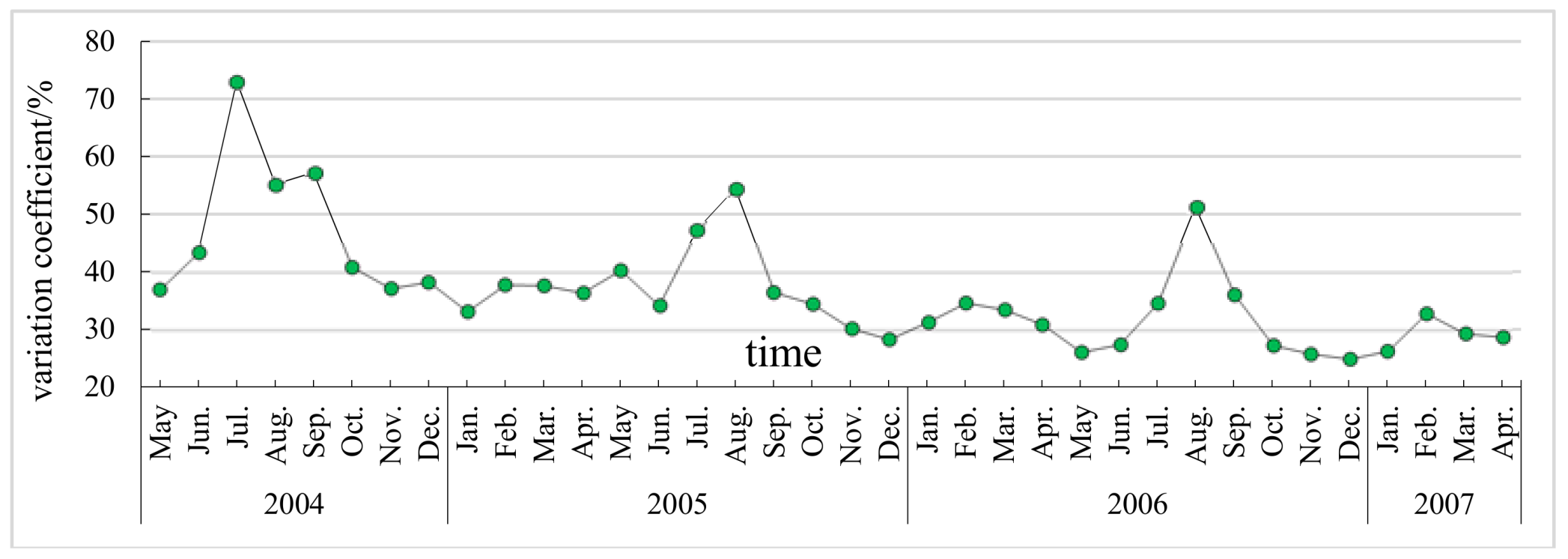
Figure 5.
Interpolated map (IDW) of mean groundwater depth in January and August 2005. (a) Groundwater depth in January; (b) Groundwater depth in August.
Figure 5.
Interpolated map (IDW) of mean groundwater depth in January and August 2005. (a) Groundwater depth in January; (b) Groundwater depth in August.

Figure 6.
Relationship between groundwater depth and variation coefficient.

Figure 7.
Scatter plot of Spearman rank correlation coefficient and groundwater depth.

Figure 8.
Mean relative difference and standard deviation of groundwater depth for different time part of each survey well. Note: Vertical bars represent standard deviation. Representative locations are marked in black. Vertical bars correspond to ±one standard deviation of the relative difference (%) over time.
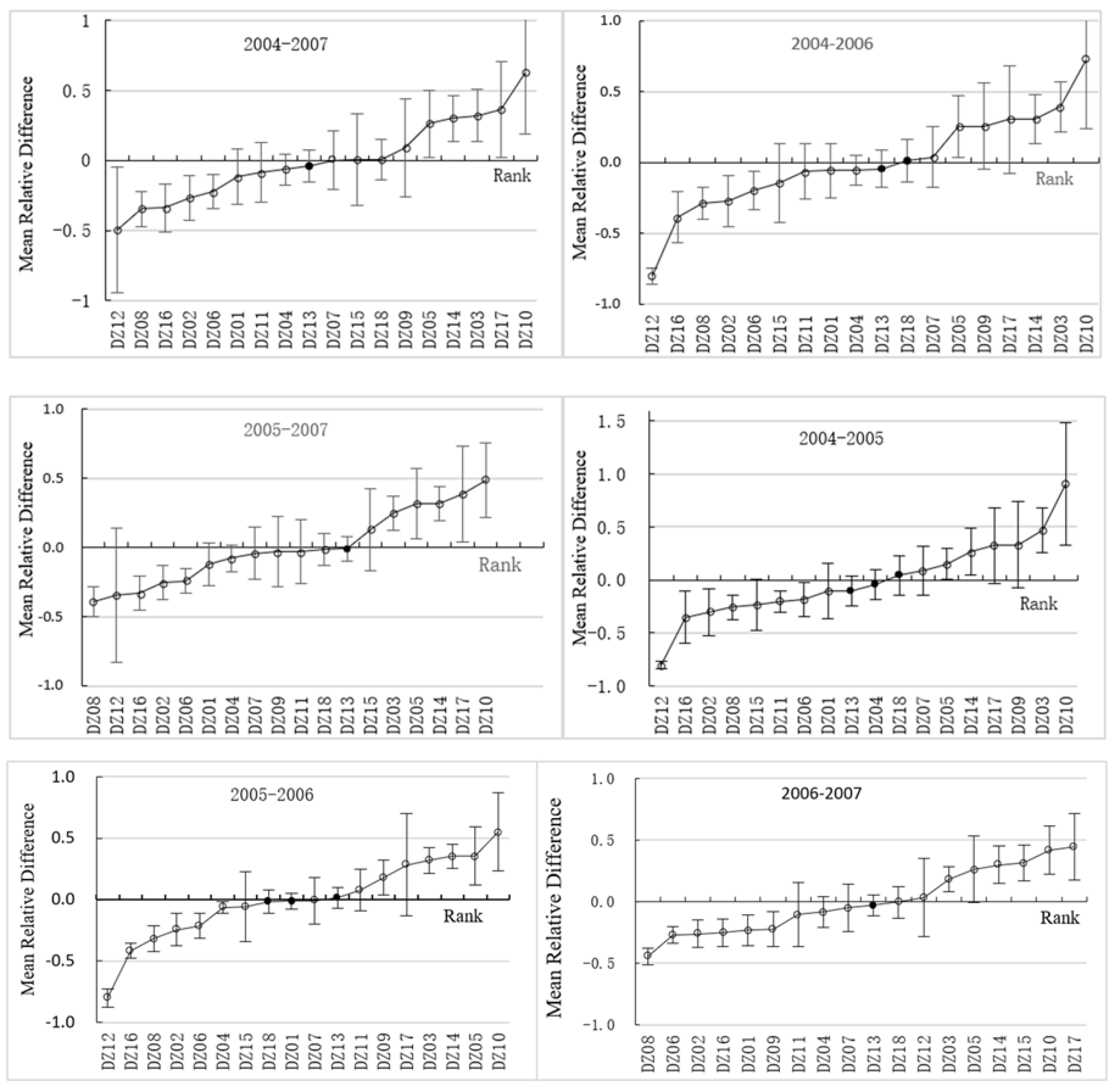
Figure 9.
The locations of DZ01/DZ04/DZ13/DZ18.

Figure 10.
Correlation between the representative location and mean of the whole region for groundwater depth in 2004–2007 (259 samples).
Figure 10.
Correlation between the representative location and mean of the whole region for groundwater depth in 2004–2007 (259 samples).

Figure 11.
Time series of DZ13and the satellite-based DGWS for monthly groundwater depth change in 2004–2007 (Note: The present values of the satellite-based DGWS and the satellite-based DGWS delayed by one month are 0.1 times the original value).
Figure 11.
Time series of DZ13and the satellite-based DGWS for monthly groundwater depth change in 2004–2007 (Note: The present values of the satellite-based DGWS and the satellite-based DGWS delayed by one month are 0.1 times the original value).


Table 1.
Spearman rank correlation coefficient of past months.
| Month | 2004–2005 | 2005–2006 | 2006–2007 | |||||||||
|---|---|---|---|---|---|---|---|---|---|---|---|---|
| May | August | December | February | April | August | December | February | April | August | December | February | |
| May | 1.000 | 0.521 * | 0.676 ** | 0.616 ** | 0.732 ** | 0.470 * | 0.299 | 0.443 * | 0.389 | 0.378 | 0.294 | 0.298 |
| August | 1.000 | 0.620 ** | 0.550 ** | 0.556 ** | 0.613 ** | 0.464 * | 0.342 | 0.461 * | 0.087 | −0.121 | 0.096 | |
| December | 1.000 | 0.953 ** | 0.876 ** | 0.753 ** | 0.673 ** | 0.732 ** | 0.645 ** | 0.518 * | 0.428 * | 0.531 * | ||
| February | 1.000 | 0.851 ** | 0.623 ** | 0.781 ** | 0.783 ** | 0.738 ** | 0.488 * | 0.455 * | 0.577 ** | |||
| April | 1.000 | 0.609 ** | 0.602 ** | 0.680 ** | 0.740 ** | 0.488 * | 0.329 | 0.476 * | ||||
| August | 1.000 | 0.549 ** | 0.644 ** | 0.449 * | 0.563 ** | 0.190 | 0.250 | |||||
| December | 1.000 | 0.874 ** | 0.874 ** | 0.488 * | 0.320 | 0.461 * | ||||||
| February | 1.000 | 0.866 ** | 0.775 ** | 0.579 ** | 0.635 ** | |||||||
| April | 1.000 | 0.539 * | 0.366 | 0.513 * | ||||||||
| August | 1.000 | 0.804 ** | 0.808 ** | |||||||||
| December | 1.000 | 0.833 ** | ||||||||||
| February | 1.000 | |||||||||||
| Sum/month | 17 | 16 | 24 | 24 | 25 | 20 | 24 | 30 | 20 | 16 | 12 | 12 |
Note: Due to the table is too large, only a few months in the table; Sum: the time interval reached the significant level; ** Statistical significance at p < 0.01, * Statistical significance at p < 0.05.
Table 2.
The determination coefficient of Spearman rank correlation coefficient and the time lags.
| 2004-2005 | May | June | July | August | September | October | November | December | January | February | March | April |
|---|---|---|---|---|---|---|---|---|---|---|---|---|
| Pearson coefficient | −0.799 ** | −0.610 ** | −0.815 ** | −0.856 ** | −0.865 ** | −0.855 ** | −0.789 ** | −0.789 ** | −0.676 ** | −0.716 ** | −0.757 ** | −0.749 ** |
| 2005–2006 | May | June | July | August | September | October | November | December | January | February | March | April |
| Pearson coefficient | −0.781 ** | −0.691 ** | −0.778 ** | −0.754 ** | −0.722 ** | −0.745 ** | −0.676 ** | −0.712 ** | −0.740 ** | −0.758 ** | −0.540 ** | −0.438 ** |
| 2006–2007 | May | June | July | August | September | October | November | December | January | February | March | April |
| Pearson coefficient | −0.707 ** | −0.735 ** | −0.771 ** | −0.816 ** | −0.776 ** | −0.801 ** | −0.820 ** | −0.816 ** | −0.851 ** | −0.839 ** | −0.634 ** | −0.574 ** |
** Statistical significance at p < 0.01.
Table 3.
Representative locations in different time scales.
| Time Scale | Representative Locations | Unstable Locations | ||
|---|---|---|---|---|
| Well Code | Groundwater Depth Grade | Well Code | Groundwater Depthm and Grade | |
| 2004–2007 | DZ13 | medium | DZ12 and DZ10 | 0.95 higher and 2.60 lower |
| 2004–2006 | DZ13, DZ18 | medium | DZ12 and DZ10 | 0.95 higher and 2.60 lower |
| 2005–2007 | DZ13 | medium | DZ12 and DZ10 | 0.95 higher and 2.60 lower |
| 2004–2005 | DZ04, DZ13 and DZ18 | medium | DZ12 and DZ10 | 0.95 higher and 2.60 lower |
| 2005–2006 | DZ13, DZ01 and DZ18 | medium | DZ12 and DZ10 | 0.95 higher and 2.60 lower |
| May 2006–24 December 2007 | DZ13 | medium | DZ08 and DZ10 | 1.08 higher and 2.60 lower |
Table 4.
Comparison between the representative location and mean of the whole region for groundwater depth in different period.
Table 4.
Comparison between the representative location and mean of the whole region for groundwater depth in different period.
| Period | Pearson Correlation | Mean of the DZ13/m | Mean of the Region/m | Difference/m/m |
|---|---|---|---|---|
| 5 May 2004–28 April 2005 | 0.961 ** | 1.294 | 1.419 | 0.088 |
| 2 May 2005–27 April 2006 | 0.910 ** | 1.707 | 1.670 | −0.022 |
| 2 May 2006–2 December 2007 | 0.898 ** | 1.782 | 1.812 | 0.017 |
| 5 May 2004–27 April 2006 | 0.943 ** | 1.501 | 1.544 | 0.028 |
| 2 May 2005–2 December 2007 | 0 | 1.754 | 1.759 | 0.003 |
| 5 May 2004–2 December 2007 | 0.924 ** | 1.629 | 1.665 | 0.022 |
** Significant at 0.01 level (two tails).
Table 5.
The Pearson Correlation of DGWS from satellite-based data, DZ13 and the average of all wells.
Table 5.
The Pearson Correlation of DGWS from satellite-based data, DZ13 and the average of all wells.
| Jpl | Gfz | Csr | DJpl | DGfz | DCsr | |
|---|---|---|---|---|---|---|
| DZ13 | 0.081 | −0.049 | 0.031 | 0.673 ** | 0.707 ** | 0.635 ** |
| All wells | 0.089 | −0.033 | 0.044 | 0.634 ** | 0.644 ** | 0.566 ** |
** Significant at 0.01 level (two tails).
© 2018 by the authors. Licensee MDPI, Basel, Switzerland. This article is an open access article distributed under the terms and conditions of the Creative Commons Attribution (CC BY) license (http://creativecommons.org/licenses/by/4.0/).
Share and Cite
MDPI and ACS Style
Wang, R.; Huston, S.; Li, Y.; Ma, H.; Peng, Y.; Ding, L. Temporal Stability of Groundwater Depth in the Contemporary Yellow River Delta, Eastern China. Sustainability 2018, 10, 2224. https://doi.org/10.3390/su10072224
AMA Style
Wang R, Huston S, Li Y, Ma H, Peng Y, Ding L. Temporal Stability of Groundwater Depth in the Contemporary Yellow River Delta, Eastern China. Sustainability. 2018; 10(7):2224. https://doi.org/10.3390/su10072224
Chicago/Turabian StyleWang, Ruiyan, Simon Huston, Yuhuan Li, Huiping Ma, Yang Peng, and Lihua Ding. 2018. "Temporal Stability of Groundwater Depth in the Contemporary Yellow River Delta, Eastern China" Sustainability 10, no. 7: 2224. https://doi.org/10.3390/su10072224
Note that from the first issue of 2016, this journal uses article numbers instead of page numbers. See further details here.