How Foreign Direct Investment Influences Carbon Emissions, Based on the Empirical Analysis of Chinese Urban Data

Abstract

The overabundance of carbon emissions is widely considered as a serious world problem. This paper focuses on analyzing the influence of economic factors on carbon emissions. Based on the traditional STIRPAT model, in terms of the “pollution haven hypothesis” and “pollution halo hypothesis”, this paper employs the dynamic panel data model to explore the impact of economic elements such as economic growth, population, foreign direct investment and others on carbon emissions. Based on our research, China’s urban carbon emissions do not follow the inverted U-shaped hypothesis of the traditional EKC curve theory and presents an inverted N-type. Moreover, current foreign direct investment increases the carbon emissions of Chinese cities due to the “implicit trade carbon”. However, during the lagging period of one phase, it significantly reduced urban carbon emissions. In addition, the lag of one period of carbon emissions statistically led to carbon emissions at the current stage. According to the empirical analysis results, this paper proposes some reasonable improvements for carbon dioxide emission reduction, which have certain reference values for other developing countries facing similar carbon emission reduction challenges.

1. Introduction

How the economy sustains development under the dual effects of limited energy resources and environmental pollution is one of the most interesting research areas in macroeconomics and resource energy economics. As the most basic foundation for economic growth and social development, energy plays an irreplaceable role in modern economic systems. The role of renewable sources continues to be the fastest growing power source in the global power mix. Bioenergy may provide roughly 10% of global supplies and accounts for roughly 80% of the energy derived from renewable sources [1]. Renewable energy is considered to be an important factor input in future sustainable development. Countries have gradually realized the importance of this energy technology. The European Union has set itself the ambitious target of increasing the share of renewable sources in final energy consumption to 20% by 2020 (Data Resources: https://ec.europa.eu/clima/policies/strategies/2020_en). In the largest energy-consuming countries, China has also increasingly paid attention to sustainable development and increased the development and utilization of renewable energy. China’s clean energy data show that the proportion of clean energy and renewable energy production such as hydropower, nuclear power and wind power in total energy production increased from 3.1% in 1978 to 10.3% in 2012 (Data Resources: National Bureau of Statistics of People’s Republic of China). In addition, clean energy power generation such as hydropower, nuclear power, wind power, and solar power generated a growth of 11.8% in the first three quarters of 2018, which was 3.8 percentage points higher than the growth rate of all power generation, accounting for 22.9% of all power generation, and a 0.8% increase over the same period of last year. Its power generation energy structure continues to be optimized (Data Resources: National Bureau of Statistics of People’s Republic of China).

However, in the near future, there is no doubt that global renewable electricity generation is expected to surpass natural gas. Popp et al. [2] pointed out that energy consumption is still increasing rapidly, with an approximate 570 EJ consumed at the primary energy level in 2014. The world gets about 19.2% of its energy from renewables, including about 8.9% from traditional biomass and about 10.3% from modern renewables. However, the current situation is still that most heat and power used today mainly comes from biomass, especially fossil fuel [1]. Continuous reliance on fossil fuels makes it very difficult to reduce emissions of greenhouse gases. Global energy demand has increased by 2.1% in 2017, compared to 0.9% in 2016. Moreover, global carbon emissions increased by net 460 more million tons of carbon dioxide and reached 32.5 billion tons in 2017 (Data Resources: International Energy Agency).

Since the reform and opening up, while maintaining a high-speed economic growth, China is also facing an increasingly serious environmental climate challenge. At present, excessive carbon dioxide emissions have become a major constraint on economic growth and the overall welfare of the community. According to the “National Environmental Analysis of the People’s Republic of China” published jointly by the Asian Development Bank and Tsinghua University, in the 500 largest cities in China, less than 1% of the air quality standards recommended by the World Health Organization (WHO, Geneva, Switzerland) have been achieved. Among the 10 cities with the most serious environmental pollution in the world, 7 are in China. China has become one of the countries with the most serious environmental pollution in the world.

In recent years, China has been vigorously advancing carbon emission reduction policies and measures, including the macroeconomic modernization system, supply-side structural reforms, seeking green development, building green GDP, and improving economic quality. The Chinese government has also gradually increased its environmental protection and environmental law enforcement. The Party’s 18th National Congress also put its ecological civilization construction on a strategic position with the overall layout of the “five in one” socialism with Chinese characteristics. According to incomplete statistics, in 2014, there were 897 written instructions from the central leaders on environmental protection work and 557 instructions are directly related to the key work of the Ministry of Environmental Protection. The Politburo Standing Committee of the Politburo had made relevant instructions [3]. The overall goal of the “13th Five-Year Plan for Controlling Greenhouse Gas Emissions” states that by 2020, per unit GDP of CO₂ emissions will fall by 18% compared to 2015, and the total amount of carbon emissions will be effectively controlled. The Chinese government sets a binding target to propose a reduction in carbon emissions per unit of GDP from 40–45% in 2020 compared with 2005 (Data Resources: The United Nations Climate Change conference, 2009).

As the country with the largest carbon emission and the country that is facing the greatest constraint on carbon emission reduction, China has an arduous task in dealing with global climate change. The in-depth exploration of the potential drivers of CO₂ emission growth in the context of Chinese economic development has important theoretical and practical significance for climate change, the development of a low-carbon economy, and the construction of ecological civilization.

In terms of the statistics of the Ministry of Commerce of China, there were 35,652 foreign-invested enterprises newly established in China in 2017. The actual use of foreign capital was 877.6 billion yuan (USD 131 billion), representing an increase of 7.9% (Data Resources: Ministry of Commerce of the People’s Republic of China). At the same time, the use of foreign capital is also diversifying. The relevant empirical data shows that Chinese attraction of foreign direct investment (FDI) and domestic enterprises’ outward direct investment (OFDI) shows a parallel growth trend. In 2014, China OFDI amounted to USD 123.1 billion. The amount of actual utilization of FDI was USD 115.56 billion, both hitting a record high. At the same time, the scale of OFDI by Chinese companies exceeded the scale of FDI attracted by China for the first time, which made the two-way investment approach balance for the first time (Data Resources: Ministry of Commerce of the People’s Republic of China, <2014 Statistical Bulletin on China’s Outward Foreign Direct Investment>). Since then, the scale of Chinese OFDI has accelerated at a high speed and reached UDS 196.15 billion, with a 34.7% increase and 13.5% share of global, compared with the amount of FDI of USD 126 billion. In addition, the amount of OFDI exceeded FDI by USD 70.15 billion (Data Resources: Ministry of Commerce of the People’s Republic of China).

The classical theory of development economics holds that the main role of FDI in developing countries is to make up for capital gaps and promote technological progress. FDI is a “complex” of capital, technology, organization, and marketing networks. According to the theory of heterogeneous corporate trade, enterprises with direct foreign investment have higher fixed costs. Enterprises with the lowest productivity choose to produce and sell products in the country. Those with medium productivity will choose to export services to the international market. Only the highest productivity in the industry is possible for companies to invest in FDI [4,5]. Therefore, foreign-invested companies usually have higher levels of production technology and invest more R&D expenditures, which will result in horizontal spillovers within the industry and vertical spillovers between industries in local host countries, which in turn will increase the productivity of companies [6,7].

The Chinese economy has rapidly grown and companies have also shortened the gap with international advanced production technologies, among which FDI has played an irreplaceable role in export trade development [8,9], and in technological progress and productivity improvement [6]. Based on the data from 1995 to 2013, foreign-funded enterprises contributed around 16% to 34% of Chinese GDP, and contributed around 11% to 29% of Chinese employment, of which the 2013 figures were 33% and 27% respectively [10].

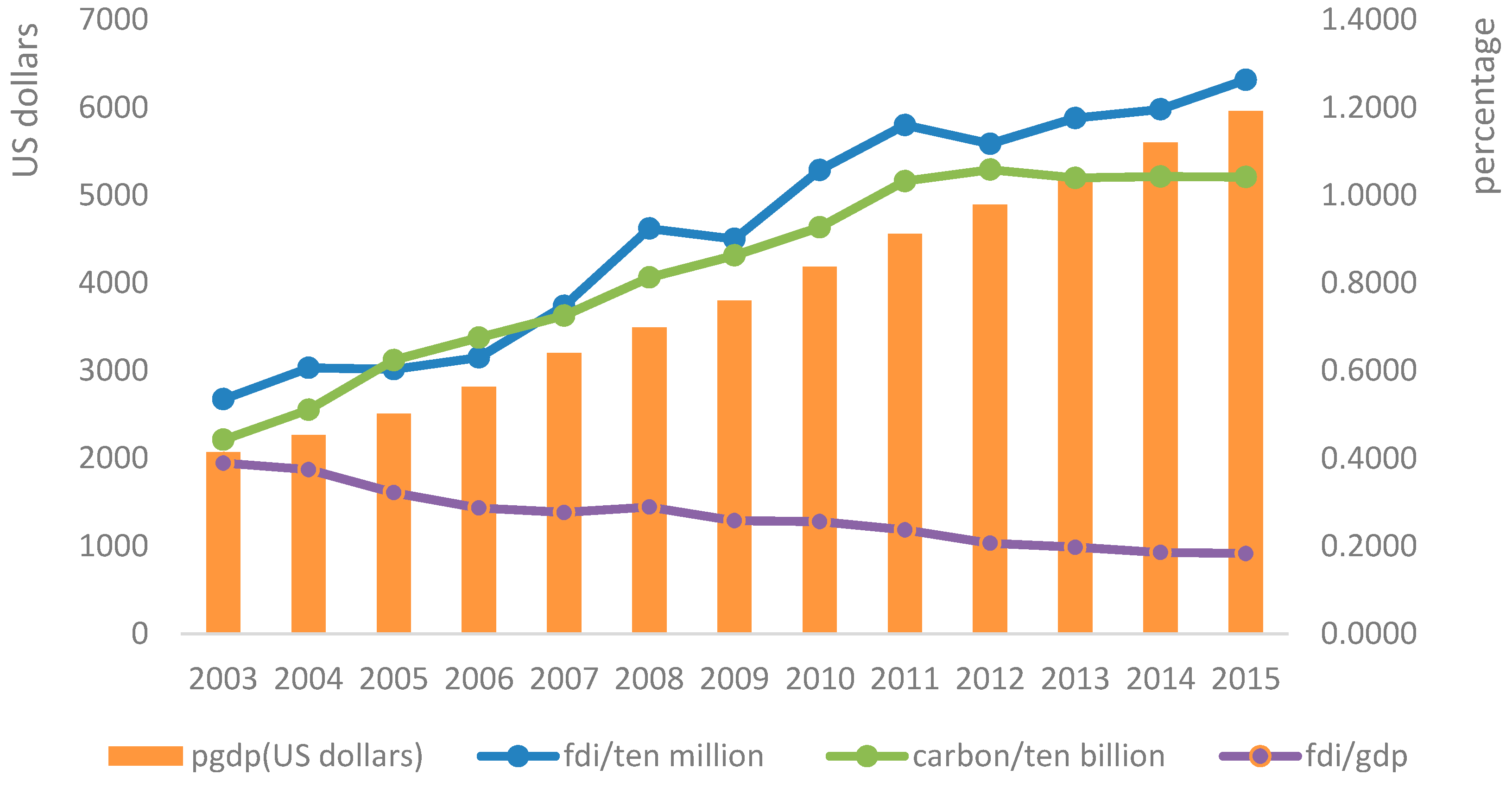
However, with the rapid increase in the scale of foreign investment in China, the contradiction between Chinese economic growth and the deterioration of the ecological environment is increasing. According to the Pollution Haven Hypothesis (PHH), FDI helps China introduce capital to promote industrial upgrading, and it may also be intensifying local environmental pollution to generate a “pollution paradise”. Figure 1 shows the main data and we can see that the country’s CO₂ emissions and FDI share have maintained a trend of sustained growth. The average growth rate reached 8.19% and 6.51% respectively. Under this background, the in-depth study of the “Pollution Paradise Hypothesis” and the influencing factors behind it, combined with Chinese current economic conditions, clearly has important academic and practical significance. It helps us further improve Chinese opening up and environmental supervision mechanism for investment promotion and will also provide reference for policy authorities on future energy and environmental economic policy choices and arrangements.

This paper is organized as follows: the second part discusses the current review of potential influencing factors and measurements for carbon emissions; the third part is in the light of EKC theory and STIRPAT model and establishes a delayed first-order differential Generalized Method of Moments (GMM) and Sys GMM model using panel data; the fourth part is for empirical analysis; and the fifth part is conclusions and policy recommendations.

2. Literature Review

2.1. EKC Literature Review

With the increasingly significant impact of environmental issues on people’s production and life, the stable growth of social economy is facing great challenges. The 2010 Cancun Climate Conference agreed to limit global warming to 2 °C in this century (The 16th Conference of Parties of the United Nations Framework Convention on Climate Change), which encourages more analysis of economic influencing factors for carbon emission reduction. The United Nations Environment Programme (UNEP) published “The Emissions Gap Report 2014” and pointed out some important factors, for example, subsidies that encourage the use of fossil fuel, water, and other scarce resources; investments that are driven by short-term returns in traditional high-carbon sectors and practices; and lack of investment in low-carbon, resource-efficient solutions. It also mentions that imperfect information, split incentives, and externalities are important market barriers to energy efficiency. However, not all empirical analysis supports the positive relationship between temperature difference and CO₂ concentration [11].

Traditional economic research directions include economic growth, industrial structure, technological progress, foreign trade, regional trade, and population migration etc. In addition, current research investigates more potential factors such as the transition of input factors. Chen et al. [12] substituted renewable energy production for fossil fuels and built an energy environment and non-radial Malmquist index to measure carbon emissions. One of these significant topics is research on the relationship between economic growth and environment, which is called the environmental Kuznets curve. EKC theory was first proposed and expanded by Grossman and Krueger [13,14]. The World Development Report 1992 adopted empirical research to demonstrate its existence. EKC theory says an increase in economic growth will engender environmental pressure at first, but after a turning point, rising in economic growth will decrease environmental pressure. Although scholars have recently performed many empirical analyses on EKC shapes, they are still widely used to test environmental quality and economic growth. Apergis and Ozturk [15] employed GMM methodology to EKC hypothesis on 14 Asian countries from 1990 to 2011 and found the turning points of the U-shaped EKC. Najid Ahmad et al. [16] applied autoregressive distributed Lag (ARDL) and VECM methodology to display an inverted U-shaped relationship between CO₂ emissions and economic growth in Croatia from 1992 to 2011. China is a fast-developing country with high speed of economic growth and many scholars are curious about the relationship between its economic growth and its environment pollutants such as SO₂ and CO₂. Diao et al. [17], Wang et al. [18], Yin et al. [19], Li et al. [20] adopted static or dynamic panel data analytic methods to study the existence of KEC hypothesis based on China provencial data.

2.2. FDI Literature

The influence of FDI and foreign trade on carbon emissions has been increasingly valued by academic research institutes. Traditional scholars hold the idea that FDI will further deepen the deterioration of the environment. Taylor and Copeland proposed the “Pollution Shelter Hypothesis”, which states that national environmental regulations have reduced the competitiveness of domestic polluting enterprises and led to the transfer of industries. Pollution-intensive companies will move from countries with high levels of internalization of environmental costs to low levels. The country’s migration has led to the implementation of lower environmental standards in countries that have become refuges for pollution-intensive industries [21]. Levinson and Taylor [22] used theory and empirics to examine the effect of environmental regulations on trade flows and they find industries whose abatement costs increased most experienced the largest increases in net imports. Guo Kesha et al.’s [23] study showed that large amounts of foreign capital provide necessary technical and financial support for industrial economic adjustment and changes in economic growth patterns; carbon leakage has weakened the effectiveness of emission reduction policies in developed countries and may even lead to an increase in global carbon emissions.

The effects brought by the hypothesis to the host country’s environment is called the “pollution halo hypothesis”. Based on this hypothesis, advanced clean technologies and environmental management systems used during foreign investment process will spread to the host country, which will have a favorable impact on the host country’s environment. The competition between domestic and foreign-funded enterprises will form a virtuous circle of “spiral ascent” and effectively promote the technology spillover and diffusion process of FDI enterprises. When transnational corporations invest in other countries, the environmental pollution problems faced by domestic companies in the host country are solved by increasing the efficiency of the use of resources. On the one hand, the development of environmental technologies in host countries is promoted through knowledge diffusion, technological spillovers and transfer, and capital investment. The investments of transnational corporations have promoted the economic development and technological progress of the host countries, brought a positive influence to the host country environment, and promoted the environmental cooperation between the countries in a deeper level. Zhu et al. [24] used panel data from five countries in Malaysia, India, the Philippines, Thailand, and Singapore in 1981–2011 to discover that the effect of FDI on carbon emissions is negative in countries with medium and high carbon emissions through panel quartile regression methods which supports the “halo effect hypothesis”. In addition, Atici [25] researched Asian countries also concluded that FDI is conducive to Asian countries reducing pollution. Jorgenson et al. [26] used panel data from 39 underdeveloped countries from 1975 to 2000 to examine the relationship between FDI and carbon emissions for host countries. The results confirmed that FDI has a significant negative effect on carbon emissions from underdeveloped countries.

Chinese scholars have used different measurement methods and research perspectives based on various sample data to test whether the FDI “contaminated shelter” hypothesis is established in China but have come to different conclusions. There are three main reasons for this. First, most of the existing literature uses provincial data. Research from the prefecture level is relatively rare, and prefectural-level city data have more research value than provincial-level data. This is because of the consolidation of provincial-level data. There are many regional differences in information, and prefecture-level cities can reflect the heterogeneity between regions on a smaller geographic scale. Second, most of the existing literature has selected one or more pollutant emissions, such as carbon dioxide, sulfur dioxide, and other gas emissions as a measure of environmental pollution. However, the selection of different pollutants will make the conclusions of the research contradictory. Although Xu et al. [27] constructed an environmental pollution comprehensive index through the entropy method and made up for the inadequacy of a single indicator, there are still some unconsidered issues for missing pollutants, such as PM_2.5. In addition, the main problem with adopting weighted composite indicators to measure environmental pollution is too difficult to find the weighted weights of objective authority. The unreasonable selection of environmental pollution indicators can weaken the explanatory power of the model. Finally, there are relatively few spatial measurement methods used in the existing research. Although some scholars use the spatial lag model, they ignore the huge differences in the regional space. The traditional measurement method assumes that the space is homogeneous and non-differentiated. Therefore, the estimated coefficient of the model is also fixed, which obviously violates the obvious fact of regional differences in China.

In this paper, the carbon impact factors are taken as the research object, and the generalized methods of moment estimation is used to systematically examine the key influencing factors of carbon emissions over 285 cities in China. The main contributions of this paper are as follows: First, this paper uses the characteristic data of Chinese cities as the research basis and discusses the factors affecting carbon emissions in more detail. Secondly, based on the STIRPART model and the EKC, this paper constructs a dynamic panel GMM model, which can effectively consider the time lag effect of each city in the process of social and economic development. Finally, according to the specificity of the industrialization process where Chinese economic development is located, this paper adds some factors to the economic growth factor, including FDI, labor output, secondary industry structure, and population. An inverted N-type KEC curve is discussed and FDI in the current period and the lagging period of one phase are also analyzed. The purpose of this paper is to sum up a series of exploratory research work, investigating the characteristics of carbon emissions based on urban aspects in China, exploring the specific relationship between carbon emissions and economic growth, and identifying the key factors of emissions to rationalize energy conservation and emission reduction policies for all cities in China and to effectively formulate and implement the necessary empirical support and decision-making basis.

3. Methodology Section

3.1. Data and Variables

China Business News divides China excluding Hong Kong, Macau, and Taiwan into 338 cities in five categories. Due to the availability and accessibility of the data set, this paper takes data of 285 cities from 2003 to 2015 into consideration. Data are derived from China Statistical Yearbook, China Urban Statistical Yearbook, EPS database and Wind database.

Table 1. Description of Variables.

Symbol	Variable	Definition	Unit
Carbon	City’s total CO2 emissions for each city annually	CO2 emissions from fossil fuels and the manufacture of cement	Ten Kiloton
P	Population for each city annually	Year-end population	Ten Thousand
IS	Industry structure for each city annually	percentage of the secondary industry GDP covering total GDP	%
PGDP	Gross domestic product for each city annually	Per Capita GDP	yuan per person
PGDP2	The square of GDP for each city annually	The square of Per Capita GDP	yuan per person
PGDP3	The cubic of GDP for each city annually	The cubic term of Per Capita GDP	yuan per person
FDI	Foreign direct investment for each city annually	The percentage of the FDI in the city’s GDP	%
T	Technical for each city annually	proportion of capital and labor	%

Notes: Data sources, the EPS database, China Statistical Yearbook, China Urban Statistical Yearbook.

provides a brief description of each variable used in this paper. Chinese statistical agencies did not publish CO₂ emissions data, according to the reference method provided by the Intergovernmental Panel on Climate Change (IPCC, Geneva, Switzerland) guidance catalogue and the Chinese CO₂ emissions estimated from data from the EPS database and Wind database.

Table 2. The Descriptive Statistics of Variables.

Variable	Obs.	Mean	Std. Dev.	Min	Max
Carbon	3705	5.748	1.323	−0.478	9.623
Capita PGDP	3694	10.017	0.820	4.560	13.056
(Capita PGDP)2	3694	101.023	16.382	21.115	170.451
(Capita PGDP)3	3694	1025.405	247.785	97.027	2225.354
P	3702	5.849	0.692	2.795	8.124
IS	3699	3.863	0.247	2.719	4.511
FDI	3543	0.179	1.293	−5.721	4.605
T	3705	2.469	0.0014	0	2.636

Notes: All variables are taken the logarithm.

provides some brief descriptive statistics for variables.

Table 3. Correlation Matrix.

	I	CapitaPGDP	P	IS	T	FDI
I	1.000
Capita PGDP	0.589	1.000
P	0.256	0.009	1.000
IS	0.334	0.506	−0.021	1.000
T	0.030	0.079	0.067	0.152	1.000
FDI	0.313	0.218	0.091	0.055	0.017	1.000

shows the correlation of independent variables and dependent variables in the model. The correlation coefficients between different dependent variables are not less than 0.6. The values for each variable’s VIF are less than 10 in

Table 4. Variance Inflation Factor.

Variable	VIF	1/VIF
Capita GDP	1.85	0.540872
P	1.08	0.924627
T	1.74	0.574662
IS	1.42	0.701922
FDI	1.07	0.935476

, indicating that the probability of the existence of multicollinearity of the model is small, and the process of variable selection is more reasonable.

3.2. Variable Description

3.2.1. Independent Variable: CO₂ Calculation

The formula is based on the current common calculation methods (Chen, 2009; Guan et al., 2012), as follows:

$${\mathrm{CO}}_{2, i,t}={{\displaystyle \sum }}_{i=1}^{285}{E}_{i,j,t}\times NC{V}_{i,j,t}\times CE{F}_{i,j,t}\times CO{F}_{i,j,t}\times \frac{44}{12}$$

(1)

i represents 285 cities, where j represents fossil fuels, t represents year 2003–2015, E represents total fossil fuel consumed, NCV is net thermal energy from a unit of fossil fuel, and CEF represents carbon emission factors provided by IPCC. COF, the carbon oxidation rate, represents the ratio of carbon that is oxidized in the combustion of fossil fuels and measures the sufficiency of fuel combustion.

3.2.2. Dependent Variables

In the study of carbon dioxide emissions, many scholars have researched the impact of population size, industry structure, wealth, and technology. Roy et al. [28] demonstrated the positive impact of energy mix, energy intensity, population size and affluence on carbon emissions by the methods of ridge regression. Al-Mulali et al. [29] provided evidence that rapid urbanization will accelerate carbon emissions. Zhang et al. [30] pointed out that the relationship between urbanization and carbon emissions is an inverted U-shaped curve through analysis of urban panel data. Casey and Galor [31] showed that compared to personal income, the population’s elasticity to carbon emissions is much greater, and effective population policy approaches tend to slow carbon emissions. Liu et al. [32] demonstrated that an increase in population density will reduce energy consumption and reduce carbon dioxide emissions. This paper will let PGDP, FDI, the proportion of capital and labor, and industry structure be the dependent variables of the models.

3.3. Model Specification

Ehrlich and Holdren [33] first proposed the IPAT model to evaluate the influence of human life activities on the environment. This mathematical model can intuitively describe the impact of human activities on the environment. The dependent variable I, which represents the environmental impact, is broken down into three main factors: population (P), wealth (A), and technology (T). Due to restrictions on these factors between the environment, economy and population, Dietz and Rosa [34] developed a random version of the IPAT model to estimate the impact of population, wealth, and technology on CO₂ emissions.

Impact = Population × Affluence × Technology

(2)

$$I_{it}={\alpha }_i{P}_{it}^b{A}_{it}^c{T}_{it}^d{e}_{it}$$

(3)

In addition, based on the previous study of the EKC theory, we add IS (the proportion of the secondary industry), population, and the proportion of FDI in local GDP as an explanatory variable. The following linear model is created by taking the logarithmic form on both sides of the equation.

$$\ln I_{it}=\ln {\alpha }_i+b\ln P_{it}+c\ln A_{it}+d\ln T_{it}+e_{it}$$

(4)

Because of endogenous and consistency problems, the commonly used least squares estimates (OLS), fixed effects, and random effects estimators in static panel model estimates have a large probability to be biased. Balestra and Nerlove [35] first proposed the use of dynamic forms to study panel data. Anderson and Hsiao [36] introduced two kinds of instrumental variables into the estimation of the first-order differential model. Later, with the proposed Generalized Methods of Moments (GMM) method, the dynamic panel data model built on the GMM method has been developed. Holtz-Eakin, Newey and Rosen [37] discuss the setting of instrumental variables for the first-order difference dynamic panel data model GMM estimation, followed by Arrellano and Bond [38], Arellano and Bover [39], and Blundell and Bond [40] respectively. A method of estimating the consistency of this model is exploited. The dynamic panel data model (Dynamic Panel Data Model) refers to the model that reflects the dynamic lag effect by introducing the lagged terms of the interpreted variables in the static panel data model, considering that it can simultaneously examine the dynamic nature of economic variables and related factors’ impact. Therefore, we use this model to measure the impact of urban carbon emissions. This paper chooses the differential GMM and system GMM estimation method.

The EKC curve shape and FDI’s effect on carbon emissions are the two research topics of this paper, because the EKC curve represents the relationship between economic growth and carbon emission. In addition, the FDI is one of the main sources of China’s economic development. Hence, we first want to see the shape of EKC curve, and then we further explore the role of FDI in China’s carbon emissions. The EKC is not only limited to the “U” or “inverted U” shape, but may also be of the “N”, “inverted N”, or other shapes [41]. Therefore, according to the theoretical formula of the classical EKC, we included the second and third terms of GDP in the study. The square is added to observe if there is a U-shaped or inverted U-shaped relationship between carbon emissions and urban economic development. The added quadratic term is to see if there is an N-type and inverted N-type [41]. We employed Equation (5) to test the shape of EKC curve.

$$\ln carbo{n}_{it}=\alpha +{\beta }_1\ln GD{P}_{it}+{\beta }_2\ln GD{P}_{it}^2+{\beta }_3\ln GD{P}_{it}^3+{\beta }_{4}Z+e_{it}$$

(5)

where I represents environment condition, here using carbon emissions; X is economic development, here referring to per capita GDP in our paper; Z are other variables related affecting carbon emissions such as population, industry structure, FDI, technology; are coefficients for each explaining variable. If β₁ > 0, β₂ < 0, β₃ = 0, it is a U shaped classical EKC curve. If β₁ > 0, β₂ < 0, β₃ > 0, it is an N shaped KEC curve. For β₁ < 0, β₂ > 0, β₃ < 0, it is an inverted N KEC curve.

In our study, because the data is dynamic panel data and the GMM method is used for the generalized moment estimation, we take the method of lagging the explained variable to obtain the instrumental variables. The reason for choosing it as a tool variable is as follows: on one hand, the endogenous explanatory variable is related to this lagged variable; on the other hand, the lagged variable is an early-stage influencing factor that is therefore not related to the current disturbance item. Since the carbon emission has a lagged variable lag effect and may have an impact on the estimation result, the first-order lag item of the explained variable is added to dynamically analyze the influencing factors of carbon emissions based on the above expansion model.

4. Results

4.1. Model Analysis

Based on the panel data of 285 cities in China, this paper expands on the STIRAPT model, compares the fixed effect model results, and random effects model results with dynamic effect model results. Diff-GMM and Sys-GMM approaches will be employed to construct the dynamic panel model. For the Arellano-Bond test, we reject AR (1) but accept AR (2). Hence, we conclude that there does not exist first-order correlation but there does exist second-order correlation. The Hausman test proposed by Wu [42], Durbin [43], and developed by Hausman [44,45] is employed to evaluate whether the fixed effect model or random effect model are more applicable to the data. The Hausman test rejects the null hypothesis that the effect term is independent of explanatory variables and error terms. Since the results of random effect models are not as accurate as fixed effect model, we mainly focus on comparing the fixed effect model with dynamic panel models. The Hansen test is a statistical test to examine the existence of over-identifying restrictions in a model. The idea comes from Sargan [46,47] and later Hansen [48] extended the use of the test into GMM context. The null hypothesis for the Hansen test is that the instrumental variables are valid. The Hansen test p value for both diff-GMM and sys-GMM are larger than 0.05, so we can conclude the instrumental variable the first-order lag item of the explained variable is valid in our models. The basic model results see

Table 5. Model 1.

	FE OLS	RE MLE	Diff GMM	Sys GMM
Capita PGDP	−1.4465 ***	−1.4001 ***	−2.9531 ***	−0.7987 **
	(−9.82)	(−10.79)	(−4.02)	(−2.22)
(CapitaPGDP)2	0.2314 ***	0.2200 ***	0.5274 ***	0.1210 *
	(8.40)	(8.93)	(4.10)	(1.86)
(CapitaPGDP)3	−0.0083 ***	−0.0075 ***	−0.0226 ***	−0.0039
	(−6.26)	(−6.24)	(−3.85)	(−1.36)
P	0.7021 ***	0.6378 ***	2.2558 ***	0.1894 **
	(5.51)	(10.34)	(3.56)	(2.36)
IS	0.1872 ***	0.2924 ***	0.7631 **	0.3737 ***
	(2.97)	(4.83)	(2.11)	(3.08)
T	−1.3362 ***	−1.5202 ***	−2.5023 ***	−3.1419 ***
	(−5.10)	(−8.49)	(−2.85)	(−5.06)
(Lag.Carbon)			−0.1809 ***	0.6777 ***
			(−2.70)	(13.60)
_cons	3.8339 ***	4.1727 ***		6.9321 ***
	(11.95)	(14.31)		(4.33)
N	3705	3705	3135	3420
r2	0.3226
F	270.9265
P	0.0000	0.0000	0.0000	0.0000
Hauseman Test	0.0000
A-B test AR(1)			0.040	0.000
A-B test AR(2)			0.105	0.065
Hansen Test			0.056	0.137

t statistics in parentheses. * p < 0.1; ** p < 0.05; *** p < 0.01.

.

$$\begin{gathered} \ln carbo{n}_{it}={\beta }_1\ln PGD{P}_{it}+{\beta }_2\ln PGD{P}_{it}^2+{\beta }_3\ln PGD{P}_{it}^3+{\beta }_4\ln P_{it}+{\beta }_5\ln I{S}_{it}+{\beta }_6\ln T_{it} \\ +\rho \ln \left(carbo{n}_{i,t-1}\right)+a_i+e_{it} \end{gathered}$$

(6)

where $a_i$ stands for individual fixed effects for each city.

$$\begin{gathered} \Delta \ln \left(carbo{n}_{it}\right)={\beta }_1\Delta \ln \left(PGD{P}_{it}\right)+{\beta }_2\Delta {\left(\ln PGD{P}_{it}\right)}^2+{\beta }_3\Delta {\left(\ln PGD{P}_{it}\right)}^3+{\beta }_4\Delta \ln (P_{it}) \\ +{\beta }_5\Delta \ln (I{S}_{it})+{\beta }_6\Delta \ln \left(T_{it}\right)+\rho \Delta \ln \left(carbo{n}_{i,t-1}\right)+\Delta e_{it} \end{gathered}$$

(7)

First, an inverted N-shaped EKC between economic development and carbon emissions is demonstrated by empirical results, which is also found by Kang et al. [49] and Zhou et al. [50]. Such discovery is not consistent with traditional EKC theory, which is always an inverted U-shaped or N-shaped curve. Considering the scope of our data is from 2003 to 2015, we get the following insights: At the start of 2003, China had achieved great progress not only in investment and exports, but also in industrialization acceleration and active consumption. Later, the State Environmental Protection Administration and the National Bureau of Statistics jointly launched the “Research on China’s Green National Economic Accounting (referred to as Green GDP Accounting)” project and launched green national economic accounting and pollution in ten provinces and cities across the country, which offered an effective approach to reduce carbon emissions in China. However, to cope with the global financial crisis and further expand domestic demand, China implemented a four- trillion-yuan investment policy. Construction of major infrastructure such as railways, highways and airports and rural infrastructure covered a great part of this investment, all of which emits quite a lot of carbon dioxides. Several years later, because haze pollution aroused great concern from people, more attention was paid to the environment. Then, the amount of carbon dioxide decreased.

In this paper, per capita GDP and cubed per capita GDP have negative effects on carbon emissions, while squared per capita GDP has a positive influence on carbon emissions. In the fixed effect model, all three variables are significant at the 1% level. However, the coefficient in sys-GMM model for cubed per capita GDP is not statistically significant. The value of coefficients for per capita GDP is largest compared to coefficients for squared or cubed per capita GDP. It implies that per capita GDP plays a more significant role in carbon emissions than squared or cubed per capita GDP. Using the results from diff GMM methods, 1% increase in per capita GDP will reduce carbon emissions by 2.9531%, which contracts EKC theory.

Secondly, from the dynamic panel model outcome, there exists a hysteresis effect in carbon emissions with a 1% statistical significance. In the Diff-GMM model, the coefficients for lag 1 carbon emissions is 0.1809. As lag 1 carbon emissions increase by 1%, carbon emissions will increase by 0.1809%. Sys-GMM has larger coefficients compared with Diff-GMM. Moreover, population exerts a positive influence on carbon emissions. Grossman and Krueger [51] pointed out that people’s lives cannot be separated from the use of energy, and the population growth will inevitably lead to energy consumption and an increase of carbon dioxide emissions. Shi [52] emphasized that developing countries often promote economic development at the expense of the environment. Therefore, the population growth in developing countries has a greater impact on the growth of carbon dioxide than the degree of population growth in developed countries on carbon dioxide growth. The Sys-GMM method outcome shows at 5% significance level that as population increases 1%, carbon emissions will increase by 0.1894%.

Thirdly, carbon emissions rise with an increase in the proportion of secondary industry. Secondary industry includes high energy consumption industries such as mining, manufacturing, electricity, gas, and construction. The larger the proportion of secondary industry, the greater the energy consumption and the greater the carbon dioxide emissions. Since the share of Chinese secondary industry infrastructure is declining year by year, it can be assumed that carbon emissions are declining. This point can provide an explanation for the relationship between the inverted N-shaped carbon emissions and economic growth.

Fourthly, the proportion of capital and labor reduce carbon emissions. The proportion of capital and labor is the ratio of capital investment to labor input in production. It reflects the most basic resource configuration in production. The make-up of this ratio and its changes are mainly determined by the technical conditions of production. In general, as technology advances, the ratio of capital to labor tends to increase. All methods have acquired a statistically significant coefficient estimator for the proportion of capital and labor. In Diff-GMM methods, as the proportion of capital and labor increases by 1%, carbon emissions will be deduced 2.5023%. Technological progress plays an important role in reducing CO₂ emissions. Similar to the conclusions of this study, Henriques and Borowiecki [53] studied Europe, North America, and Japan. The research results show that technological progress has a long-term inhibitory effect on carbon emissions. Ahmed et al. [54] researched 24 European countries to show that technological progress can significantly reduce carbon emissions.

After examining the EKC theory and the adaptability of Chinese urban carbon emissions, we confirmed that the relationship between current economic growth and environmental pollution at the urban level in China is inverted N-shaped. We then would like to study the influence of FDI on carbon emissions.

Table 6. Model 2.

	Fixed Effect	RE MLE	Diff GMM	Sys GMM
Captia PGDP	−1.4454 ***	−1.3796 ***	−0.9629 **	−0.3577
	(−9.81)	(−10.60)	(−2.48)	(−1.32)
(CapitaPGDP)2	0.2312 ***	0.2164 ***	0.1459 **	0.0482
	(8.39)	(8.76)	(1.96)	(1.01)
(CapitaPGDP)3	−0.0083 ***	−0.0074 ***	−0.0047	−0.0010
	(−6.24)	(−6.07)	(−1.34)	(−0.47)
P	0.7076 ***	0.6409 ***	1.6425 ***	0.1309 **
	(5.52)	(10.47)	(3.75)	(2.38)
IS	0.1884 ***	0.3004 ***	0.3610 **	0.4497 ***
	(2.99)	(4.95)	(2.14)	(3.79)
T	−1.3519 ***	−1.5562 ***	−0.9610	−2.0107 ***
	(−5.09)	(−8.67)	(−1.30)	(−4.54)
FDI	0.0040	0.0201 *	0.0636 *	0.0945 ***
	(0.37)	(1.89)	(1.86)	(4.97)
Lag.Carbon			0.0169	0.6809 ***
			(0.27)	(15.36)
_cons	3.8286 ***	4.1758 ***		4.0579 ***
	(11.92)	(14.33)		(3.23)
N	3705	3705	3135	3420
r2	0.2674
F	163.1238
p	0.0000	0.0000	0.0000	0.0000
Hauseman Test	0.0000
A-B test AR(1)			0.012	0.000
A-B test AR(2)			0.084	0.054
HansenTest			0.251	0.058

t statistics in parentheses. * p < 0.10; ** p < 0.05; *** p < 0.01.

presents regression results when the FDI is further added into the model. In addition, the improved model is as follows:

$$\begin{gathered} \ln carbo{n}_{it}={\beta }_1\ln PGD{P}_{it}+{\beta }_2\ln PGD{P}_{it}^2+{\beta }_3\ln PGD{P}_{it}^3+{\beta }_4\ln P_{it}+{\beta }_5\ln I{S}_{it}+{\beta }_6\ln T_{it} \\ +{\beta }_7\ln FD{I}_{it}+\rho \ln \left(carbo{n}_{i,t-1}\right)+a_i+e_{it} \end{gathered}$$

(8)

$$\begin{array}{cc}\hfill \Delta \ln \left(carbo{n}_{it}\right)=& {\beta }_1\Delta \ln \left(PGD{P}_{it}\right)+{\beta }_2\Delta {\left(\ln PGD{P}_{it}\right)}^2+{\beta }_3\Delta {\left(\ln PGD{P}_{it}\right)}^3+{\beta }_4\Delta \ln (P_{it})\hfill \\ & +{\beta }_5\Delta \ln (I{S}_{it})+{\beta }_6\Delta \ln \left(T_{it}\right)+{\beta }_7\Delta \ln (FD{I}_{it})+\rho \Delta \ln \left(carbo{n}_{i,t-1}\right)\hfill \\ & +\Delta e_{it}\hfill \end{array}$$

(9)

The differential GMM estimation of FDI shows the result is also significantly positive, taking the value of 0.0169 for these cities. This means that in the past decade FDI has increased carbon dioxide in the level of cities. One reason is that some Chinese cities did not pay much attention to the underlying problems while attracting investment because there is a “GDP competition” between the local cities’ governments and high concentration of political power. The highly decentralized coexistence of economic systems is a unique institutional arrangement. Under this institutional arrangement, the process of official promotion can be considered as a tournament. The truth is that the performance appraisal for a local government’s leaders in China is mainly based on economic development. Under that system, local government has the motivation to use the FDI to increase investment on the local economy although that may increase carbon dioxide.

In addition, the coefficient of Ln(L.Carbon) is not significant in the Diff-GMM model, but it is significantly positive (0.6985) in the Sys-GMM model test. This shows that the carbon emissions from the previous period still have a positive correlation with the later carbon emissions. This indirectly reflects that local governments did not attach importance to the regulation of this problem when pollution occurred in the current period, which caused the current carbon emission pollution to be unresolved, and then produced negative externalities. In the second period, it still harmed the environmental benefits.

In international trade, it is generally believed that there is a technological spillover in transnational corporations in investment and trade. The technical effect refers to the fact that the flow of international capital brings advanced production technology and promote low carbon development of the host country through technology spillover or reverse technology. Perkins and Neumayer [55] studied 77 economies from 1982 to 2005 and found that FDI improved low carbon emission technologies in the host country, thereby reducing their carbon emissions. Kogut and Chang [56] first proposed ODI’s reverse technology spillover effect by studying Japan’s FDI in the United States. In addition, studies have shown that despite the negative environmental effects of trade liberalization in the short term, trade liberalization will have a long-term positive impact on the environment over time. Hence, to further explore the impact of FDI on carbon emissions, we add the lagging one period of FDI variable and deleted the current period of FDI to observe its long-term dynamic effect. The improved model is as follows.

$$\begin{array}{cc}\hfill \Delta \ln \left(carbo{n}_{it}\right)=& {\beta }_1\Delta \ln \left(PGD{P}_{it}\right)+{\beta }_2\Delta {\left(\ln PGD{P}_{it}\right)}^2+{\beta }_3\Delta {\left(\ln PGD{P}_{it}\right)}^3+{\beta }_4\Delta \ln (P_{it})\hfill \\ & +{\beta }_5\Delta \ln (I{S}_{it})+{\beta }_6\Delta \ln \left(T_{it}\right)+{\beta }_7\Delta \ln (FD{I}_{i,t-1})+\delta \Delta \ln \left(carbo{n}_{i,t-1}\right)\hfill \\ & +\Delta e_{it},\hfill \end{array}$$

(10)

Table 7. Model 3.

	Fixed Effect	RE MLE	Diff GMM	Sys GMM
Capita PGDP	−1.1670 ***	−1.4427 ***	−1.2735 ***	−1.0575 ***
	(−6.78)	(−8.47)	(−2.85)	(−2.80)
(CapitaPGDP)2	0.1874 ***	0.2256 ***	0.2164 **	0.1527 **
	(5.91)	(7.19)	(2.54)	(2.31)
(CapitaPGDP)3	−0.0067 ***	−0.0077 ***	−0.0086 **	−0.0055 *
	(−4.48)	(−5.19)	(−2.17)	(−1.85)
P	1.3453 ***	0.6065 ***	3.3595 ***	0.2304 ***
	(5.92)	(9.17)	(3.07)	(3.03)
IS	0.1947 ***	0.2664 ***	0.2567 *	0.4213 *
	(2.99)	(4.22)	(1.86)	(1.90)
T	−0.7827 **	−2.0582 ***	−0.3876	−2.4725 ***
	(−2.30)	(−6.22)	(−0.45)	(−3.91)
Lag.FDI	−0.0244 **	−0.0056	−0.1552 ***	−0.0065
	(−2.13)	(−0.50)	(−3.02)	(−0.18)
Lag.Carbon			−0.0828	0.6985 ***
			(−1.29)	(14.47)
_cons	−1.2933	5.7923 ***		5.7048 ***
	(−0.84)	(6.46)		(3.61)
N	3705	3705	3135	3420
r2	0.2674
F	163.1238
p	0.0000	0.0000	0.0000	0.0000
Hauseman Test	0.0000
A-B test AR(1)			0.012	0.000
A-B test AR(2)			0.084	0.054
Hansen test			0.251	0.058

t statistics in parentheses. * p < 0.1; ** p < 0.05; *** p < 0.01.

presents model results of the lagging one period of FDI. Compared with Table 5, we found interesting phenomena using first-order differential GMM estimation. The estimated coefficient of L1. LnFDI is significantly negative (−0.1552), which means that FDI with a lag phase has a negative correlation with carbon emissions. In addition, the other factors’ results have similar meanings with model 2 in

Table 8. Model 4.

	Fixed Effect	RE MLE	Diff GMM	Sys GMM
Capita PGDP	−1.1715 ***	−1.4483 ***	−1.4782 ***	−0.3812
	(−6.81)	(−8.51)	(−3.28)	(−1.61)
(CapitaPGDP)2	0.1884 ***	0.2271 ***	0.2325 ***	0.0543
	(5.94)	(7.25)	(2.74)	(1.31)
(CapitaPGDP)3	−0.0067 ***	−0.0077 ***	−0.0083 **	−0.0013
	(−4.50)	(−5.22)	(−2.08)	(−0.70)
P	1.3462 ***	0.6044 ***	1.5252 ***	0.1525 ***
	(5.93)	(9.25)	(3.53)	(2.62)
IS	0.1982 ***	0.2733 ***	0.5174 **	0.4576 ***
	(3.04)	(4.33)	(2.10)	(3.66)
T	−0.8540 **	−2.1801 ***	−1.7622 ***	−2.1750 ***
	(−2.49)	(−6.56)	(−2.62)	(−5.10)
FDI	0.0189	0.0370 ***	0.1199 **	0.1595 ***
	(1.48)	(2.93)	(2.46)	(3.64)
Lag.FDI	−0.0319 **	−0.0213 *	−0.0936 **	−0.0820 **
	(−2.54)	(−1.71)	(−2.44)	(−2.22)
Lag.Carbon			−0.0494	0.6869 ***
			(−0.79)	(15.52)
_cons	−1.1666	6.0195 ***		4.2080 ***
	(−0.76)	(6.72)		(3.54)
N	3705	3705	3135	3420
r2	0.2679
F	143.0630
p	0.0000	0.0000	0.0000	0.0000
Hauseman Test	0.0000
A-B test AR(1)			0.002	0.000
A-B test AR(2)			0.227	0.062
Hansen Test			0.230	0.798

t statistics in parentheses. * p < 0.1; ** p < 0.05; *** p < 0.01.

. The per capita GDP, population size, and industry structure all significantly enhance the carbon dioxide emissions.

Finally, we consider all the factors together, and the results are shown in Table 8. The result of Table 7 and Table 8 show that although the introduction of FDI in the current period increases the amount of carbon emissions in the first year, it may reduce the local carbon emissions in the second year. The regression result is significant and the estimated parameter and is −0.0820 (p < 0.05) in sys-GMM and −0.0936 (p < 0.05) in Diff-GMM method. The lagging phase I of FDI’s positive inhibition of carbon emissions confirms the “pollution halo hypothesis” and the “Porter hypothesis”. Because China’s FDI is mainly invested in high-emission, high-pollution industries, or high-carbon industry, it has caused an increase in carbon emissions in the current period. However, capital elements such as technology, capital, and manpower have also been introduced into developing countries in the meantime. The technological spillover effect led some companies to upgrade their production process technologies and reduce energy consumption. In addition, facing the pressure of foreign investment, local companies are striving to lower the production cost, increase investment in R&D and development of new technologies, and decrease the amount of carbon emissions by imitation. Only this technology spillover takes time, so it shows a certain lag. The research of Wang et al. [57] showed that the amount of foreign FDI in the current period and the lagging one has a deteriorating effect on the carbon environment, while the lagged second-period value has a positive effect on the low carbon business. Because they used data from 2003–2009, they have a certain comparative significance in this study. This paper uses data from 2003 to 2015 to show that only lag one phase of FDI reduce carbon emissions. This shows that with our current emphasis on resources, environment, trade, and investment, we place more emphasis on the review and supervision of FDI. We have not only focused solely on the amount of capital, but also began to consider the importance of high-quality development. In addition, this also shows that Chinese enterprises have increased awareness of energy conservation and environmental protection, and the level of investment in R&D has been increased. Through the introduction of funds, capital, technology, and manpower, FDI has reduced its pollution on the environment. In addition, studies by Kearsly and Riddel [58] showed that although developed countries specialize in service industries and light industry manufacturing, developing countries, in a sense, have the obligation to focus on dirty manufacturing, due to changes in economic structure. The resulting differences between countries have produced a combination of effects attributed to the hypothesis of pollution refuge (PHH).

$$\begin{array}{cc}\hfill \Delta \ln \left(carbo{n}_{it}\right)=& {\beta }_1\Delta \ln \left(PGD{P}_{it}\right)+{\beta }_2\Delta {\left(\ln PGD{P}_{it}\right)}^2+{\beta }_3\Delta {\left(\ln PGD{P}_{it}\right)}^3+{\beta }_4\Delta \ln (P_{it})\hfill \\ & +{\beta }_5\Delta \ln (I{S}_{it})+{\beta }_6\Delta \ln \left(T_{it}\right)+{\beta }_7\Delta \ln (FD{I}_{it})+{\beta }_8\Delta \ln (FD{I}_{i,t-1})\hfill \\ & +\delta \Delta \ln \left(carbo{n}_{i,t-1}\right)+\Delta e_{it},\hfill \end{array}$$

(11)

4.2. Discussion

A popular view of foreign investment affecting the host country’s environmental quality is the “pollution haven hypothesis” (PHH). Our data suggests that there is a pollution haven effect. Generally speaking, foreign investment will expand the level of home-made exports, which will lead to higher pollution emissions, especially with foreign investment in pollution-intensive industries. For many years, China has been the developing country that attracts the most foreign investment. Increasing foreign investment has not only played an important role in promoting China’s economic growth but has also significantly promoted the development of China’s export trade and technological progress of domestic enterprises. Moreover, our research shows that with the continuous and rapid growth of China’s economy for many years, the dramatic increase in pollution emissions and the deterioration of environmental quality have a close relationship with foreign-invested enterprises FDI.

However, our research shows that in the second phase, FDI can effectively reduce carbon emissions through technology spillover benefits. We believe that this reduction in carbon emissions comes from three aspects.

First, the reduction in carbon emissions comes from the improvement of technology and efficiency. Lee et al. [59] believe that the technological progress accompanied by FDI might have led to a rapid improvement in the efficient use of energy resources and caused a reduction in CO₂ emissions.

Second, FDI investment has led to an increase in patent applications, which has led to increased efficiency. Ito et al. [60] pointed out that Foreign Invested Enterprises (FIEs) in China have increased their investment not only in production activity but also in R&D activity. The intra-industry spillovers brought by this R&D investment can effectively promote patent applications. Cheung and Lin [61] use provincial data from 1995 to 2000 and found positive effects of FDI on the number of domestic patent applications in China.

Finally, we believe that FDI in the renewable energy industry will prompt a technology spillover effect. Liu et al. [62] found that FDI renewable energy technology spillover had positive impacts on China’s energy industry performance.

5. Conclusions and Policy Implications

5.1. Conclusions

This paper studies the data of Chinese urban carbon emissions from 2003 to 2015 to fully validate the applicability of the EKC and PHH hypotheses at the Chinese city level by utilizing multiple panel models, and discusses various possible factors that affect urban carbon emissions, including per capita GDP, population, secondary industry structure, technology, FDI, etc. Our study has two major findings. Firstly, we confirm the inverse N-shape relationship between per capita GDP and carbon dioxide. We then demonstrate that FDI has negative impacts on environmental quality in the first stage. However, it would be beneficial to the environmental quality through technological spillover and positive externality in the lag one period.

On the base of the sample fixed effect model, this paper further adds the results of the FDI in lag one period, and the study result supports the pollution halo hypothesis and Porter hypothesis. The empirical results show that the data of our city from 2003 to 2015 negates the traditional EKC curve theory, which further confirms that the relationship between Chinese urban per capita GDP and urban carbon emissions is an inverted N-shape. In addition, through dynamic panel models, we prove the existence of the lag one effect of carbon emissions. Carbon emissions in lag one period have positive effects on carbon emissions in the current period.

In the FDI panel analysis, our experiments indicate that FDI increases urban carbon emissions in the current period, while in the lagging phase of the model, FDI is advantageous for reducing urban carbon emissions, thus supporting the “pollution paradise hypothesis” and “pollution halo hypothesis”. The introduction of FDI to promote regional socio-economic development may contradict the original expectations, because if local governments regulate corporate behavior, then it loses certain economy development to promote energy conservation and environmental protection.

One thing that needs to be emphasized is that pollution caused by the current period will further affect the human capital stock, thus affecting the productivity level in the later period. In the case of a lagging period, the introduction of FDI brings “technology spillovers” to the regional companies, which in turn promotes the development of energy conservation and emission reduction businesses. Under these two FDI effects, China should pay attention to this underlying harmful phenomenon in its future economic development and find a way to solve it.

5.2. Policy Advice

These findings shed lights for government policy makers, especially for other developing countries who are attracting FDI vigorously.

5.2.1. Promote High-Quality and In-Depth Cooperation with FDI-Invested Enterprises and Projects

Recently, the Chinese economy has achieved rapid development, and companies have also shortened the gap with international advanced production technologies, among which FDI has played an irreplaceable role. Therefore, China, which is building a modern economic system, should continue to insist on the introduction of FDI and encourage domestic enterprises and foreign-funded enterprises to carry out high-quality, in-depth, and green cooperation. FDI can provide domestic companies with multinational investment experience. At the same time, the technology spillover effects of multinational companies can also enhance the productivity of domestic companies. Through the technology spillover effect, domestic enterprises cannot only achieve “going global” and expand their business scope, but also can further use the reverse technology spillovers of OFDI to achieve the upgrading of Chinese industrial structure.

5.2.2. Strengthen Environmental Standards and Enhance Environmental Supervision of Foreign-Invested Enterprises

Central and local governments should collect an Energy Tax on FDI-invested high-pollution, high-energy consumption and high-emission companies or projects. Corresponding laws and regulations should be strictly enforced, and severe penalties should be imposed on companies that violate these regulations.

According to microeconomics, taxation leads to deadweight loss. However, some research has proved that energy taxes on enterprises and projects can reduce the economic losses and loss of residents’ welfare to a maximum extent. Psyce [63] first proposed that taxation mechanisms cannot only improve the environment, but also reduce the distortions caused by taxation through the redistribution of tax revenues. This benefit brought by environmental taxes being distributed to enterprises and residents through redistribution effect is usually considered as a “double dividend”. This revenue-recycling effect may render a weak double dividend, because reducing distortionary taxes is preferred to reducing non-distortionary lump-sum taxes [64,65,66]. Some empirical studies have demonstrated the rationality of this benefit. Schwartz and Repetto [67] considered that employment is also related to changes in the environment and health quality, so the collection of environmental taxes will acquire the “double dividend” of environmental protection and economic growth. Jacobs et al. [68] theoretically demonstrated that only if deadweight losses of taxes exceed their distributional benefits, a weak double dividend is feasible. However, Radulescu et al. [69] found that subsidies have better effects than environmental tax on emissions in supporting the economic growth. Therefore, in view of the situation in China, future research needs to further explore the costs and effects of different regulatory measures such as environmental taxes and subsidies. At present, Chinese central and local governments have formulated policies. With the announcement of the “National Sustainable Development Plan for Resource-based Cities” and the official implementation of the “Environment Protection Law” in 2015, Chinese environmental protection work has entered a new phase. Environmental protection as an important measure to force the economic “structural transfer approach” has also received widespread attention in China.

5.2.3. Transform Local Government Performance Appraisal Approach

In the past decade, the vigorous developments of FDI in China are inseparable from the performance appraisal approach of local governments. Under the “local GDP competition championships”, local governments often neglect the environmental problems brought by FDI-invested enterprises while pursuing GDP growth. Therefore, local governments should establish awareness of the importance of protecting the ecological environment, incorporate ecological environmental development indicators into the performance evaluation system, and promote green GDP. Local governments must pay attention to the examination of foreign-invested enterprises and projects and avoid pursuing short-term economic growth while ignoring eco-environmental effects. In addition, local governments should strengthen the study of advanced foreign pollutant-monitoring technologies, raising the monitoring level of pollutant emissions.

References

- Popp, J.; Lakner, Z.; Harangi-Rákos, M.; Fári, M. The effect of bioenergy expansion: Food, energy, and environment. Renew. Sustain. Energy Rev. 2014, 32, 559–578. [Google Scholar] [CrossRef]
- Popp, J.; Kot, S.; Lakner, Z.; Oláh, J. Biofuel use: Peculiarities and implications. J. Secur. Sustain. 2018, 7, 477–493. [Google Scholar] [CrossRef]
- Huang, S. Research on the influence of fiscal decentralization on the haze in China. Chin. World Econ. 2017, 40, 127–152. [Google Scholar]
- Helpman, E.; Melitz, M.J.; Yeaple, S.R. Export versus FDI with heterogeneous firms. Am. Econ. Rev. 2004, 94, 300–316. [Google Scholar] [CrossRef]
- Yeaple, S.R. Firm heterogeneity and the structure of US multinational activity. J. Int. Econ. 2009, 78, 206–215. [Google Scholar] [CrossRef]
- Hale, G.; Long, C. Did foreign direct investment put an upward pressure on wages in China? IMF Econ. Rev. 2011, 59, 404–430. [Google Scholar] [CrossRef]
- Anwar, S.; Sun, S. Heterogeneity and curvilinearity of FDI-related productivity spillovers in China’s manufacturing sector. Econ. Model. 2014, 41, 23–32. [Google Scholar] [CrossRef]
- Yao, S. On economic growth, FDI and exports in China. Appl. Econ. 2006, 38, 339–351. [Google Scholar] [CrossRef]
- Bin, X.; Jiangyong, L.U. Foreign direct investment, processing trade, and the sophistication of China’s exports. China Econ. Rev. 2009, 20, 425–439. [Google Scholar]
- Enright, M.J. Assisting China’s Development: The Influence of Foreign Investment on China; Chinese Financial & Economic Publishing House: Beijing, China, 2017. [Google Scholar]
- Florides, G.A.; Christodoulides, P. Global warming and carbon dioxide through sciences. Environ. Int. 2009, 35, 390–401. [Google Scholar] [CrossRef] [PubMed]
- Chen, W.; Geng, W. Fossil energy saving and CO2 emissions reduction performance, and dynamic change in performance considering renewable energy input. Energy 2017, 120, 283–292. [Google Scholar] [CrossRef]
- Grossman, G.M.; Krueger, A.B. Environmental Impacts of a North American Free Trade Agreement; No. W3914; National Bureau of Economic Research: Cambridge, MA, USA, 1991. [Google Scholar]
- Grossman, G.M.; Krueger, A.B. Economic growth and the environment. Q. J. Econ. 1995, 110, 353–377. [Google Scholar] [CrossRef]
- Apergis, N.; Ozturk, I. Testing environmental Kuznets curve hypothesis in Asian countries. Ecol. Indic. 2015, 52, 16–22. [Google Scholar] [CrossRef]
- Ahmad, N.; Du, L.; Lu, J.; Wang, J.; Li, H.Z.; Hashmi, M.Z. Modelling the CO2 emissions and economic growth in Croatia: Is there any environmental Kuznets curve? Energy 2017, 123, 164–172. [Google Scholar] [CrossRef]
- Diao, X.D.; Zeng, S.X.; Tam, C.M.; Tam, V.W.Y. EKC analysis for studying economic growth and environmental quality: A case study in China. J. Clean. Prod. 2009, 17, 541–548. [Google Scholar] [CrossRef]
- Wang, Y.; Han, R.; Kubota, J. Is there an environmental Kuznets curve for SO2 emissions? A semi-parametric panel data analysis for China. Renew. Sustain. Energy Rev. 2016, 54, 1182–1188. [Google Scholar] [CrossRef]
- Yin, J.; Zheng, M.; Chen, J. The effects of environmental regulation and technical progress on CO2 Kuznets curve: An evidence from China. Energy Policy 2015, 77, 97–108. [Google Scholar] [CrossRef]
- Li, T.; Wang, Y.; Zhao, D. Environmental Kuznets curve in China: New evidence from dynamic panel analysis. Energy Policy 2016, 91, 138–147. [Google Scholar] [CrossRef]
- Copeland, B.R.; Taylor, M.S. North-South trade and the environment. Q. J. Econ. 1994, 109, 755–787. [Google Scholar] [CrossRef]
- Levinson, A.; Taylor, M.S. Unmasking the pollution haven effect. Int. Econ. Rev. 2008, 49, 223–254. [Google Scholar] [CrossRef]
- Kesha, G.; Haijian, L. Zhongguo duiwai kaifang diqu chayi yanjiu (A study of regional variations in China’s opening to the outside). China Ind. Econ. 1995, 61, 8. [Google Scholar]
- Zhu, H.; Duan, L.; Guo, Y.; Yu, K. The effects of FDI, economic growth and energy consumption on carbon emissions in ASEAN-5: Evidence from panel quantile regression. Econ. Model. 2016, 58, 237–248. [Google Scholar] [CrossRef] [Green Version]
- Atici, C. Carbon emissions, trade liberalization, and the Japan–ASEAN interaction: A group-wise examination. J. Jpn. Int. Econ. 2012, 26, 167–178. [Google Scholar] [CrossRef]
- Jorgenson, A.K.; Dick, C.; Mahutga, M.C. Foreign investment dependence and the environment: An ecostructural approach. Soc. Probl. 2007, 54, 371–394. [Google Scholar] [CrossRef]
- Xu, L.J.; Zhou, J.X.; Guo, Y.; Wu, T.M.; Chen, T.T.; Zhong, Q.J.; Yuan, D.; Chen, P.Y.; Ou, C.Q. Spatiotemporal pattern of air quality index and its associated factors in 31 Chinese provincial capital cities. Air Qual. Atmos. Health 2016, 10, 1–9. [Google Scholar] [CrossRef]
- Roy, M.; Basu, S.; Pal, P. Examining the driving forces in moving toward a low carbon society: An extended STIRPAT analysis for a fast growing vast economy. Clean Technol. Environ. Policy 2017, 19, 2265–2276. [Google Scholar] [CrossRef]
- Al-mulali, U.; Fereidouni, H.G.; Lee, J.Y.; Sab, C.N.B.C. Exploring the relationship between urbanization, energy consumption, and CO2 emission in MENA countries. Renew. Sustain. Energy Rev. 2013, 23, 107–112. [Google Scholar] [CrossRef]
- Zhang, Y.J.; Liu, Z.; Zhang, H.; Tan, T.-D. The impact of economic growth, industrial structure and urbanization on carbon emission intensity in China. Nat. Hazards 2014, 73, 579–595. [Google Scholar] [CrossRef]
- Casey, G.; Galor, O. Is faster economic growth compatible with reductions in carbon emissions? The role of diminished population growth. Environ. Res. Lett. 2017, 12, 014003. [Google Scholar] [CrossRef] [Green Version]
- Liu, Z.; Guan, D.; Wei, W.; Davis, S.J.; Ciais, P.; Bai, J.; Peng, S.; Zhang, Q.; Hubacek, K.; Marland, G.; et al. Reduced carbon emission estimates from fossil fuel combustion and cement production in China. Nature 2015, 524, 335–338. [Google Scholar] [CrossRef] [PubMed] [Green Version]
- Ehrlich, P.R.; Holdren, J.P. Impact of population growth. Science 1971, 171, 1212–1217. [Google Scholar] [CrossRef] [PubMed]
- Dietz, T.; Rosa, E.A. Effects of population and affluence on CO2 emissions. Proc. Natl. Acad. Sci. USA 1997, 94, 175–179. [Google Scholar] [CrossRef] [PubMed]
- Balestra, P.; Nerlove, M. Pooling cross section and time series data in the estimation of a dynamic model: The demand for natural gas. Econom. J. Econom. Soc. 1966, 34, 585–612. [Google Scholar] [CrossRef]
- Anderson, T.W.; Hsiao, C. Formulation and estimation of dynamic models using panel data. J. Econom. 1982, 18, 47–82. [Google Scholar] [CrossRef]
- Holtz-Eakin, D.; Newey, W.; Rosen, H.S. Estimating vector autoregressions with panel data. Econom. J. Econom. Soc. 1988, 56, 1371–1395. [Google Scholar] [CrossRef]
- Arellano, M.; Bond, S. Some tests of specification for panel data: Monte Carlo evidence and an application to employment equations. Rev. Econ. Stud. 1991, 58, 277–297. [Google Scholar] [CrossRef]
- Arellano, M.; Bover, O. Another look at the instrumental variable estimation of error-components models. J. Econom. 1995, 68, 29–51. [Google Scholar] [CrossRef]
- Blundell, R.; Bond, S. Initial conditions and moment restrictions in dynamic panel data models. J. Econom. 1998, 87, 115–143. [Google Scholar] [CrossRef] [Green Version]
- Shafik, N.; Bandyopadhyay, S. Economic Growth and Environmental Quality: Time-Series and Cross-Country Evidence; World Bank Publications: Washington, DC, USA, 1992. [Google Scholar]
- Wu, D.M. Alternative tests of independence between stochastic regressors and disturbances. Econom. J. Econom. Soc. 1973, 41, 733–750. [Google Scholar] [CrossRef]
- Durbin, J. Errors in variables. In Revue de L'Institut International de Statistique; International Statistical Institute (ISI): The Hague, The Netherlands, 1954; pp. 23–32. [Google Scholar]
- Hausman, J.; McFadden, D. Specification tests for the multinomial logit model. Econom. J. Econom. Soc. 1984, 52, 1219–1240. [Google Scholar] [CrossRef]
- Hausman, J.A. Specification tests in econometrics. Econom. J. Econom. Soc. 1978, 46, 1251–1271. [Google Scholar] [CrossRef]
- Sargan, J.D. The estimation of economic relationships using instrumental variables. Econom. J. Econom. Soc. 1958, 26, 393–415. [Google Scholar] [CrossRef]
- Sargan, J.D. A suggested technique for computing approximations to Wald criteria with application to testing dynamic specifications. In London School of Economics Discussion; Paper No. A2; LSE Press: London, UK, 1975. [Google Scholar]
- Hansen, L.P. Large sample properties of generalized method of moments estimators. Econom. J. Econom. Soc. 1982, 50, 1029–1054. [Google Scholar] [CrossRef]
- Kang, Y.Q.; Zhao, T.; Yang, Y.Y. Environmental Kuznets curve for CO2 emissions in China: A spatial panel data approach. Ecol. Indic. 2016, 63, 231–239. [Google Scholar] [CrossRef]
- Zhou, Z.; Ye, X.; Ge, X. The Impacts of Technical Progress on Sulfur Dioxide Kuznets Curve in China: A Spatial Panel Data Approach. Sustainability 2017, 9, 674. [Google Scholar] [CrossRef]
- Grossman, G.M.; Krueger, A.B. Environmental Impacts of a North American Free Trade Agreement, The U.S.-Mexico Free Trade Agreement; Garber, P., Ed.; MIT Press: Cambridge, MA, USA, 1993; pp. 13–56. [Google Scholar]
- Shi, A. The impact of population pressure on global carbon dioxide emissions, 1975–1996: Evidence from pooled cross-country data. Ecol. Econ. 2003, 44, 29–42. [Google Scholar] [CrossRef]
- Henriques, S.T.; Borowiecki, K.J. The drivers of long-run CO2 emissions in Europe, North America and Japan since 1800. Energy Policy 2017, 101, 537–549. [Google Scholar] [CrossRef]
- Ahmad, A.; Zhao, Y.; Shahbaz, M.; Bano, S.; Zhang, Z.; Wang, S.; Liu, Y. Carbon emissions, energy consumption and economic growth: An aggregate and disaggregate analysis of the Indian economy. Energy Policy 2016, 96, 131–143. [Google Scholar] [CrossRef]
- Perkins, R.; Neumayer, E. Do recipient country characteristics affect international spillovers of CO2-efficiency via trade and foreign direct investment? Clim. Chang. 2012, 112, 469–491. [Google Scholar] [CrossRef] [Green Version]
- Kogut, B.; Chang, S.J. Technological Capabilities and Japanese Foreign Direct Investment in the United States. Rev. Econ. Stat. 1991, 73, 401–413. [Google Scholar] [CrossRef]
- Wang, Z.M.; Wen, G.M. Dynamic carbon emission effects of international trade and investment factors. China Popul. Resour. Environ. 2013, 23, 143–148. [Google Scholar]
- Kearsley, A.; Riddel, M. A further inquiry into the Pollution Haven Hypothesis and the Environmental Kuznets Curve. Ecol. Econ. 2010, 69, 905–919. [Google Scholar] [CrossRef]
- Lee, J.W. The contribution of foreign direct investment to clean energy use, carbon emissions and economic growth. Energy Policy 2013, 55, 483–489. [Google Scholar] [CrossRef]
- Ito, B.; Naomitsu, Y.; Xu, Z.; Chen, X.; Wakasugi, R. How do Chinese industries benefit from FDI spillovers? China Econ. Rev. 2012, 23, 342–356. [Google Scholar] [CrossRef] [Green Version]
- Cheung, K.Y.; Lin, P. Spillover effects of FDI on innovation in China: Evidence from the provincial data. China Econ. Rev. 2004, 15, 25–44. [Google Scholar] [CrossRef] [Green Version]
- Liu, W.; Xu, X.; Yang, Z.; Zhao, J.; Xing, J. Impacts of FDI Renewable Energy Technology Spillover on China’s Energy Industry Performance. Sustainability 2016, 8, 846. [Google Scholar] [CrossRef]
- Pearce, D. The Role of Carbon Taxes in Adjusting to Global Warming. Econ. J. 1991, 101, 938–948. [Google Scholar] [CrossRef]
- Parry, I.W.H. Pollution taxes and revenue recycling. J. Environ. Econ. Manag. 1995, 29, S64–S77. [Google Scholar] [CrossRef]
- Goulder, L.H.; Parry, I.W.H.; Burtraw, D. Revenue-raising versus other approaches to environmental protection: The critical significance of pre-existing tax distortions. Rand J. Econ. 1997, 28, 708–731. [Google Scholar] [CrossRef]
- Goulder, L.H. Environmental taxation and the double dividend: A reader’s guide. Int. Tax Public Financ. 1995, 2, 157–183. [Google Scholar] [CrossRef]
- Schwartz, J.; Repetto, R. Nonseparable Utility and the Double Dividend Debate: Reconsidering the Tax-Interaction Effect. Environ. Res. Econom. 2000, 15, 149–157. [Google Scholar] [CrossRef]
- Jacobs, B.; Mooij, R.A.D. Pigou meets Mirrlees: On the irrelevance of tax distortions for the second-best Pigouvian tax. J. Environ. Econ. Manag. 2015, 71, 90–108. [Google Scholar] [CrossRef] [Green Version]
- Radulescu, M.; Sinisi, C.I.; Popescu, C.; Iacob, S.E.; Popescu, L. Environmental Tax Policy in Romania in the Context of the EU: Double Dividend Theory. Sustainability 2017, 9, 1986. [Google Scholar] [CrossRef]
Figure 1.
Year 2003–2015 China CO2 Emissions with different economic factors.