Fragile States Metric System: An Assessment Model Considering Climate Change

Abstract

As a measure of the sustainability of a country, a state’s fragility is attributed to numerous elements. Meanwhile, climate change is a potential global threat in the 21st century, which may further aggravate the fragility of countries. Concerning this issue, we propose an index system, the Fragile States Metric System (FSMS) to measure state fragility, which includes five dimensions: climate change, cohesion, economy, politics and society. Our FSMS consists of the Climate Change Metric System (CCMS) and Modified Conflict Assessment System (M-CAS). While establishing the model, we introduce a new hybrid evaluation method, Gray Relational Analysis (GRA)-Entropy method and variable weight function model, to calculate the weights. As the result, from 2007 to 2017, European countries, in particular Finland, Norway, Switzerland, Sweden and Denmark, remained the top 5 most stable countries. Robustness analysis proves that FSMS is a relatively stable model. In addition, in the application of FSMS, we introduce the economic theory, Pareto Optimum, to measure intervention costs while mitigating state fragility.

1. Introduction

A fragile state is a low-income country characterized by weak national capacity and legislative defection which makes citizens vulnerable to a range of shocks [1]. A common indicator of state fragility is the World Bank’s Country Policy and Institutional Assessment index. However, this indicator focuses on the quality, efficiency, and transparency of the public sector [2]. Principles related to fragile states have been put forward by many international organizations, such as the World Bank, and the Organization for Economic Co-operation and Development (OECD) [3]. The US and the EU announced that a failed state is a major threat to national security separately in 2002 and 2003 [3,4]. Since 2005, the Fund for Peace (FFP) and Foreign Policy have released the Fragile States Index (FSI) every year according to a systematical evaluation, which can identify three main perspectives—society, economy and policy; the Fragile State Index consists of 12 individual indicators ranging from 0 to 10 and is obtained by comprehensive evaluation of 12 indicators. This calculation method is simple and easy but does not take the different weight varying from different indicators into consideration.

When it comes to the Fragile State Index, it is necessary to mention that those indicators do not include any detail of climate change. However, human life is closely connected to global climate, such as global warming, extreme weather, earthquake, tsunami and so on. Climate change may hinder the development process of a country. Some statistics show that the risk of armed conflict is higher after natural disasters [3]. Climate remains a significant cause of fragile states. Considering climate change as an indicator of the fragility system may make the evaluation system more accurate and reasonable.

We will provide a case for explanation. Potential ethnic conflicts, sharp population increase, low education level, and shortage or deterioration of freshwater resources are long-standing problems in sub-Saharan Africa. Due to the lack of effective management, the ecosystem in this area suffers from problems including desertification, deforestation, and water shortage. Unfavorable climate change exacerbates environmental degradation. Poor living conditions caused by climate change have brought about population migration, which also cannot solve the problem. The backward infrastructure in some African countries is unable to guaranteed people’s livelihood. In fact, in sub-Saharan Africa, droughts of different degrees are very common, which have given rise to some conflicts. In fact, the conflicts in Rwanda in 1994 were the result of the interaction of these complex factors. Unsurprisingly, the government of Rwanda is very weak and cannot guarantee the stability of the country [5].

Based on the premise above, we define fragility as the level of dissatisfaction by citizens of a country, which is generally reflected at the national level. It can reflect the stability and sustainability of the states in the international community, and it is a more extensive definition than the stability of national government. Political, economic, cultural, social, environmental, and other factors that affect people’s well-being can also influence the degree of national fragility. We think the construction of fragile states should be paid more attention. We believe that effective intervention will help fragile states to reduce their fragility. The cost of intervention should also be considered.

What needs to be acknowledged is that state fragility is a broad-based and multidimensional concept. When we consider the state’s fragility comprehensively, more factors need to be considered. These factors distinguish the meanings of fragility on different countries. We are going to illustrate this from cultural and geographic perspectives. The impact of the geographical environment on the development of the country should be recognized first of all, and its diversity has caused the cultural differences of regional development [6]. The most obvious evidence is that cultural development is related to the establishment of political systems. Just as Europe’s marine civilization has given birth to democracy, river civilization has contributed to the establishment of feudal monarchy. When the country becomes fragile, the stability of the country may be reduced. If its citizens require democracy and freedom urgently, the country’s fragility will increase. Religion is a notable part of the cultural impact, especially when religion and politics are combined. Religions in the Middle East have a serious problem in ideological identity, interest and security, which has always been regarded as factors that lead to security issues and even warfare [7]. When geographical and cultural factors are taken into consideration, the observation method of national fragility becomes more complicated.

However, on the one hand, cultural and geographical factors are difficult to quantify and introduce into models. The data on cultural and geographical factors in different countries are relatively scarce and of low quality. On the other hand, we believe that the social and political impact on state fragility involved in this paper has included the cultural and geographical factors to some extent. Therefore, this paper will not take the cultural and geographical influences into consideration. Of course, this gives our paper some limitations.

In this paper, we modify the Conflict Assessment System (sub-system I) and introduce the Climate Change Metric System (sub-system II). Firstly, we use the Gray Relational Analysis (GRA) and the Entropy Method to calculate weights. By these two approaches, we establish the Climate Change Metric System (CCMS) to measure the impact of climate change on the FSI and the Modified Conflict Assessment System (M-CAS). Then, we introduce variable weight function to combine sub-system I and sub-system II, which is our innovation. Finally, we build the Fragile State Metric System (FSMS) and calculate the FSI of countries. Furthermore, we apply the FSMS to estimate the maintenance cost of a country in the process of pursuing stable development, we introduce the economic theory of Production Possibility Frontier & Indifference Curve, which can connect the state maintenance costs and FSI. Finally, we give the conclusion of our study.

The rest of the paper is organized as follows: Section 2 reviews the research progress of the fragile state, the construction of index systems and model methods. Section 3 establishes the Fragile States Metrics System, which provides a measure of state fragility. Section 4 combines the FSMS and the economic theory of Production Possibility Frontier & Indifference Curve to estimate the state maintenance cost. The last section is the conclusion.

2. Literature Review

2.1. Fragile State

“Fragile state” has been adopted by many governments and international organizations since 2005, to replace the widely used but controversial concepts of “failed” and “failing states”. However, they have the same meaning. There is no internationally agreed definition of the term “fragile states”. The EU has not even had a clear-cut definition of “state fragility” because of its own characteristics [6]. Olivier Nay proposed that the fragile state is a critical perspective on conceptual hybrids. It is hindered by the concept of limitations and hypothetical defects. However, discussions on this concept may prompt international organizations and relevant governments to design regionally led policy solutions, with more emphasis on historical, social, conflict-related, and poverty-related factors [7,8]. Sonja Nicolas investigated the initiation, dissemination and acceptance of the concept of fragile state, and uses actual cases to further explore the reinterpretation and strategic usage of “fragile state” [9]. Zoellick puts forward that a new framework involving security, legislation, governance and economy is required to address fragile situations [10].

The causal link between fragility and international security also attracts attention. Chauvet finds out that the total cost of state failure is very large, which notably affects neighbors [11]. One opposing view is that the correlation between fragile states and global threats is far from universal [12]. Hoeffler thinks that migration is likely to be both a consequence and a possible cause of conflict and fragility [13,14]. Devlin-Flotz argues that environmental problems created by Africa’s fragile states empower Islamist extremists [15].

Goldstone identifies five ways that lead to state failure: escalating ethnic conflicts, predation, regional guerrilla rebellion, democratic collapse, and succession crises in authoritarian states [16]. On the other hand, it is found that environmental problems are related to instability and the risk of conflicts. In 1968, U. S. Riot Commission reported that higher temperatures can increase the frequency of rioting [17]. Homer-Dixon links violence with resource scarcities [18]. In the case of global warming, greater variability in precipitation and temperature patterns may increase disaster rates [19,20]. The study of Schwartz and Randall shows an interesting result: climate change could possibly bring regional conflicts and even a war [21]. Climate change leads to insufficiency of basic resources such as food or water, giving rise to further aggravation of poverty and the possibility of conflict [22]. Theisen et al. studied the potential impact that precipitation and temperature anomalies and weather-related natural disasters have on national security [23].

Bad weather can also exacerbate the vulnerability of states. Anderson proposes that global warming may increase violence [24]. Reuveny and Burke obtain similar conclusions with a different causal mechanism [25,26]. Studies of Bavaria and Tanzania show that extremely high rate of rainfall will lead to higher crime rates, murder rates and conflict [27,28,29,30], even negative shocks to the agricultural economy. Krakowka et al. modeled environmental security in Sub-Saharan Africa and found that a harsh environment can aggravate conflicts caused by racial division. After analyzing their models, K&H also explain the linkage between the environment pressure and conflicts [31]. However, their model proves that environmental pressure is not always associated with armed conflicts; the preconditions include weak governance and social division [5]. In 2015, the report from the G7 indicated seven composite climate vulnerability risks, which may threaten the stability of states [32].

2.2. Index System

At present, there is no credible indicator system for measuring state fragility other than FSI. We will study the impact of climate change on the “fragile state”, and the construction method of the sustainable development index system based on the environment will provide reference value. In 1992, the United Nations Commission for Sustainable Development (UNCSD) proposed the “Driving Force State Response” (DSR) indicator system. In 1995, the World Bank proposed a new sustainable development indicator system. The new system integrates the four elements: nature, production, manpower, and society [33]. In fact, various sectors including international organizations and governments have developed hundreds of evaluation systems on a global scale. Although the contents of their indicators are different, their construction methods are similar.

Wu establishes an integrated assessment indicator system that includes five dimensions: environment, economy, society, institution, and culture to evaluate the sustainability of a community [34] combining AHP and the entropy weight method, Seyed uses fuzzy-AHP to determine the weight of sustainable development criteria and their sub-criteria [35]. Their idea of building an indicator system provides a reference for us.

2.3. Method Research

The basic idea of gray relational analysis is to determine whether the connections between different sequences are tight based on sequence curve geometry. This model was first proposed by Deng Julong. The formula is based on four axioms of gray incidence and measures the similarity of trends among system factors based on the distances between the corresponding points of the sequence [36]. Afterwards, Zhang et al. analyzed the advantages of Deng’s correlation analysis model, and introduced the concept of gray relational entropy to improve the traditional model, then proposed a new method to calculate the correlation degree [37,38]. Xiao Xinping, Liu Jinying, etc., weighted the correlation coefficient of each point, and calculated the degree of gray correlation by the weighted method [39,40]. Liu Sifeng proposed a generalized gray relational analysis model to solve problems occurring in practical applications. This model examines the degree of similarity of the sequence polylines based on an overall or comprehensive perspective, which is more widely used because of its simplicity and computational aspects [41].

In 1864, Clausius proposed the concept of entropy. Entropy is defined as a measure of the degree of microcosmic disorder in a system. After the concept of entropy was put forward, its theory was continuously developed, and it was widely used in almost all disciplines in addition to thermodynamics. In 1948, Wiener and Shannon introduced entropy into information theory. Shannon called the uncertainty of the information source signal during communication information entropy. In information theory, entropy is a measure of the degree of disorder in the system. Therefore it can be used to measure the amount of information provided by the data. This method can be used to determine the weight and control the amount of information provided by the evaluation object. Smaller entropy means a large amount of effective information; that is, a larger weight [42,43].

3. Establishment of the Fragile States Metrics System

In this part, we build Fragile States Metrics System (FSMS) to measure the fragility of states, based on the Conflict Assessment System Tool (CAST), a methodology developed by the Fund for Peace (FFP). We establish two sub-systems of FSMS, Climate Change Metric System (CCMS) and Modified Conflict Assessment System (M-CAS), applying three different methods including Gray Relational Analysis (GRA), and the Entropy Method and Variable Weight Function. In the process of establishing FSMS, we use the data provided by FFP and World Bank. To simplify our paper, we use acronyms shown above in the following article.

3.1. Overview of FSMS

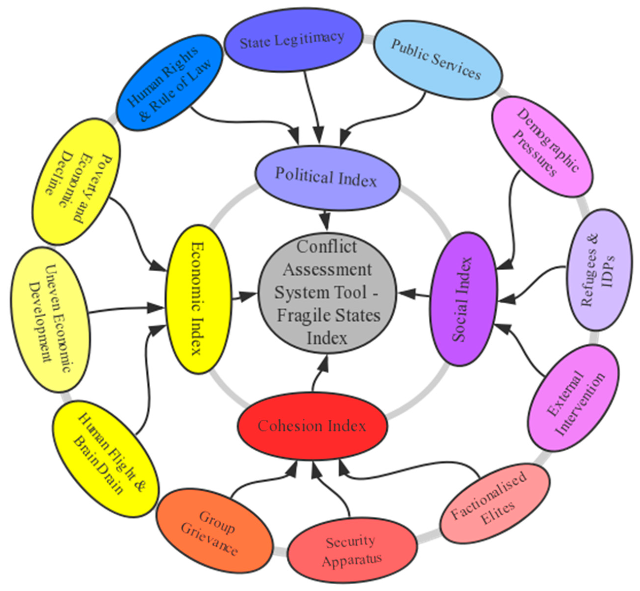
CAST is an excellent metric system to measure the fragility of states, which consists of four second-level indexes: Cohesion Index (CI), Economic Index (EI), Political Index (PI), and Social Index (SI). However, as lots of literature has mentioned that the climate change may further aggravate the state fragility, we introduce a new second-level index, Climate Change Performance Index (CCPI), to build FSMS based on the CAST.

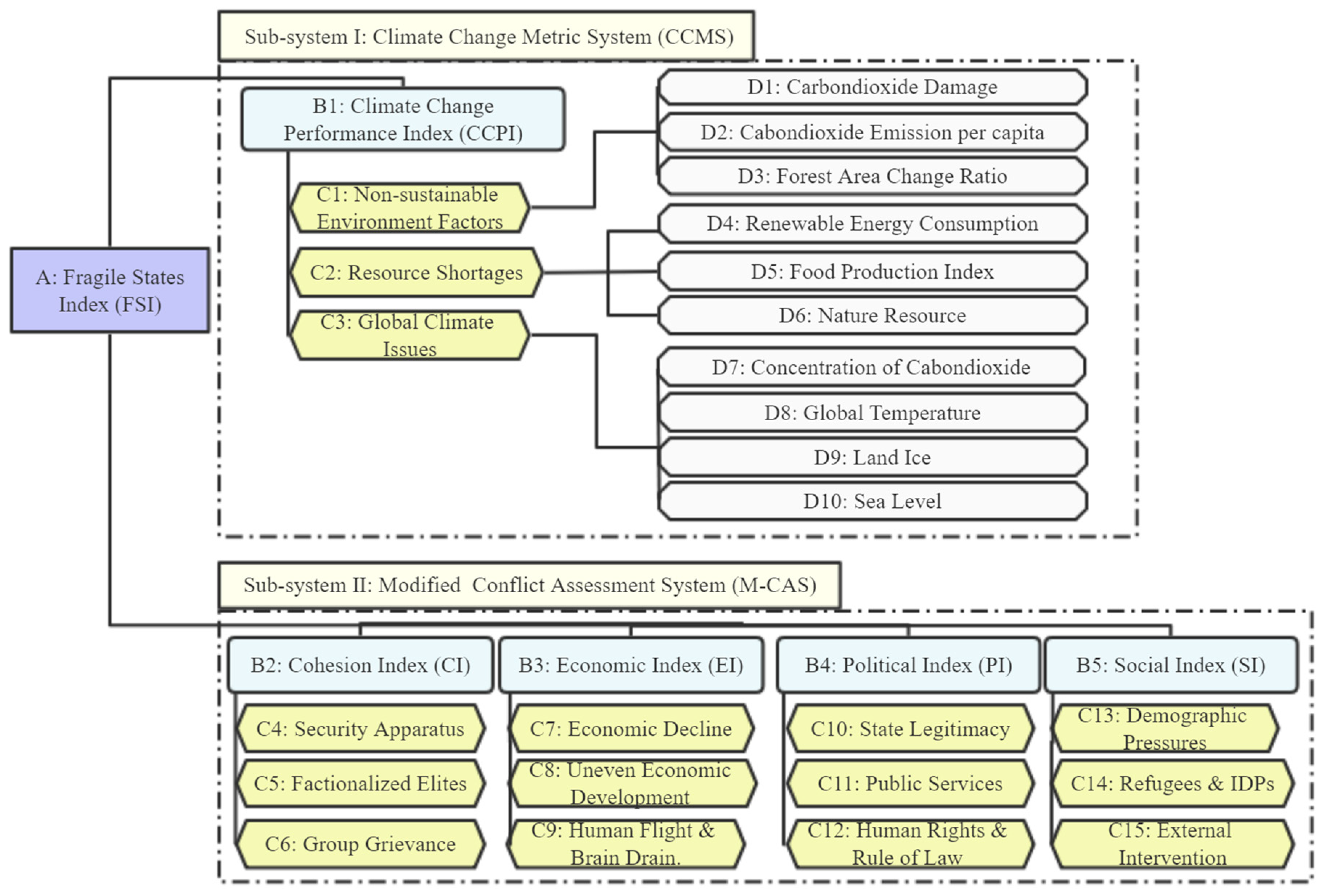
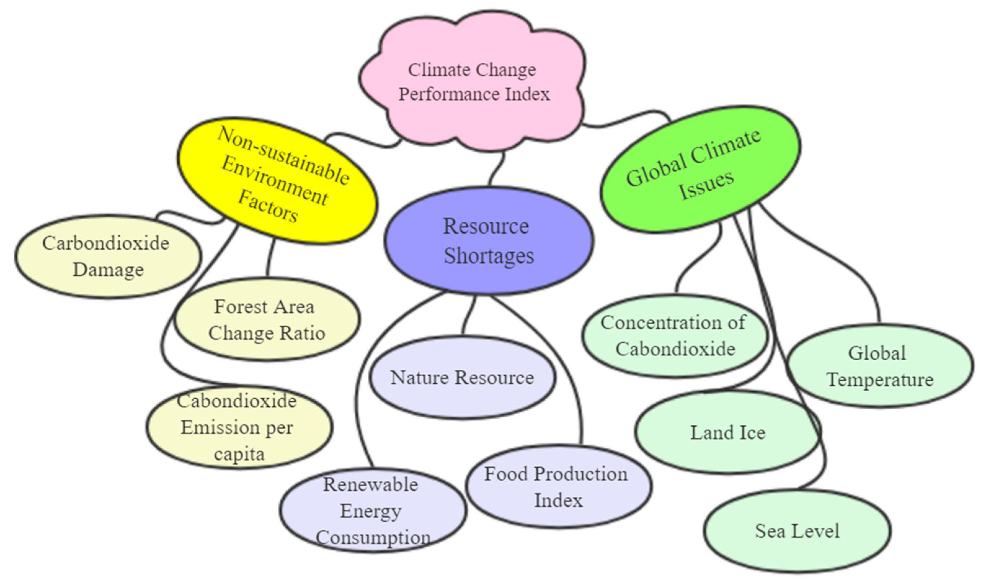
In our paper, we establish a four-layer Metric System. The first-level index is the Fragile States Index (FSI) and the second-level indexes are CI, EI, PI, SI and CCPI. As for the third-indexes, on the one hand, we adopt the index system structure of the CAST. Therefore, the sub-indexes of CI are Security Apparatus, Factionalized Elites and Group Grievance, and those of EI are respectively Economic Decline, Uneven Economic Development and Human Flight & Brain Drain. Similarly, as for PI, the sub-indexes are State Legitimacy, Public Services and Human Rights & Rule of Law and as for SI, the sub-indexes are Demographic Pressures, Refugees and IDPs and External Intervention. On the other hand, for the new second-level index CCPI, considering the structural unity of the M-CAS system, we introduce three secondary indexes, of which two secondary indexes are regional indexes and one is a global index (because climate change has impacts on both regional and global dimensions. Here, we introduce three sub-indexes to measure it, including Resource Shortages (RS), Non-sustainable Environment Factors (NEF) and Global Climate Issues (GCI). The first two are regional indexes and the last one is a global index. As for the fourth-level indexes (bottom indexes), we regard them as the sub-indexes of third-level indexes under CCPI. In terms of RS, taking into account the different phenomena caused by natural resource shortages and data integrity, we introduce 3 indexes: Renewable Energy Consumption, Food Production Index, and Nature Resource. By analyzing so many Non-sustainable Environment Factors, we believe that the CO₂ emission and deforestation have significant impacts on state fragility. In terms of NEF, we introduce CO₂ Damage, CO₂ Emission per Capita and Forest Area Change Ratio. Distinguishingly, the last sub-index Global Climate Issues is a global index, which has equal influences on different countries. Among the phenomena caused by global climate change, the greenhouse effect, sea-level rise, and global glacial area reduction are three major results. The corresponding sub-indexes include the Global Concentration of CO₂, Global Temperature, Land Ice and Sea Level. Therefore, in terms of GCI, its Sub-indexes include Concentration of CO₂, Global Temperature, Land Ice and Sea Level.

The overview of our system is shown in Figure 1 and the description of indexes is shown in

Table 1. Description of each index.

Index Level	Index	Index Description & References
First-Level	Fragile State Index (FSI)-A	The index aiming to assess states’ vulnerability to conflict or collapse [44,45]
Second-Level	Climate Change Performance Index (CCPI)-B1	The index including factors in the climate field that could affect states’ vulnerability [44,46]
	Cohesion Index (CI)-B2	The strength of cohesion that could affect states’ vulnerability [44,46]
	Economic Index (EI)-B3	The index including factors in the economic field that could affect states’ vulnerability [44,46]
	Political Index (PI)-B4	The index including factors in the political field that could affect states’ vulnerability [44,46]
	Social Index (SI)-B5	The index including factors in the social field that could affect states’ vulnerability [44,46]
Third-Level	Non-sustainable Environment Factors (NEF)-C1	The relationship between the state’s vulnerability and its non-sustainable environmental practice [5,24]
	Resource Shortages (RS)-C2	The influence and impact of resource, particularly resource shortages [27,28]
	Global Climate Issues (GCI)-C3	Shocks of abnormal climate changes [23,25]
	Security Appratus-C4	The security threats to a state, such as bombings, attacks and war causalities, rebel movements, mutinies, coups, or terrorism [44]
	Factionalized Elites-C5	The fragmentation of state institutions along ethnic, class, clan, racial or religious lines, as well as and brinksmanship and gridlock between ruling elites. [44]
	Group Grievance-C6	Divisions and schisms among different groups in society—particularly divisions based on social or political characteristics [44]
	Economic Decline-C7	Factors related to economic decline within a country [44]
	Uneven Economic Development-C8	The inequality within the economy, irrespective of the actual performance of an economy [44]
	Human Flight & Brain Drain-C9	The economic impact of migration (for economic or political reasons) and the consequences this may have on a country’s development [44]
	State Legitimacy-C10	The representativeness and openness of government and its relationship with its citizenry. [44]
	Public Services-C11	refers to the presence of basic state functions that serve the people [44]
	Human Rights & Rule of Law-C12	The relationship between the state and its population as far as fundamental human rights are protected and freedoms are observed and respected [44]
	Demographic Pressure-C13	The pressures upon the state deriving from its own citizens or the environment around it [44]
	Refugees & IDPs-C14	The index measuring the pressure upon states caused by the forced migration of large communities as a result of social, political, environmental or other causes, measuring displacement within countries, as well as refugee flows into others [44]
	External Intervention-C15	The external influence and impact to the functioning—particularly security and economic—of a state [44]
Fourth-Level	CO2 Damage-D1	The index is estimated to be $20 per ton of carbon (the unit damage in 1995 U.S. dollars) times the number of tons of carbon emitted.
	CO2 Emission-D2	The index is composed of CO2 total emission excluding short-cycle biomass burning but including other biomass burning, all anthropogenic CH4 sources, N2O sources and F-gases [47]
	Forest Area Change-D3	The index represents the displacement of trees in natural or artificial forest for at least 5 m, whether the forest is productive or not, and excludes trees in agricultural production systems and trees in urban parks and gardens [48]
	Renewable Energy Consumption-D4	The share of renewable energy in total final energy consumption [49]
	Food Production Index-D5	Covering food crops that are considered edible and that contain nutrients. Coffee and tea are excluded because, although edible, they have no nutritive value [50]
	Nature Resource-D6	The sum of oil rents, natural gas rents, coal rents (hard and soft), mineral rents, and forest rents [51]
	Concentration of CO2-D7	Global carbon dioxide levels.
	Global Temperature-D8	Average global temperature
	Land Ice-D9	Existing iceberg area
	Sea Level-D10	Average worldwide sea levels

.

3.1.1. Sub-System I: Climate Change Metric System

In Climate Change Metric System (CCMS), Climate Change Performance Index (CCPI) is the center. Non-sustainable Environmental Practices (NEP), Global Climate Issues (GCI), Resource Shortages (RS) are three second-level indexes of CCPI. As for the third-level indexes, based on considerable amount of literature in the field of climate change and Fragile States Index, we choose three third-level indexes for each second-level index. The complete CCMS is shown in Figure 2.

3.1.2. Sub-System II: Modified Conflict Assessment System

CAST is an analytical framework proposed by the FFP to measure the vulnerability of states. It evaluates qualitative and quantitative data stepwise and finally obtains a score of a country’s fragility. The higher the score, the more vulnerable the states. The CAST is shown in Figure 3.

Though it is an excellent fragility metric system, there are also some shortcomings. The FFP uses 12 second-level indexes to calculate the FSI. Further, the FFP considers that different indexes have same contribution to the FSI. Therefore, it assigns the 12 indexes the same weight. However, when climate change factors are considered, the structure of the index system will change. To modify CAST, the original set of equal weight will no longer apply to our new system FSMS. Therefore, we will focus on calculating the weights of indexes.

3.2. Preparation for CCMS Based on GRA

3.2.1. Data Preprocessing

● Data Complement

The data of our indexes come from the World Bank Database, National Aeronautics and Space Administration, Climate Change Knowledge Portland and so on. Considering the integrity and effectiveness of the data, we select the data from 2007 to 2017. However, the data is incomplete. Therefore, we use linear prediction model to fill in the missing data.

● Data Normalization

Date normalization is necessary before establishing an excellent model. In original dataset that we obtain from various databases, there are both efficiency index and cost index.

To make uniform the types of indexes, we should turn all indexes into cost indexes. Therefore, before normalizing data, we firstly use transform function to turn efficiency indexes into cost indexes. The transform function is as follows:

$$x_{cost}=\frac{1}{x_{efficiency}}$$

(1)

In this formula, $x_{efficiency}$ is the efficiency index needed to be transformed, $x_{cost}$ is the cost index after transformation.

Next, we can normalize all cost indexes; the normalization function is as follows.

$$x^{\prime }=\frac{x_{\max }-x}{x_{\max }-x_{\min }}$$

(2)

where, $x_{\max }$ is the maximum value of the sample while $x_{\min }$ is the minimum value, $x$ is the index value before normalization while $x^{\prime }$ is the one after normalization.

After normalization, the value of indexes ranges from 0 to 1. To simplify paper, we further convert the value interval from [0, 1] to [1, 10]. The transform function is shown as follows.

$$x_{result}=9x^{\prime }+1.$$

(3)

In this formula, $x^{\prime }$ is the index value after normalization with an interval of [0, 1] and $x_{result}$ is the transformed result with an interval of [1, 10].

3.2.2. Third-Level Weights Calculation Based on GRA

We determine third-level weights by the Gray Relational Analysis (GRA). Steps of using GRA to obtain weights are as follows.

Step 1: Determine comparison matrix

We define the evaluation matrix $H_{m\times n}$, and introduce $h_j(i)$, which represents $i(i=1,2,\cdots ,m)$ bottom index of $j(j=1,2,\cdots ,n)$ country. Thus, the comparison sequences are shown as follows.

$$H_j=(h_j(1),h_j(2),\cdots ,h_j(m)).$$

Step 2: Arrange parameter sequence

The optimal value of the comparison sequence is used in the reference sequence,

$$H_0=(h_0(1),h_0(2),\cdots ,h_0(m)).$$

In this formula, $h_0(i)(i=1,2,\cdots ,m)$ is the corresponding optimal value of $h_j(i)(j=1,2,\cdots ,n)$.

Because the indexes are all cost-type indexes, we obtain the reference sequence,

$$H_0=(1,1,1,1,1,1,1,1,1).$$

Step 3: Calculate correlation between $H_j$ and $H_0$

The absolute difference of comparison sequence is calculated as follows.

$${\Delta }_j(i)=|h_0(i)-h_j(i)|(i=1,2,\cdots ,m;1\le j\le n).$$

(4)

We notify that ${\Delta }_j=({\Delta }_j(1),{\Delta }_j(2),\cdots ,\Delta (m))$ and name it as difference sequence. Then, we define the correlation of comparison sequence $H_j$ and reference sequence $H_0$, which is

$$r(H_0(i),H_j(i))=\frac{\underset{j}{\min }\underset{i}{\min }{\Delta }_j(i)+\alpha \underset{j}{\max }\underset{i}{\max }{\Delta }_j(i)}{{\Delta }_j(i)+\alpha \underset{j}{\max }\underset{i}{\max }{\Delta }_j(i)}.$$

(5)

Here, we set resolution coefficients $\alpha$ at 0.5.

Step 4: Calculate correlations.

Then we measure the gray correlation of $H_j$ and $H_0$. The formula is

$$r_i=\frac{1}{n}{\displaystyle \sum _{j=1}^{n}r(H_0(i),H_j(i))}(i=1,2,\cdots ,m).$$

(6)

The value of gray correlation indicates the weighting of second-level index in integrated index. According to above steps we calculate the correlation matrix from 2007 to 2017.

Step 5: Calculate weights.

As for a certain year, the weight of an index is

$$w_i=\frac{r_i}{{\displaystyle \sum _{k=1}^m{r}_k}}i=1,2,\cdots ,m.$$

(7)

Finally, we calculate the 11-year average of weights and get the final weight of a specific index.

Employing the Gray Relational Analysis, we can obtain the weights of third-level indexes. They are shown in

Table 2. Third-level weights of CCMS.

Second-Level Index of CCMS-C	Third-Level Index of CCMS-D	Weight
		${\mathit{w}}_{\mathit{i}}$	${\mathit{w}}_{\mathit{i}\mathit{j}}$
Non-sustainable Environment Factors (NEF)-C1	CO2 Damage-D1	1	0.2745
	CO2 Emission-D2		0.2752
	Forest Area Change-D3		0.4503
Resource Shortage (RS)-C2	Renewable Energy Consumption-D4	1	0.3253
	Food Production Index-D5		0.2692
	Nature Resource-D6		0.4055
Global Climate Issues (GCI)-C3	Concentration of CO2-D7	1	0.2227
	Global Temperature-D8		0.2726
	Land Ice-D9		0.2157
	Sea Level-D10		0.2890

.

As we can see in Table 2, in terms of NEF, Forest Area Change weighs most. The weight of it is 0.4503. As for RS, Nature Resource contributes most with a weight 0.4055. However, when it comes to GCI, we can find that the weight of four sub-indexes of it are all closed to 0.25, which proves that four sub-indexes have almost the same contribution to the second-level index GCI.

3.3. Sub-System I: CCMS

3.3.1. Method I: Gray Relational Analysis

When it comes to the weights of second-level indexes in CCMS, we firstly use the GRA to calculate weights. Results are shown in

Table 3. Second-Level Weights of CCMS (GRA).

First-Level Index of CCMS-B	Second-Level Index of CCMS-C	Weight
		${\mathit{w}}_{\mathit{i}}$	${\mathit{w}}_{\mathit{i}\mathit{j}}$
Climate Change Performance Index (CCPI)-B1	Non-sustainable Environment Factors (NEF)-C1	1	0.2799
	Resource Shortage (RS)-C2		0.4182
	Global Climate Issues (GCI)-C3		0.3019

.

In Table 3, RS contribute the most to CCPI, and NEF makes the minimal contribution. To improve the scientificity of our system, we introduce the Entropy Method into our model. Combining GRA and the Entropy Method, we will obtain more accurate and reasonable results.

3.3.2. Method II: Entropy Method

Entropy is a method of measuring the disorder degree of a system. In the information theory, entropy is also used to measure the degree of dispersion [14]. It is believed that a greater dispersed index has a greater impact on results.

The key of Entropy Method is to quantify the information of unevaluated units. Steps of the Entropy Method are as follows:

Step 1: Calculate weights and entropy value.

Calculate the proportion of country $j$ among all second-level indexes:

$${p^{\prime }}_{zj}=\frac{{h^{\prime }}_j(\mathrm{z})}{{\displaystyle \sum _{j=1}^n{h^{\prime }}_j(\mathrm{z})}}\mathrm{z}=1,2,\cdots ,p;j=1,2,\cdots ,n.$$

(8)

Then we calculate the entropy value of the index $z$:

$$e_z=-k{\displaystyle \sum _{j=1}^n{p^{\prime }}_{zj}\ln {p^{\prime }}_{zj}}\hspace{1em}z=1,2,\cdots ,p.$$

(9)

The adjustment coefficient $k$ satisfies $k=\frac{1}{lnp}>0$.

Step 2: Calculate different coefficients.

We define different coefficient as $g_z=\frac{1-e_z}{9-E_e}$. Among them, $E_e={\displaystyle \sum _{z=1}^p{e}_z}$. In addition, coefficients’ range is $0\le g_z\le 1$, which satisfies ${\displaystyle \sum _{z=1}^p{g}_z}=1$.

Step 3: Calculate weights.

For a third-level index $z$, its calculation equation is

$$w_{z-e}=\frac{g_z}{{\displaystyle \sum _{z=1}^p{g}_z}}=g_z,z=1,2,\cdots ,p.$$

(10)

The weight of each index is an average weight from 2007 to 2017, 11 years as total. We do not have enough space to give a comprehensive display of the Entropy Method, so we just show the results in the next section.

The Entropy Method is in line with our expectation, which shows a large degree of dispersion and proves what we have obtained. In next section, we will discuss about the combined method, GRA-Entropy method.

3.3.3. Methods Combination: GRA-Entropy Method

(1) Combined Model

To combine the Gray Relational Analysis and the Entropy Method together, we introduce a parameter $\alpha$. If $\alpha =1$, then the weights calculated by these two methods weigh equally; if $\alpha >1$, then the Entropy Method will play a more important role in the weight calculation; if $\alpha <1$, then the Gray Relational Analysis outweigh the EM. The calculation function is as follows.

$$w_f=\frac{w_{f-g}+\alpha w_{f-e}}{1+\alpha }.$$

(11)

In this formula, $w_f$ is the weight of an index $f$, $w_{f-g}$ and $w_{f-e}$ is respectively the weights calculated by the Gray Relational Analysis and the Entropy Method. We introduce the Golden Ratio to make a decision and set the parameter $\frac{\alpha }{1+\alpha }=0.618$, that is $\alpha \approx 1.618$, which means we emphasize the importance of the Entropy Method.

(2) Results Analysis

Two approaches of measuring weights are combined through the parameter $\alpha$. The calculation results are shown in

Table 4. Second-Level Weights of CCMS (GRA-Entropy).

First-Level Index of CCMS-B	Second-Level Index of CCMS-C	Weight
		${\mathit{w}}_{\mathit{i}}$	${\mathit{w}}_{\mathit{i}\mathit{j}}$
Climate Change Performance Index (CCPI)-B1	Non-sustainable Environment Factors (NEF)-C1	1	0.2038
	Resource Shortage (RS)-C2		0.6096
	Global Climate Issues (GCI)-C3		0.1866

.

In Table 4, we can find that RS contribute the most to CCPI, and GCI makes the minimal contribution, which meets with our expectation that GCI is an index which has overall impact on every country in the world, so it has the minimal contribution to CCPI.

Based on the weights calculated above, we can obtain the value of CCPI results from 2007 to 2017. For well layout, we only show partial results in

Table 5. CCPI results.

Country	2007	2008	2009	2010	2011	2012	2013	2014	2015	2016	2017
Finland	4.839	4.404	4.952	3.967	3.961	4.054	3.888	4.089	4.434	4.185	4.763
Switzerland	4.734	4.268	4.887	3.995	3.949	3.971	3.675	3.883	4.144	3.863	4.418
Norway	5.703	5.267	5.797	4.783	4.671	4.824	4.615	4.781	4.955	4.572	4.989
Denmark	4.629	4.245	4.818	3.918	3.935	4.036	3.733	3.995	4.251	3.974	4.533
Australia	4.401	4.058	4.62	3.741	3.637	3.755	3.546	3.686	3.878	3.565	4.072
Ireland	4.358	3.735	4.306	3.546	3.508	3.445	3.268	3.445	3.779	3.533	4.121
Canada	4.675	4.433	4.845	3.95	3.802	3.905	3.738	3.826	4.053	3.761	4.279
New Zealand	4.916	4.429	5.038	4.203	4.082	4.171	3.908	4.152	4.355	4.082	4.614
Luxembourg	4.078	3.751	4.315	3.264	3.162	3.188	3.045	3.345	3.711	3.526	4.156
Sweden	5.04	4.611	5.265	4.34	4.23	4.346	4.108	4.291	4.6	4.305	4.852
Netherlands	4.415	3.991	4.618	3.724	3.634	3.668	3.422	3.622	3.831	3.556	4.098
Germany	4.455	4.036	4.653	3.746	3.651	3.718	3.458	3.697	3.95	3.699	4.266
Austria	4.89	4.518	5.05	4.167	4.101	4.127	3.886	4.121	4.398	4.141	4.707
Belgium	4.268	3.668	4.376	3.585	3.547	3.576	3.364	3.338	3.686	3.355	3.91
Portugal	4.664	4.283	4.956	4.169	3.95	3.978	3.862	4.002	4.36	4.121	4.714
United Kingdom	4.308	3.958	4.481	3.642	3.585	3.528	3.323	3.576	3.867	3.634	4.22
Slovenia	4.393	3.936	4.596	3.792	3.654	3.647	3.429	3.619	4.003	3.737	4.336
France	4.354	3.926	4.586	3.714	3.634	3.661	3.428	3.604	3.908	3.64	4.211
United States	4.374	3.964	4.536	3.649	3.503	3.555	3.361	3.555	3.786	3.533	4.085
Japan	4.356	3.891	4.446	3.543	3.403	3.467	3.212	3.334	3.657	3.365	3.934
South Africa	4.659	4.613	4.913	4.143	3.9	3.974	3.782	3.989	4.102	3.777	4.247
Thailand	5.061	4.554	5.096	4.17	4.096	4.311	4.007	4.187	4.275	3.941	4.413
Poland	4.383	3.955	4.587	3.648	3.544	3.671	3.449	3.697	3.937	3.693	4.252

Notes: the data is the result of CCPI, varying from 1.0 to 10.0. Lower value means the Climate Change brings less impact on the fragility of corresponding country.

.

3.4. Sub-System II: M-CAS Based on the GRA-Entropy Method

As we can see in the establishing process of sub-system I, the result of the GRA-Entropy Method is more reasonable than that of the GRA method. Therefore, we select the former method to establish the sub-system II. As the steps above, we can obtain the results shown in

Table 6. Second-Level Weights of M-CAS (GRA-Entropy).

Cohesion Index (CI)-B2	Weight	Economy Index (EI)-B3	Weight
Security Apparatus-C4	0.3675	Economy-C7	0.3200
Factionalized Elites-C5	0.3509	Economic Inequality-C8	0.2986
Group Grievance-C6	0.2816	Human Flight & Brain Drain-C9	0.3814
Policy Index (PI)-B4	Weight	Society Index (SI)-B5	Weight
State Legitimacy-C10	0.3365	Demographic Pressures-C13	0.2897
Public Services-C11	0.3341	Refugees & IDPs-C14	0.3672
Human Rights-C12	0.3294	External Intervention-C15	0.3431

.

The weights calculated by the GRA-Entropy method are clearly more accurate than those only by the GRA or the Entropy Method. The dispersion of weights varies with the structure of secondary indexes, which reflects the relevance of the indexes.

Due to the limited length of our paper, we are not going to show the results of CI, EI, PI and SI. As the method of calculating them is the same as that of CCPI, we are not going to show the results of the four indexes. In the next section, we introduce a new method to combine the two sub-systems.

3.5. Success of FSMS Based on Variable Weight Function

Data and cases can prove that climate change does have a significant impact on state fragility. The connection between them is indirect but notable. More importantly, this connection is in line with our understanding. When climate changes become extreme, giving rise to problems such as abnormal precipitation or frequent natural disasters caused by global warming, the basic resources on which people depend will inevitably reduce, and social order may be affected [23]. If the government does not take proper measures, the development of society may be affected. When resources are scarce, people will compete for resources and conflicts will occur. Poverty may be further aggravated.

This influence might be far-reaching and wide-ranging. Efforts made to improve the poor situation may have impacts on the economy, and poor conditions may have a negative influence on social stability and economic development. At the same time, the credibility of the government may be affected by people’s dissatisfaction and further affect the stability of the country.

What needs to be pointed out is that climate change will make the already fragile situation even worse. This is more clearly reflected in climate change and resources shortage in developing countries. When climate change acts as a “threat multiplier”, countries that were at risk of instability may be caught in a vicious cycle. [32] This also explains why more examples of climate change affecting state fragility appear in relatively backward continent, Africa.

The link between climate change and national fragility shows that we should include climate factors in the evaluation system. In addition, we will set a variable weight function to measure the impact of climate change on state fragility because climate change takes effect only when a country is vulnerable enough [5]. We believe the weight, which is the contribution of CCPI to FSI, will abruptly increase when FSI is great enough (the country is vulnerable enough). To combine sub-system I and sub-system II, we introduce variable weight function method to determine the weights of second-level indexes of FSMS, including CI, EI, PI, SI and CCPI.

3.5.1. Introduction of Variable Weight Function Method

In our paper, we introduce variable weight functions based on the Logistic Function. Logistic Function is a common “S” shape function. Its general form is

$$f(x)=\frac{L}{1+e^{-k(x-x_0)}}.$$

where $L$ is the maximum value on the curve, $k$ is the slope of the curve, $x_0$ is the abscissa of the symmetry point. The curve of standard logistic sigmoid function is shown in Figure 4.

Considering the characteristic of second-level weights of FSMS, we set following principles to determine the variable weight functions:

Principle 1: variable weight functions of five second-level indexes have the same form.

Principle 2: variable weight function belongs to piecewise functions. The boundary point of the function is a threshold value of CCPI value. When the value of the independent variable is less than the threshold, the corresponding weight increases slowly. When it exceeds the threshold, the weight will increase abruptly. In the functions, the independent variable is the value of CCPI and its corresponding index; the dependent variable is the weight of corresponding index.

Principle 3: In this principle, there is also a threshold value for CCPI. Only when the value of the independent variable is greater than the threshold and the value of CCPI is greater than the CCPI threshold, will the dependent variable increase in a rather rapid state. However, if the value of the independent variable is greater than the threshold, but the value of CCPI is less than the CCPI threshold, the dependent variable will increase in a relatively slow rate.

Based on the theory of Logistic Function and two principles listed above, we introduce variable weight function as following forms:

$$w_f=\{\begin{array}{ll}t\left[1-\frac{L}{1+e^{-k(c_f-c_f^0)}}\right]& 1\le c_f<c_{threshold}\\ t{e}^{m_f(c_{climate}-c_{climate}^0)}\left[1-\frac{L}{1+e^{-k(c_f-c_f^0)}}\right]& c_{threshold}\le c_f\le 10\end{array}$$

(12)

In this formula, there are following variables.

Independent variables: $c_f$, the value of index $f$ (CI, EI, PI or SI); $c_{climate}$, the value of index CCPI.

Dependent variables: $w_f$, the weight of index $f$ (CI, EI, PI or SI).

Parameters:

$t$, the maximum weight a secondary index can have, here finally we set it at 0.225;

$L$, the supreme value of the Logistics Function, here we set it at 1;

$k$, the gradient parameter of the Logistics Function, here we set it at 1;

$c_f^0$, the abscissa of the symmetrical point of an index in the Logistic Function;

$m_f$, the amplification factor which reflects the multiple effects of the CCPI on the index $f$;

$c_{climate}^0$, the boundary point of CCPI, here we set it at 5;

$c_{threshold}$, the boundary point of a variable function, here we set it at 6.5.

To establish various function for different indexes (CI, EI, PI and SI), we set a series of parameters for them on the basis of characteristic of different indexes. For lack of space, we only show the result of our analysis on variable weight functions at

Table 7. Variable Weight Functions of Different Indexes.

Index	Variable Weight Function
Cohesion Index (CI)	$w_{CI}=\{\begin{array}{cc}0.225\left[1-\frac{1}{1+e^{-(c_{CI}-4)}}\right]\hfill & \hfill 1\le c_{CI}<6.5\\ 0.225e^{0.2243(c_{CCPI}-5)}\left[1-\frac{1}{1+e^{-(c_{CI}-4)}}\right]\hfill & \hfill 6.5\le c_{CI}\le 10\end{array}$
Economic Index (EI)	$w_{EI}=\{\begin{array}{cc}0.225\left[1-\frac{1}{1+e^{-(c_{EI}-4.5)}}\right]\hfill & \hfill 1\le c_{EI}<6.5\\ 0.225e^{0.3919(c_{CCPI}-5)}\left[1-\frac{1}{1+e^{-(c_{EI}-4.5)}}\right]\hfill & \hfill 6.5\le c_{EI}\le 10\end{array}$
Political Index (PI)	$w_{PI}=\{\begin{array}{cc}0.225\left[1-\frac{1}{1+e^{-(c_{PI}-5.5)}}\right]\hfill & \hfill 1\le c_{PI}<6.5\\ 0.225e^{0.3133(c_{CCPI}-5)}\left[1-\frac{1}{1+e^{-(c_{PI}-5.5)}}\right]\hfill & \hfill 6.5\le c_{PI}\le 10\end{array}$
Social Index (SI)	$w_{SI}=\{\begin{array}{cc}0.225\left[1-\frac{1}{1+e^{-(c_{SI}-6)}}\right]\hfill & \hfill 1\le c_{SI}<6.5\\ 0.225e^{0.1215(c_{CCPI}-5)}\left[1-\frac{1}{1+e^{-(c_{SI}-6)}}\right]\hfill & \hfill 6.5\le c_{SI}\le 10\end{array}$

.

In addition, the weight of CCPI is calculated as followed.

$$w_{CCPI}=1-w_{CI}-w_{EI}-w_{PI}-w_{SI}.$$

(13)

Therefore, on the basis of weight of 5 second-level indexes (CI, EI, PI, SI and CCPI), we can easily calculate the value of first-level index, i.e., FSI.

$$FSI=W·C.$$

(14)

3.5.2. Result Analysis of FSMS

Based on the Fragile State Metric System (FSMS) established above, we calculate the FSI of 132 countries around the world (because lots of data for some countries is missing, we only select 132 countries to calculate the results), which vary from 2007 to 2017. Moreover, we obtain the FSI ranking from 2007 to 2017 of the 132 selected countries. Due to lack of space, we only show partial results in

Table 8. Top 5 Most Stable Countries from 2007 to 2017.

	Rank	1	2	3	4	5
Year
2007		Norway	Finland	Ireland	Sweden	Switzerland
2008		Norway	Finland	Ireland	Switzerland	Sweden
2009		Finland	Norway	Ireland	Switzerland	Sweden
2010		Finland	Norway	Switzerland	Sweden	Ireland
2011		Finland	Norway	Switzerland	Sweden	Denmark
2012		Finland	Sweden	Denmark	Switzerland	Luxembourg
2013		Finland	Sweden	Switzerland	Denmark	Luxembourg
2014		Finland	Sweden	Denmark	Switzerland	Luxembourg
2015		Finland	Sweden	Denmark	Luxembourg	Norway
2016		Finland	Denmark	New Zealand	Switzerland	Australia
2017		Finland	Switzerland	Norway	Denmark	Australia

. The complete results are shown in Appendix A.

Due to lack of space, we only analyze the FSI results in 2017 as an example. As we can see in

Table 9. FSI & Ranking results (partial countries).

Country	2007	2008	2009	2010	2011	2012	2013	2014	2015	2016	2017
Finland	1.955 (2)	1.889 (2)	2.022 (1)	1.905 (1)	1.942 (1)	1.98 (1)	1.807 (1)	1.881 (1)	1.859 (1)	1.902 (1)	1.982 (1)
Switzerland	2.045 (5)	1.989 (4)	2.14 (4)	2.062 (3)	2.172 (3)	2.196 (4)	2.004 (3)	2.176 (4)	2.133 (6)	2.052 (4)	2.083 (2)
Norway	1.939 (1)	1.861 (1)	2.046 (2)	1.953 (2)	2.079 (2)	2.35 (6)	2.128 (7)	2.279 (7)	2.12 (5)	2.108 (7)	2.114 (4)
Denmark	2.197 (7)	2.085 (6)	2.291 (6)	2.145 (6)	2.223 (4)	2.18 (3)	2.047 (4)	2.148 (3)	2.075 (3)	2.028 (2)	2.115 (3)
Australia	2.205 (8)	2.262 (8)	2.447 (8)	2.426 (9)	2.484 (9)	2.575 (12)	2.265 (9)	2.349 (9)	2.233 (8)	2.059 (5)	2.124 (5)
Ireland	1.975 (3)	1.916 (3)	2.128 (3)	2.081 (4)	2.296 (6)	2.369 (7)	2.215 (8)	2.33 (8)	2.278 (9)	2.089 (6)	2.175 (6)
Canada	2.424 (10)	2.468 (11)	2.647 (12)	2.521 (12)	2.492 (11)	2.441 (9)	2.363 (10)	2.485 (10)	2.382 (10)	2.198 (8)	2.179 (7)
New Zealand	2.116 (6)	2.101 (7)	2.339 (7)	2.242 (7)	2.302 (7)	2.365 (8)	2.116 (6)	2.252 (6)	2.166 (7)	2.037 (3)	2.219 (8)
Luxembourg	2.572 (12)	2.508 (12)	2.573 (10)	2.401 (8)	2.315 (8)	2.267 (5)	2.095 (5)	2.231 (5)	2.092 (4)	2.222 (9)	2.255 (9)
Sweden	2.042 (4)	2.023 (5)	2.175 (5)	2.076 (5)	2.22 (5)	2.122 (2)	1.963 (2)	2.12 (2)	2.057 (2)	2.222 (10)	2.266 (10)
Netherlands	2.644 (14)	2.465 (10)	2.548 (9)	2.482 (11)	2.514 (12)	2.506 (10)	2.374 (11)	2.532 (11)	2.427 (12)	2.506 (12)	2.531 (11)
Germany	3.399 (23)	3.231 (20)	3.277 (20)	3.034 (19)	2.927 (18)	2.797 (13)	2.593 (13)	2.697 (13)	2.542 (13)	2.558 (14)	2.612 (12)
Austria	2.497 (11)	2.435 (9)	2.649 (11)	2.484 (10)	2.494 (10)	2.517 (11)	2.43 (12)	2.587 (12)	2.433 (11)	2.543 (13)	2.643 (13)
Belgium	2.359 (9)	2.53 (13)	2.998 (14)	2.751 (14)	2.907 (16)	2.881 (15)	2.658 (14)	2.723 (14)	2.663 (14)	2.507 (11)	2.735 (14)
Portugal	2.978 (15)	2.866 (15)	3.068 (16)	2.947 (16)	2.858 (14)	2.988 (18)	2.853 (19)	2.933 (17)	2.74 (15)	2.667 (15)	2.762 (15)
United Kingdom	3.07 (18)	2.911 (17)	3.049 (15)	2.925 (15)	2.923 (17)	3.004 (19)	2.803 (17)	2.93 (18)	2.906 (18)	2.778 (16)	2.931 (16)
Slovenia	3.308 (21)	3.182 (19)	3.26 (19)	3.057 (20)	3.012 (20)	2.909 (16)	2.744 (15)	2.809 (15)	2.797 (16)	2.95 (20)	2.95 (17)
France	3.024 (16)	2.981 (18)	3.151 (18)	2.958 (17)	2.885 (15)	2.866 (14)	2.755 (16)	2.935 (16)	2.902 (17)	2.923 (18)	2.958 (18)
United States	3.028 (17)	2.886 (16)	3.087 (17)	3.008 (18)	2.941 (19)	2.962 (17)	2.827 (18)	3.003 (19)	3.03 (19)	2.884 (17)	3.072 (19)
Japan	2.616 (13)	2.643 (14)	2.849 (13)	2.714 (13)	2.671 (13)	3.395 (21)	2.975 (20)	3.033 (20)	3.07 (20)	2.951 (19)	3.19 (20)
South Africa	4.608 (43)	4.772 (65)	5.117 (58)	4.651 (71)	4.523 (72)	4.568 (68)	4.453 (69)	4.57 (70)	4.632 (66)	4.438 (71)	4.715 (64)
Thailand	5.28 (76)	4.917 (72)	5.333 (69)	4.571 (67)	4.488 (67)	4.661 (73)	4.414 (67)	4.529 (67)	4.55 (60)	4.28 (56)	4.637 (60)
Poland	3.919 (29)	3.777 (28)	4.128 (29)	3.756 (31)	3.67 (28)	3.596 (25)	3.366 (22)	3.501 (25)	3.405 (22)	3.436 (24)	3.574 (25)

Notes: The format of data is: FSI (Ranking).

, among the top 20 most stable counties, there are 15 countries located in Europe, including 6 Western European countries (Ireland, Luxembourg, Netherlands, Belgium, United Kingdom and France), 4 Northern European countries (Finland, Norway, Denmark and Sweden), 3 Central European countries (Switzerland, Germany and Austria) and 2 Southern European countries (Portugal and Slovenia). There are 2 countries in Oceania (Australia and New Zealand), 2 in North America (Canada and United States) and 1 in Eastern Asia (Japan). Therefore, we can easily find that in the top 20 most stable countries in 2017, 75% are located in Europe, and the remaining 15% are in Oceania, North America and Eastern Asia.

Similar to the above analysis of FSI results in 2017, we can analyze the 2007–2017 FSI calculation results in Appendix A. The analysis of the results shows that in 2007–2017, the five most stable countries each year are the Nordic countries (The FSL result is in an ascending order, which means that the more stable the countries has smaller FSI values). Table 8 below analyzes the top 5 most stable countries in 2007–2017 based on the FSMS model.

Table 8 shows that based on the FSMMS model we constructed, from 2007 to 2017, among the 132 countries to be tested, the 5 most stable countries are the Nordic countries. The five typical countries are Finland, Norway, Switzerland, Sweden and Denmark. Across these 10 years, these five countries have always ranked among the top five most stable and sustainable countries.

In fact, the Nordic countries, such as Finland, Norway, Sweden and Denmark, are all recognized as the most sustainable countries; therefore the levels of their fragility are also the lowest among those of all countries. In 2018, the UN reported that the happiest country in the world is Finland in the World Happiness Report 2018, [52], followed by Norway and Denmark. At the same time, in the 2017 World Happiness Report 2017, the happiest country is Norway, [53], followed by Denmark, Iceland and Switzerland. Similarly, the Nordic countries have long been the most sustainable countries in the world. Therefore, the five most stable countries pointed out in our model analysis results—Finland, Norway, Switzerland, Sweden and Denmark—are indeed the most stable countries in the world currently. At the same time, our model shows that even in the case of climate change, the fragility levels of these countries are still low, indicating that their sustainability and stability are quite good.

3.6. Robustness Analysis of FSMS

3.6.1. Impact of $\alpha$

In GRA-Entropy method mentioned above, we introduce a parameter $\alpha$ to combine the GRA and the Entropy Method. Here, we want to discuss the impact of $\alpha$, testifying its effects on our FSMS model. In the previous part of our paper, we set $\alpha =1.618$. Then we revalue the weight at $\frac{\alpha }{1+\alpha }=0.25$ and $\frac{\alpha }{1+\alpha }=0.5$, which means that $\alpha =0.3$ and $\alpha =1$. For the lack of space, we only select 6 representative countries. The result is shown in Figure 5.

In Figure 5, we can find that when $\alpha$ is set at different value, the ranking and FSI value of the six countries only change a little, which means that the value of $\alpha$ has little effect on the result of FSMS model. Therefore, FSMS model is a rather robust model.

3.6.2. Impact of $m_f$ and $c_f^0$

$m_f$ and $c_f^0$ are used in the variable weight function, which reflect the weight of the four indicators, except the CCPI, on the FSI. In the previous section, $C_0^0=[\begin{array}{cccc}4.5,& 5,& 5.5,& 6\end{array}]$ and $M_0=[\begin{array}{cccc}0.2243,& 0.3919,& 0.3133,& 0.1215\end{array}]$. Here we take two vectors as follows.

$$C_1^0=[\begin{array}{cccc}4,& 4.5,& 5,& 5.5\end{array}], M_1=[\begin{array}{cccc}0.3133,& 0.4621,& 0.3919,& 0.2243\end{array}]$$

$$C_2^0=[\begin{array}{cccc}5,& 5.5,& 6,& 6.5\end{array}], M_2=[\begin{array}{cccc}0.1215,& 0.3133,& 0.2243,& 0.0635\end{array}]$$

For the lack of space, we take UK as an example and calculate the FSI of different parameters as is shown in Figure 6.

As can be seen in Figure 6, the greater the $m_f$ is, the greater the weight of CCPI is, which means that when CCPI contribute more to FSI, the other second-level indexes (CI, EI, PI and SI) contribute less. Meanwhile, the greater the $c_f^0$ is, the less the weight of CCPI is, which means that when CCPI contribute less to FSI, the other second-level indexes (CI, EI, PI and SI) contribute more. This phenomenon is in consonance with our expectation in the previous part. Therefore, the impact of $m_f$ and $c_f^0$ meets with our expectation, which also shows that our model is a robust and controllable model.

4. Application of the FSMS with Pareto Optimum

4.1. Pareto Optimum

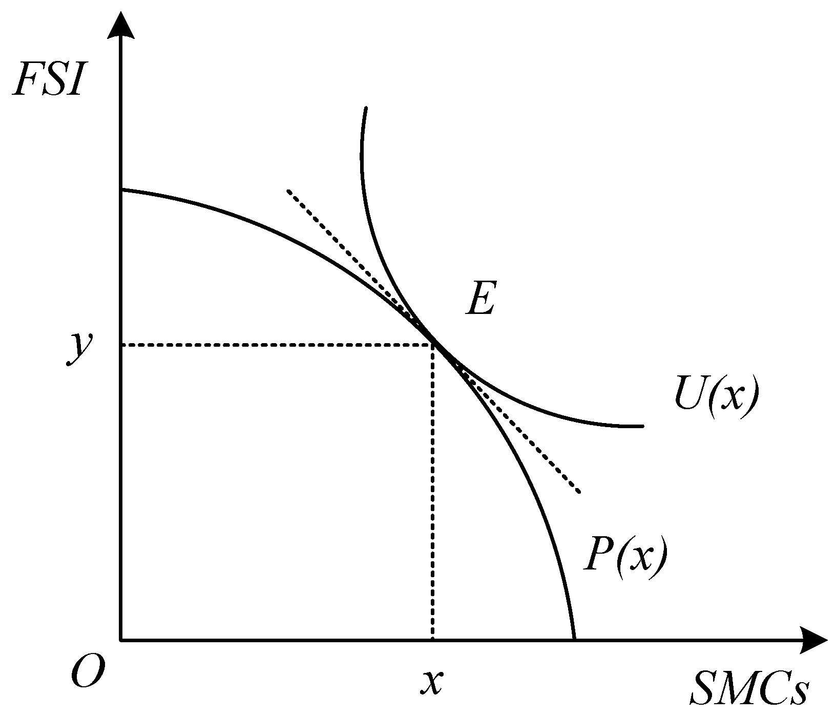
Pareto equilibrium is a method to represent the optimal state of social exchange. Assuming that there is a fixed group of people and allocable resources, we cannot make any person’s situation better without making any other’s worse. Here we employ an economic model that consists of two parts, production possibility frontier (PPF) and utility function. The production possibility frontier is a curve which can show all possible combinations of two goods, and the utility function is a kind of indifference curve that all combinations on it have the same utility.

We assume that there are two kinds of goods, state insurance and national stability (we assume that it can be bought). They are purchased by a state leader using a kind of limited resource, the state revenue. A state leader should make a choice of the quantities of both goods. We use two variables to substitute these “goods”, which are the state maintenance costs (SMCs) and the fragile state index (FSI). Therefore, we can introduce them in a decision-making model.

In Figure 7, E is the tangent point of the PPF and the Utility Function. Convex form of production possibility frontier can well describe the characteristics of the SMCs and the FSI. The Pareto Optimum is achieved when the PPF is tangent to the utility curve. We define $U(x)$ as utility function and $P(x)$ as production boundary. The original state is marked as $(x_0,y_0)$ and then we obtain these equations.

$$U(x_0)=P(x_0),$$

$$\frac{\partial U(x_0)}{\partial x}=\frac{\partial P(x_0)}{\partial x}.$$

4.2. State Maintenance Costs Analysis Based on FSMS and Pareto Optimum

If a state encounters a big shock such as destructive disasters or a war, then the production possibility frontier will shift outward when the cost of maintaining the nation stability increases because of the adverse change; when the national economy is well developed and society is stable enough, the production possibility frontier will shift toward the left because of the improvement in many aspects. It is noted that the utility function is not a single curve, but a cluster of curves. The Pareto Optimum will change with different production possibility frontiers. $(x_1,y_1)$ is marked as the latter state after the big shock. The fragile level changes from $y_0$ to $y_1$, and we established the following equations,

$$SMCs=AutonomousRecovery+InternationalIntervention,$$

$$AutonomousRecovery=x_1-x_0$$

In these formulas, Autonomous Recovery is the domestic part of SMCs; International Intervention is the external assistance.

Obviously, it is difficult for a country to recover from a destructive disaster or a war without the international intervention. In our model, the external assistance can be expressed as

$$InternationalIntervention=\Delta a-\Delta x$$

We are going to discuss the shape of the utility curve further. For a developed country, its ability to withstand and resolve shocks is better than the developing country. These countries can afford higher costs of internal stability with less need for external assistance. Thus, developed counties’ utility curve is closer to the X-axis; developing countries’ utility curve is closer to the Y-axis.

Without extra intervention, the costs of maintaining stability and the Fragile State Index are balanced in the long run. $E_0:(x_0,y_0)$ is the initial equilibrium point.

The intervention makes the SMCs reduce $\Delta \alpha$ while the production possibility frontier shifts from $P_0(x)$ to $P_1(x)$. As is shown in Figure 8, the Utility is reduced to $U_1$, which is a lower level. However, both the FSI and the SMCs are adverse variables and the final result is suitable for the empirical analysis.

5. Conclusions

State fragility reflects the overall condition of a country. Changes in politics, economy, culture, society, and the environment can make state fragility levels fluctuate. These factors have mutual effects on each other and have complex mechanisms of impact on fragility. Different countries have different reactions to the same level of shocks because of cultural and geographical factors. However, due to the complexity of these factors, we do not study the effect of cultural and geographical factors in this paper. Finally, this paper builds a metric system to assess state fragility. The system includes five dimensions: climate change, cohesion, economy, policy, and society, aiming at calculating the Fragile States Index of 132 states from 2007 to 2017. In the process of establishing the system, a new hybrid evaluation method GRA-Entropy method and variable weight function model are introduced to determine the weights of each index.

The FSMS includes two sub-systems. In the first sub-system, we establish the Climate Change Metric System, and in the second sub-system, we correct the CAS proposed by the FFP. The focus of our work lies in calculating the weights objectively. While calculating the weights of the second-level indexes, the Entropy Method is the supplement and improvement to the Gray Relational Analysis. As is shown in the calculated results, among the original 12 indicators from the Conflict Assessment System, Security Apparatus, Factionalized Elites, and Human Flight and Brain Drain are assigned greater weights, which is in line with reality. Then, we employ different variable weight functions to calculate the weights of the Climate Change Performance Index, the Cohesion Index, the Economic Index, the Political Index and the Social Index, so that we obtain the influence of climate change on other indexes. Judging from the Fragile State Index value results, stable countries are more likely to be in Europe, whereas the countries with worst conditions are mainly located in Africa and South America. More remarkably, wealthy and stable countries are still a minority. Besides, robustness analysis proves that the change of parameter values is relatively stable in our model, which demonstrates the accuracy of our model.

In summary, we introduce 5 different aspects to assess the fragility of states, in particular climate change, because we want to apply our model to solve practical problems. In Section 4, based on the FSMS, we use an economic theory of Production Possibility Frontier and Indifference Curve to measure the human intervention cost of the states when pursuing the stable development.

The index system proposed in this paper can help to comprehensively calculate the multi-dimensional fragility and reasonably evaluate and reflect the weights of different indicators. There is no appraisal system that can apply all the objects, but our work provides a new perspective for the evaluation of state fragility and the establishment of the indicator system.

Our model contains some fundamental limitations. The existing data is incomplete and some parameters are based on common sense. Despite this, the results are still accurate and robust. In brief, we hope that our methods in model establishment will offer reference for other relevant studies. In the future, this metric system can be applied to other different targets. For example, by changing the type of data, this model will work for other administrative divisions, such as cities, continents and so on.

References

- Wikipedia. Fragile State. Available online: https://en.wikipedia.org/wiki/Fragile_state (accessed on 8 April 2018).
- CPIA Public Sector Management and Institutions Cluster Average (1 = Low to 6 = High). Available online: https://data.worldbank.org/indicator/IQ.CPA.PUBS.XQ (accessed on 1 April 2018).
- Grimm, S.; Lemay-Hebert, N.; Nay, O. The Political Invention of Fragile States: The Power of Ideas; Routledge: Abingdon, UK, 2016; ISBN 978-1-317-62545-2. [Google Scholar]
- Miguel, E. Poverty and Witch Killing. Rev. Econ. Stud. 2005, 72, 1153–1172. [Google Scholar] [CrossRef]
- Mao, X. The Oretical Thinking on the Influence of Geographical Environment on Cultural Development. Tangdu J. 2001, 3, 55–61. Available online: http://kns.cnki.net/KCMS/detail/detail.aspx?dbcode=CJFQ&dbname=CJFD2001&filename=TDXK200103014&v=MDAwNDFyQ1VSTEtmWXVkdUZ5N2hWTHZBTVNuVFpiRzRIdERNckk5RVlJUjhlWDFMdXhZUzdEaDFUM3FUcldNMUY= (accessed on 8 April 2018).
- Li, Y. On Religious Electricity of the Affecting the Middle East Security. J. Jiangnan Soc. Univ. 2011, 3, 29–33. Available online: http://kns.cnki.net/KCMS/detail/detail.aspx?dbcode=CJFQ&dbname=CJFD2011&filename=JNSH201103007&uid=WEEvREcwSlJHSldRa1FhdXNXa0hIb3VTcVpjUnVNSzd4L0VTbWVnK0N0Zz0=$9A4hF_YAuvQ5obgVAqNKPCYcEjKensW4IQMovwHtwkF4VYPoHbKxJw!!&v=MDc5MjJQWVpyRzRIOURNckk5Rlk0UjhlWDFMdXhZUzdEaDFUM3FUcldNMUZyQ1VSTEtmWXVkdUZ5SGxXNy9CTHk= (accessed on 8 April 2018).
- Grimm, S. The European Union’s ambiguous concept of ‘state fragility’. Third World Q. 2014, 35, 252–267. [Google Scholar] [CrossRef]
- Nay, O. International Organisations and the Production of Hegemonic Knowledge: How the World Bank and the oecd helped invent the Fragile State Concept. Third World Q. 2014, 35, 210–231. [Google Scholar] [CrossRef]
- Nay, O. Fragile and failed states: Critical perspectives on conceptual hybrids. Int. Political Sci. Rev. 2013, 34, 326–341. [Google Scholar] [CrossRef]
- Grimm, S.; Lemay-Hébert, N.; Nay, O. ‘Fragile States’: Introducing a political concept. Third World Q. 2014, 35, 197–209. [Google Scholar] [CrossRef]
- Zoellick, R.B. Fragile States: Securing Development. Survival 2008, 50, 67–84. [Google Scholar] [CrossRef]
- Chauvet, L.; Collier, P.; Hoeffler, A. The Cost of Failing States and the Limits to Sovereignty, Wider Working Paper; UNU-WIDER: Helsinki, Finland, 2011. [Google Scholar]
- Patrick, S. Weak States and Global Threats: Assessing Evidence of Spillovers; The Center for Global Development: Washington, DC, USA, 2006. [Google Scholar]
- Hoeffler, A. Out of the Frying Pan into the Fire? Migration from Fragile States to Fragile States; OECD: Paris, France, 2013. [Google Scholar] [CrossRef]
- OECD. OECD Development Co-Operation Working Papers; OECD: Paris, France, 2017. [Google Scholar] [CrossRef]
- Africa Center for Strategic Studies. Africa’s Fragile States: Empowering Extremists, Exporting Terrorism; Africa Center for Strategic Studies: Washington, DC, USA, 2010. [Google Scholar]
- Goldstone, J.A. Pathways to State Failure. Confl. Manag. Peace Sci. 2008, 25, 285–296. [Google Scholar] [CrossRef]
- Boyanowsky, E. Violence and aggression in the heat of passion and in cold blood. The Ecs-TC syndrome. Int. J. Law Psychiatry 1999, 22, 257–271. [Google Scholar] [CrossRef]
- Homer-Dixon, T.F. Environment, Scarcity, and Violence; Princeton University Press: Princeton, NJ, USA, 2010; ISBN 978-1-4008-2299-7. [Google Scholar]
- Cooney, C.M. Managing the Risks of Extreme Weather: IPCC Special Report. Environ. Health Perspect. 2012, 120, a58. [Google Scholar] [CrossRef] [PubMed]
- Van Aalst, M.K. The impacts of climate change on the risk of natural disasters. Disasters 2006, 30, 5–18. [Google Scholar] [CrossRef] [PubMed]
- Schwartz, P.; Randall, D. An Abrupt Climate Change Scenario and Its Implications for United States National Security; California Inst of Tech Pasadena Jet Propulsion Lab: Pasadena, CA, USA, 2003.
- Barnett, J.; Adger, W.N. Climate change, human security and violent conflict. Political Geogr. 2007, 26, 639–655. [Google Scholar] [CrossRef]
- Theisen, O.M.; Gleditsch, N.P.; Buhaug, H. Is climate change a driver of armed conflict? Clim. Chang. 2013, 117, 613–625. [Google Scholar] [CrossRef]
- Anderson, C.A. Heat and Violence. Curr. Dir. Psychol. Sci. 2001, 10, 33–38. [Google Scholar] [CrossRef]
- Reuveny, R. Climate change-induced migration and violent conflict. Political Geogr. 2007, 26, 656–673. [Google Scholar] [CrossRef]
- Burke, M.B.; Miguel, E.; Satyanath, S.; Dykema, J.A.; Lobell, D.B. Warming increases the risk of civil war in Africa. PNAS 2009, 106, 20670–20674. [Google Scholar] [CrossRef] [PubMed]
- Lecoutere, E.; D’Exelle, B.; Van Campenhout, B. Who Engages in Water Scarcity Conflicts? A Field Experiment with Irrigators in Semi-Arid Africa; Social Science Research Network: Rochester, NY, USA, 2010. [Google Scholar]
- Mehlum, H.; Miguel, E.; Torvik, R. Poverty and crime in 19th century Germany. J. Urban Econ. 2006, 59, 370–388. [Google Scholar] [CrossRef]
- Hidalgo, F.D.; Naidu, S.; Nichter, S.; Richardson, N. Economic Determinants of Land Invasions. Rev. Econ. Stat. 2010, 92, 505–523. [Google Scholar] [CrossRef]
- Krakowka, A.R.; Heimel, N.; Galgano, F.A. Modeling Environmental Security in Sub-Saharan Africa. Geogr. Bull. 2012, 53, 21–38. [Google Scholar]
- New Security Beat. A New Climate for Peace: Taking Action on Climate and Fragility Risks (Report Launch); New Security Beat: Washington, DC, USA, 2015. [Google Scholar]
- Hoffman Worldwide. World Bank Develops New System to Measure Wealth of Nations—World Bank; Hoffman Worldwide: McLean, VA, USA, 1995. [Google Scholar]
- Wu, G.; Duan, K.; Zuo, J.; Zhao, X.; Tang, D. Integrated Sustainability Assessment of Public Rental Housing Community Based on a Hybrid Method of AHP-Entropy Weight and Cloud Model. Sustainability 2017, 9, 603. [Google Scholar] [CrossRef]
- Hatefi, S.M.; Tamošaitienė, J. Construction Projects Assessment Based on the Sustainable Development Criteria by an Integrated Fuzzy AHP and Improved GRA Model. Sustainability 2018, 10, 991. [Google Scholar] [CrossRef]
- Deng, J.L. Gray Control System. J. Huazhong Inst. Technol. 1982, 10, 9–18. [Google Scholar]
- Zhang, Q.S.; Guo, X.J.; Deng, J.L. Analysis of gray relational entropy. Syst. Eng.-Theory Sz Pract. 1996, 16, 8–12. [Google Scholar]
- Zhang, Q.S.; Liang, Y.D.; Lii, Z.L.; Shao, L.L. A new method for computing gray relational grade. J. Daqing Pet. Inst. 1999, 110, 63–65. [Google Scholar]
- Xiao, X.P.; Xie, L.C.; Huang, D.R.A. A modified computation method of gray correlation degree and its application. Appl. Stat. Manag. 1995, 14, 27–30. [Google Scholar]
- Liu, J.Y.; Yang, T.X.; Li, M.; Jiao, Y.L. A weight absolute gray correlation degree and it’s application in evaluation of water quality Miyun reservoir. J. Jilin Univ. Earth Sci. Ed. 2005, 35, 54–58. [Google Scholar]
- Liu, S.F.; Dang, Y.G.; Fang, Z.G.; Xie, N.M. Gray system Theory and Application; Science Press: Beijing, China, 2010; ISBN 978-7-03-027392-5. [Google Scholar]
- Meng, Q.S. Information Theory; Xi’an Jiaotong University Press: Xi’an, China, 1986; pp. 19–36. ISBN 978-7-5605-0131-4. [Google Scholar]
- Qiu, W.H. Management Decision and Application of Entropy; Machinery Industry Press: Hong Kong, China, 2002; pp. 193–196. ISBN 978-7-111-02701-0. [Google Scholar]
- Fragile States Index. FSI Methodology; Fragile States Index: Washington, DC, USA, 2017. [Google Scholar]
- Wikipedia. Fragile States Index. Available online: https://en.wikipedia.org/wiki/Fragile_States_Index (accessed on 8 April 2018).
- Fragile States Index. Indicators; Fragile States Index: Washington, DC, USA, 2017. [Google Scholar]
- Total Greenhouse Gas Emissions (Kt of CO2 Equivalent). Available online: https://data.worldbank.org/indicator/EN.ATM.GHGT.KT.CE?view=chart (accessed on 5 April 2018).
- Forest Area (sq. km). Available online: https://data.worldbank.org/indicator/AG.LND.FRST.K2?view=chart (accessed on 5 April 2018).
- Renewable Energy Consumption (% of Total Final Energy Consumption). Available online: https://data.worldbank.org/indicator/EG.FEC.RNEW.ZS?view=chart (accessed on 5 April 2018).
- Food Production Index (2004-2006 = 100). Available online: https://data.worldbank.org/indicator/AG.PRD.FOOD.XD?view=chart (accessed on 5 April 2018).
- Total Natural Resources Rents (% of GDP). Available online: https://data.worldbank.org/indicator/NY.GDP.TOTL.RT.ZS?view=chart (accessed on 5 April 2018).
- Report, W.H. World Happiness Report 2018. Available online: http://worldhappiness.report/ /ed/2018/ (accessed on 13 May 2018).
- Report, W.H. World Happiness Report 2017. Available online: http://worldhappiness.report//ed/2017/ (accessed on 13 May 2018).
Figure 1.
FSMS hierarchical chart.
Figure 2.
Climate Change Metric System (CCMS).
Figure 3.
Conflict Assessment System Tool (CAST).
Figure 4.
Standard logistic sigmoid function (). Source: https://en.wikipedia.org/wiki/Logistic_function.
Figure 5.
FSI varied with different (0.3, 1, 1.618).
Figure 6.
Second-level weight of FSMS with different and .