Quantifying the Decision-Making of PPPs in China by the Entropy-Weighted Pareto Front: A URT Case from Guizhou


1
School of Traffic and Transportation, Beijing Jiaotong University, Beijing 100044, China
2
State Key Laboratory of Rail Traffic Control and Safety, Beijing Jiaotong University, Beijing 100044, China
3
MOE Key Laboratory for Urban Transportation Complex Systems Theory and Technology, Beijing Jiaotong University, Beijing 100044, China
*
Author to whom correspondence should be addressed.
Sustainability 2018, 10(6), 1753; https://doi.org/10.3390/su10061753
Submission received: 4 April 2018
/
Revised: 11 May 2018
/
Accepted: 23 May 2018
/
Published: 27 May 2018
(This article belongs to the Section Economic and Business Aspects of Sustainability)
Abstract
:In recent years, value for money (VFM) evaluations using the Public Sector Comparator (PSC) method have gradually been adopted by governments worldwide in the field of public investment, and used as decision-making tools for public–private partnership (PPP) projects. However, there has been little research concerned with such emerging decision-making questions with VFM. This paper proposed a quantitative decision-making method of entropy-weighted Pareto front applied in the specific context of Chinese PPPs, with a case study of an Urban Transit Railway (URT) PPP project from Guizhou province. Factor analysis was used to extract the qualitative indicators of VFM evaluation, associate them with the quantitative characteristics of the project, and thus help public sector decision-makers choose the proper quantitative decision variables.
1. Introduction
Governments have used public–private partnerships (PPP) contracts worldwide as a tool to develop and manage public infrastructure and services, with the underlying goal of providing the best service at the lowest cost [1]. The World Bank ‘PPP Reference Guide 2.0’ provides a broad definition of PPP [2]: a long-term contract between a private party and a government entity, for providing a public asset or service, in which the private party bears significant risk and management responsibility, and remuneration is linked to performance. In China, whether or not a PPP project provides value for money (VFM) is measured by a VFM evaluation. The approach and techniques of VFM evaluation contain both qualitative and quantitative aspects to determine the reduction of project life cycle cost, optimize risk allocation, and improve the operational efficiency of a PPP project [3]. How to quantitatively determine the appropriate share of the private sector involvement, the proportion of risk transfer, charge to users, and the project duration becomes an important issue, since the result of decision-making should ensure not only that the public sector pay the lowest PPP project cost, also that the private sector could obtain an expected return.
Since the last decade, research studies have mainly focused on the problems of quantitative decision-making in PPPs. Studies on decision-making objects have included the concession period duration, the capital proportion of the private sector, extra profit allocation, the charge to users, project capacity, operation patterns, and risk transfer. The decision-making methods varied according to these decision objects.
Jin et al. [4] developed a neuro-fuzzy decision support system (NFDSS) for the risk-allocation decision-making process in PPP projects by combining fuzzy synthesis decision-making and neural network techniques. Tang [5] built a risk allocation model on the framework of cumulative prospect theory to help the public and private sector reach consensus with each other. Yin et al. [6] designed a risk-sharing scheme for the PPP projects based on the cloud model, which was used to solve the problem of existing decision-making method that the opinions of a few experts who hold the right views are ignored, by grading on thickness of the ‘cloud’.
Song and Fei [7] provided one type of group-decision technique to moderate expectations of PPP participators by an iterative algorithm to provide a solution for the group’s satisfaction. Xie and Ng [8] established a decision-making model using a Bayesian network (BN) to connect the decision items, evaluation criteria, and objectives with a weighted score approach applied to combine each objective of the stakeholders into a single value. Alireza et al. [9] identified that one of the key issues in a multi-objective problem of a PPP project was the most feasible and satisfactory solution of the allocation of excess costs among the public sector, private sector, and the users; then, a decision-making model was proposed and solved via a max–min composition algorithm.
Xu et al. [10] developed a pricing model using the system dynamics (SD) technique based on a concession project pricing parameters, and then verified the effectiveness of the proposed model by a real toll tunnel project located in China. Xue et al. [11,12] proposed a Bi-level Programming (BLP) decision model of the public bus system to determine the capacity and charge of a bus PPP project where the upper problem was to maximize the total surplus, including the value-of-time (VOT) of passengers as constrained by ticket fare; the lower problem was the passenger’s surplus, which was constrained by service capability and the lowest return rate of the private sector.
Liu et al. [13] analyzed the government guarantee of restrictive competition in PPP projects, and constructed an evaluation model with real option theory.
Hu et al. [14] constructed a model of the operational pattern selection of a PPP project on an Support Vector Machine (SVM) classifier, taking investment scale, project VFM value, and the types of income as the three main factors.
These research studies substantially developed the contemporary decision-making methodology with the introduction of the machine learning techniques and intelligent algorithms. However, only a few of these decision-making models referred to the specific requirement of a VFM evaluation of the PPP projects, which is accepted and promoted by more countries worldwide, especially in Asia. Besides, the decision-making of the PPPs is a typical multi-objective optimization problem providing many optimal solutions that are equally good from the perspective of the given objectives, which are known as the Pareto front and as non-dominated solutions (Pareto solutions) [15].
This paper proposed a quantitative decision-making method of entropy-weighted Pareto front for PPP projects in China, then illustrated how to use it via a real Urban Transit Railway (URT) PPP project case. Firstly, the factor analysis method was applied to extract the main factors associated with the quantitative characteristics of a URT PPP project from 15 qualitative indicators, which were used in 19 collected cases [16]. Secondly, entropy weights that were distributed to the net cost of the private sector, the public sector, and the users were calculated by the predicted operation income, general public budget, and passenger volume from the selected case. Thirdly, two types of multi-objective optimization models were built with the constraint that both the VFM and the returns of the private sector are positive; then, each of models was solved by a genetic algorithm solver to generate the Pareto front (the Pareto solution matrix). Finally, the entropy weights were applied to all of the elements in each of the Pareto solution sets. After that, the set with the minimum-weighted sum was picked out, and the best decision was determined. Furthermore, a sensitivity analysis of the net cost of the private sector and the public sector on the parameters in each optimization model were carried out.
2. Materials and Methods
2.1. The Modeling Process
2.1.1. Phase 1—Implement Factor Analysis
All of the steps in Phase 1 will be implemented with SPSS (version 21.0.0.0) software.
- Step 1.
- Identify whether a certain linear relationship exists between the qualitative evaluation indicators. If yes, it will be suitable to extract factors by factor analysis. The common test methods include correlation coefficient matrix, the Bartlett Sphericity (BS) test, and the Kaiser–Meyer–Olkin (KMO) test. The correlation coefficient matrix will be generated at this step.
- Step 2.
- Make a tentative extraction by principal component analysis (PCA) method. According to the correlation coefficient matrix of the original indicators, the initial component analysis will be applied to extract the factors with eigenvalues greater than 1. The initial solution of the factor analysis (the factor-loading matrix) will be obtained at this step.
- Step 3.
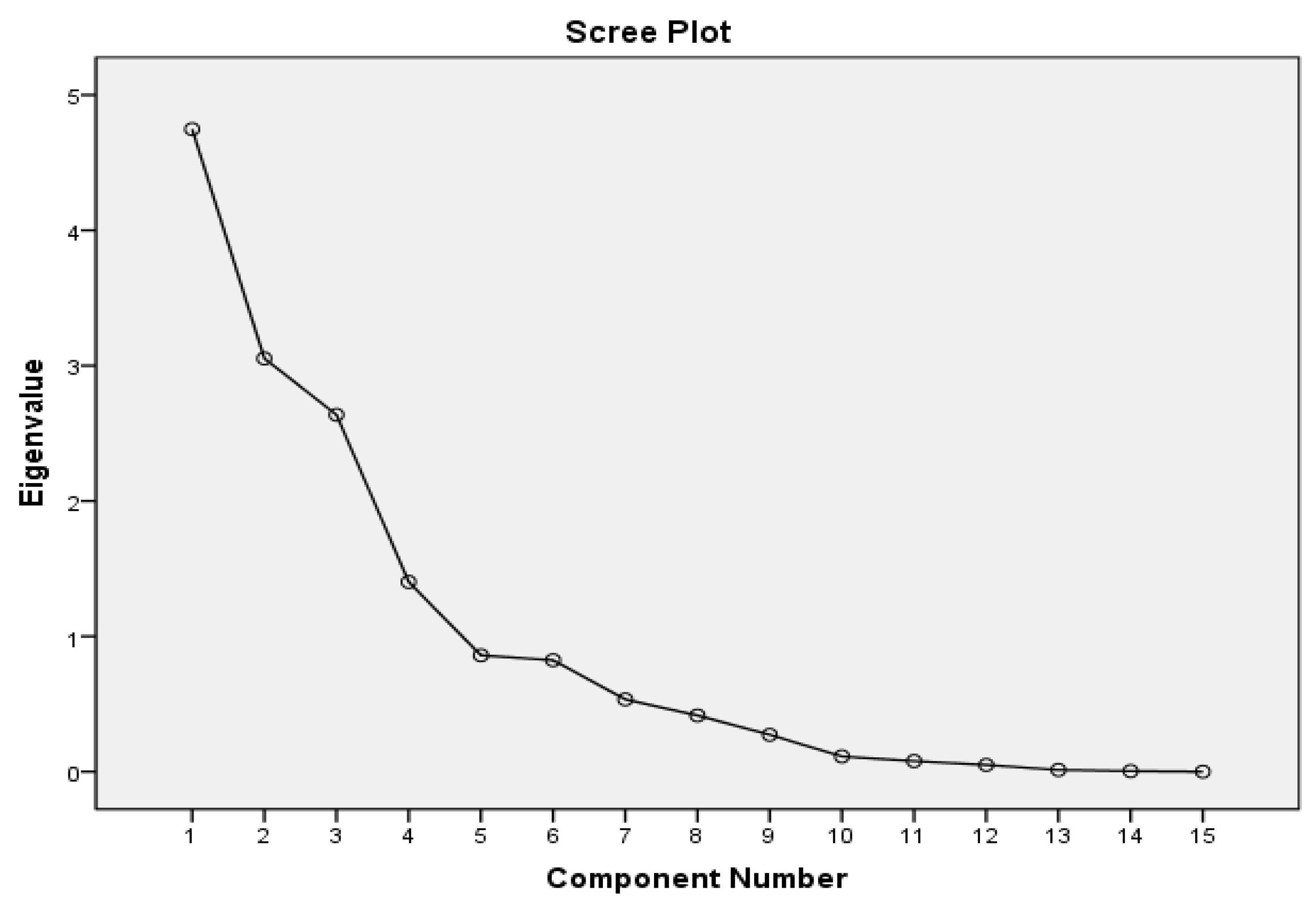
- Determine the number of factors to be extracted by observing the scree plot and the result of the total variance interpreted.
- Step 4.
- Implement the orthogonal rotation to the factor-loading matrix by the varimax method, and then output the result by the descending order of first factor loading. The rotated factor-loading matrix will be obtained at this step.
2.1.2. Phase 2—Calculate Entropy Weights
- Step 1.
- Determine the indicators that will be used to calculate the entropy weights of the net cost of the private sector, the public sector, or the users. Suppose that there are n indicators, and that each has m evaluation objects. A m × n matrix will be obtained at this step. aij (i = 1,2, …, m; j = 1,2, …n) is supposed to be an element of the matrix as the value of the i-th item in the j-th indicator.
- Step 2.
- Standardize the values of all of the items. a’ij is supposed to be the standardized value of an item. Use:for the indicator on which project has better performance when the value of aij is larger; or use:for the indicator on which project has the better performance when the value of aij is smaller.
- Step 3.
- Calculate the proportion yij of a’ij in the matrix.
- Step 4.
- Calculate the entropy value ej of every indicator.when , .
- Step 5.
- Calculate the difference coefficient dj of every indicator.
- Step 6.
- Calculate the entropy weight of every indicator.
2.1.3. Phase 3—Build the Optimization Model
- Step 1.
- Determine the decision variables of the optimization model based on the factor analysis results in Phase 1.
- Step 2.
- Determine the functions of the optimization model objectives and constraints by the PSC method.
- Step 3.
- Identify whether the optimization model has available solutions when it is required to satisfy the constraints that both the VFM and returns of the private sector are positive.
2.1.4. Phase 4—Get the Entropy-Weighted Results
- Step 1.
- Solve the optimization model by ‘gamultiobj’ solver on MATLAB 9.1.0.441655 (R2016b), and then get the Pareto solutions sets.
- Step 2.
- Calculate the entropy-weighted sum of each set in the Pareto front solution sets.
- Step 3.
- Find the minimum weighted sum, and the value set of its corresponding decision variables will be determined as the best quantitative decision of the project.
2.2. The Two Types of Optimization Models
There are usually two typical scenarios in the specific context of Chinese PPPs, so two types of optimization models need to be built.
For a newly-built PPP project, if there is no similar project built or under operation within the same city that could provide some guidance in project decision-making, i.e., there is no reference information of the project charge or concession period duration, etc., these pieces of information need to be treated as decision variables in the optimization model. However, the concrete discount rate to calculate the net present value (NPV) of the cost of the public sector should be determined as a parameter with a given value.
Else, if there are similar projects located within the same city, the project charge and concession period duration of the newly-built PPP project probably need to be consistent with the existing projects, i.e., these two parameters, charge and duration, should be treated as parameters with given values in the optimization model. In that scenario, the decision-makers of the public sector need to decide the discount rate within a reasonable range, i.e., the discount rate of the public sector cost could be treated as a decision variable.
In this paper, the optimization model of the first scenario is noted as ‘Model 1’, while that of the second scenario is noted as ‘Model 2’.
2.3. A URT PPP Project Case
Guizhou is a province located in southwest China that is well-known for its enriched tourism resources. The capital city is Guiyang city, where two URT lines are to be opened to the public. The case study in this paper is that of Line 2, which is planned to have eight stations: six underground and two on-the-ground. The total length of Line 2 will be 13 km: 9.83 km of underground sections, and 3.17 km of on-the-ground sections. The concession period duration is 29 years: four years of construction and 25 years of operation. The basic public investment benefit rate is 3–8%, the reported discount rate for the public sector is 6.22%, and the expected return rate for the private sector is 6.37%.
Table 1 listed the source data extracted from the project report [17], where Cci is the construction cost spent in the i-th year, yuan × 104; Coi is the operation cost spent in the i-th year, yuan × 104; Criski is the risk cost occurred in the i-th year, yuan × 104; Qi is the passenger turnover volume in the i-th year, km × 104; Di is the total planning operation kilometers of the i-th, km × 104, Ei is the project earning of the i-th year, yuan × 104; and Bi is the general public budget of Guiyang city of the i-th year, yuan × 108.
3. Results
3.1. The Factor Analysis
There were 15 different indicators used in the VFM qualitative evaluation of 19 URT PPP projects [17]: ‘Integration’ (I1), ‘Risk Allocation’ (I2), ‘Performance’ (I3), ‘Competitiveness’ (I4), ‘Government Competency’ (I5), ‘Bankability’ (I6), ‘Procurement Potential’ (I7), ‘Scale’ (I8), ‘Life span’ (I9), ‘Capital Diversity’ (I10), ‘Cost Accuracy’ (I11), ‘Legal Support’ (I12), ‘Income Potential’ (I13), ‘Exemplary’ (I14), and ‘Acceptance’ (15). In the current Chinese PPPs’ VFM evaluation system, the first six indicators are stipulated as basic ones that should be used in every PPP case, while the last 10 are specified as optional indicators that could be weighted as 0. In each PPP case, the sum of the weights is 1. Table A1 and Table A2 listed the original weights of the 15 indicators among 19 URT PPP projects, in which project 7 did not use the basic indicator ‘Bankability’.
Table 2 listed the correlation matrix of 15 indicators. Due to the existence of optional indicators, this matrix is not a positive definite, so that the BS test and KMO test could not proceed. Linear correlation could be seen between most indexes, which means these indicators could be used for factor analysis.
In Figure 1, the horizontal axis is the number of the factors that were supposed to be extracted, and the vertical axis is the eigenvalue of the factor. The eigenvalues of the first four factors are high, in which these factors have strong interpretation to 15 indicators. From the fifth factor to the last factor, their eigenvalues are low, i.e., these factors are weak in interpretation of all 15 indicators.
Table 3 is the component matrix of the four extracted factors. The loading of each indicator on the first factor is relatively higher than those of the other three factors. However, the meaning of these four factors is still obscure.
Table 4 displayed the rotated component matrix outputted in the first factor loading descending order. After orthogonal rotation of the original component matrix, the meanings of the four factors become clearer. As could be seen from Table 4, the loadings of ‘Procurement Potential’, ‘Capital Diversity’, ‘Government Competency’ and ‘Legal Support’ are high on the first factor, in which these indicators are the main components that are interpreted by the first factor. Similarly, the second factor provide interpretation mainly of ‘Performance’, ‘Competitiveness’, and ‘Scale’. The third factor mainly interpreted ‘Integration’ and ‘Life span’. The fourth factor mainly interpreted ‘Acceptance’.
From the above paragraph, it seems that the indicators that were mainly interpreted by the first factor on related to government commitments and guarantees; the second factor was associated with the output and performance of the private sector involvement; the third factor was directly related to concession period duration; and the fourth factor reflects the degree of the public service accepted by users who are supposed to be sensitive with price level. Thus, the decision variables could be determined as the benchmark benefit ratio of public investment (rg), which will be used as the discount rate of the public sector cost, the proportion of the public sector’s share in the project company (a), the unit payment to the private sector (b), and the public transport services charge to the users (p).
The degree of total variance interpreted by the extracted factors is shown in Table 5. There are two groups of datasets; each has three columns of data, in turns: the eigenvalue of the factor, the contribution rate of variance interpretation, and the accumulative contribution rate of variance interpretation. In the first group dataset, 78.923% of the total variance of the 15 indicators was interpreted by the four factors before rotation. The second group dataset is the ultimate factor solution after rotation. The accumulative contribution rate of variance interpreted after rotation is not changed. However, after rotation, the factor contributions to the 15 indicators are reallocated, and the meanings of the four factors are less obscure.
3.2. Two Nonlinear Multi-Objective Models
3.2.1. Model 1
Model 1 has three objectives: the minimum cost of the private sector, the public sector, or a single user, expressed as equations (7)–(9):
s.t.
and
a is the project share of the public sector, which is capped at 49% (according to current policy in China);
b is the unit payment for the private sector at every year, yuan/km;
p is the unit charge to users of the public transportation service provide by the PPP project, yuan/person/km;
n is the concession period duration, in years (in the 19 cases collected, the shortest duration is 10 years, and the longest one is 35 years.);
λg and λp are the coefficients that convert the present value into the unit time (e.g., every year) value;
CPRI is the net cost present value of the private sector, including the fund of equity share, the operating and maintenance cost, and risk expenditure (the payments from the public sector and users should be deducted);
CPUB is the net cost present value of the public sector, including the share funds, payment for the private sector, and risk expenditure;
CPSC is the Public Sector Comparator (PSC), which is the net cost present value of the public sector when implement the URT project in a traditional pattern other than the PPP pattern;
CVFM is the difference between CPSC and CPPP that reflects the savings of the public investment for using PPP instead of a traditional pattern;
Cpri is the unit cost undertaken by the private sector every year, yuan/person/km;
Cpub is the unit cost undertaken by the public sector every year, yuan/person/km;
Cuser is the unit cost of user, yuan/person/km, which is exactly the p;
Cc is the total investment of the project, which is also the sum of Cci in Table 1, 793293.91 yuan × 104;
rcap is the capital fund proportion of total investment, 30%;
Coy is the unit operating cost per year, 10.49, yuan/km/year, ;
rg is the minimum basic public investment benefit rate, 3%, which is also the discount rate for calculating the net cost present value of public sector;
rp is the minimum rate of return required by the private sector, 6.37%, which is also the discount rate for calculating the net cost present value of the private sector;
rt is the ratio of non-ticket revenue taken up to the total ticket revenue, 15%;
Eother is the ratio of the external commercial development revenue taken up to the total project investment, which is set at 20% to ensure that the optimization model does have available solutions.
3.2.2. Model 2
Model 2 has two objectives: the minimum cost of the private sector and the public sector, as expressed in equations (18) and (19). The cost of single user p is fixed in this scenario. Constraints are the same as with Model 1.
In Model 2, b is capped by 89.49. This value is calculated by:
which is stipulated by current PPP policy in China. Coi, Criski, Di, and Qi are listed in Table 1.
3.3. The Entropy Weights
The entropy weights of Cpri, Cpub, and Cuser in Model 1 are calculated on the variation degrees of Ei, Bi, and Qi in Table 1. The entropy weights of CPRI and CPPP in Model 2 are calculated by Ei, and Bi only.
Table 6 presents the weights of Cpri, Cpub, and Cuser of Model 1, where the weights of Cpri and Cuser are equal, and the weight of Cpub is the smallest.
Table 7 presents the weight of CPRI and CPPP of Model 2, where the weight of CPRI is larger than that of CPPP.
3.4. Pareto Front
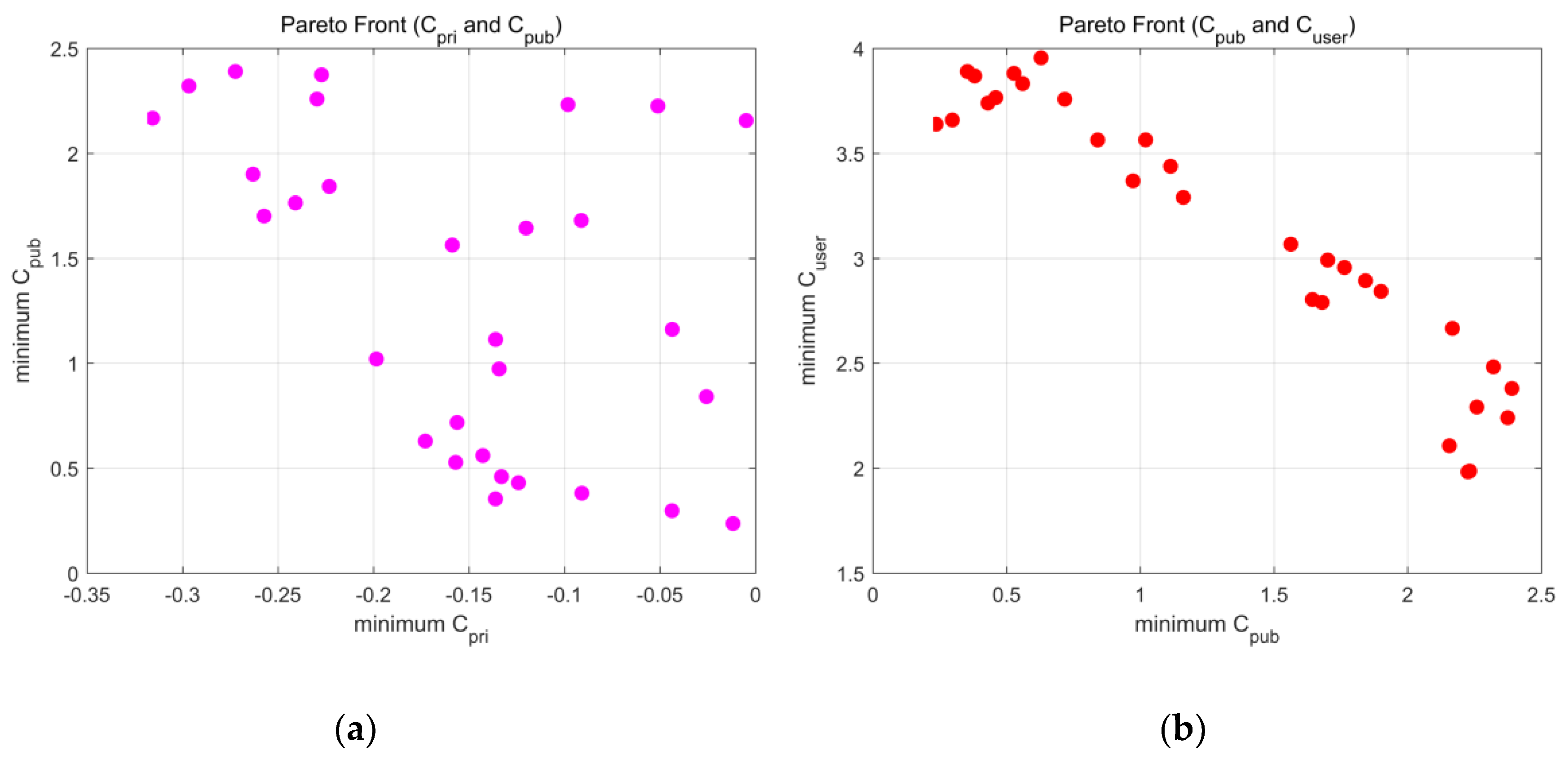
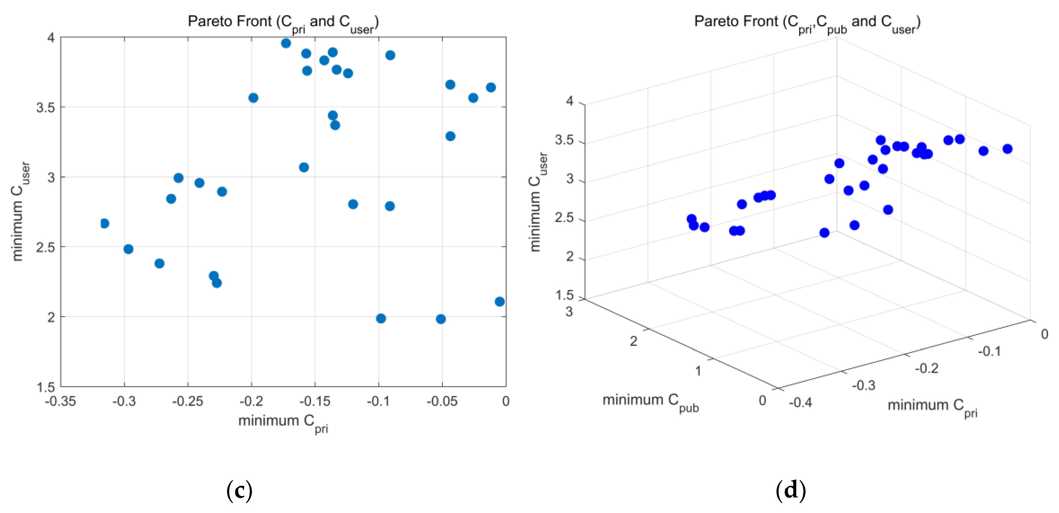
Figure 2 depicts the Pareto front of Model 1. Figure 2a–c presents the correlation between each pair of Cpri, Cpub, and Cuser, and Figure 2d presents the distribution of the Pareto solutions of the three objectives in a three-dimensional (3D) space. It seems that Cpub and Cuser are linear-correlated. However, it is not easy to determine the relation between Cpri and Cpub through the displayed complexion. Model 1 and Model 2 used the same configuration of the ‘gamultiobj’ solver to obtain optimized solutions. The maximum generation is set to 100,000, the initial population size is set to 1000, and the ratio of Pareto front to population size ratio is set to 0.3.
3.5. The Minimum Weighted Result
Table 8 is the minimum weighted sum and the value of the related decision variables and the value of the three objectives. Cpub is slightly more than Cuser, which means that the user paid less than the public sector to the project. The share ratio of the public sector was close to its upper limit, and the whole concession period duration was much shorter than the longest one of 19 cases (35 years).
As could be seen from Table 9, each decision variable is close to its own upper limit, and the net return obtained by the private sector through 25 years of operation exceeds the total investment of the project.
4. Discussion
From the collected 19 URT PPP project cases, it is understandable that to certain extent, the weight distribution among the 15 indicators in VFM qualitative evaluation reflected some of the quantifiable characteristics of the project that were valued by the experts who graded on the mark sheet. However, it may be difficult to directly obtain the correlation between the weight of the qualitative indicators and quantifiable characteristics. Factor analysis, as a common method of dimensionality reduction, could be used to explore such correlations by analyzing the data weights, and to find out the most important aspects and which qualitative evaluation indicators contributed to them substantially. Due to the application of the optional indicators in Chinese PPP practice, not all 15 indicators could be given non-zero weights, which then means that the correlation matrix is not positive definite, and the application of factor analysis tests are restricted. The unifying indicators in each evaluation may help in determining the quantitative decision variables with a more explanatory result factor analysis.
The entropy weight method is one kind of objective weighting that could avoid the bias caused by the expert preference that may occur in the subjective weighting methods. Under the same evaluation indicator, the greater the difference of the observed values, the smaller the entropy value of the corresponding indicator, and the greater the entropy weight. Initially, for Model 1, the author used the Pareto solutions directly as evaluation items under all three objectives—Cpri, Cpub, and Cuser—and found out that no matter how many times the experiment was conducted, the weights were equally distributed among the three evaluation indicators. The possible reason for that is the variance of observed values under each indicator produced by the solver equally. Thus, in order to reflect the difference degree of Cpri, Cpub, and Cuser, substituted indicators are needed.
This paper used Ei, Bi, and Qi as the entropy-weighting indicators for Model 1, because the operation cost in every year is fixed by Coy and Q. To be consistent with Model 1 in entropy-weighting, Model 2 selected Ei and Bi for calculating the weights of CPRI and CPUB. As seen from the results, in Model 1, the private sector and the users are equally weighted, and the public sector is slightly lower. In Model 2, the private sector has a slightly higher weight than the public sector. These results are basically consistent with the reality of Chinese PPPs practice, in which the public sector tent gives more benefits to the private sector and the users to enhance their willingness of participation, with non-negative VFM as the prerequisite of the project.
As seen in the Pareto front results of both Model 1 and Model 2, the private sector achieved profits based on the payment from the public sector and the users. In Model 1, b and p had the upper limit as positive infinity, while in Model 2, b had the upper limit and p was a constant parameter. However, b was much lower in Model 1 than in Model 2; since the users were burdened with a higher unit cost in Model 1, that unit price may be too expensive for the local citizen. In Model 2, in which the private sector yielded at a high level, the possible reason was that the decision variables a, b, and rg could not keep the private sector from over-profiting, reflecting that the current policies may not be reasonable.
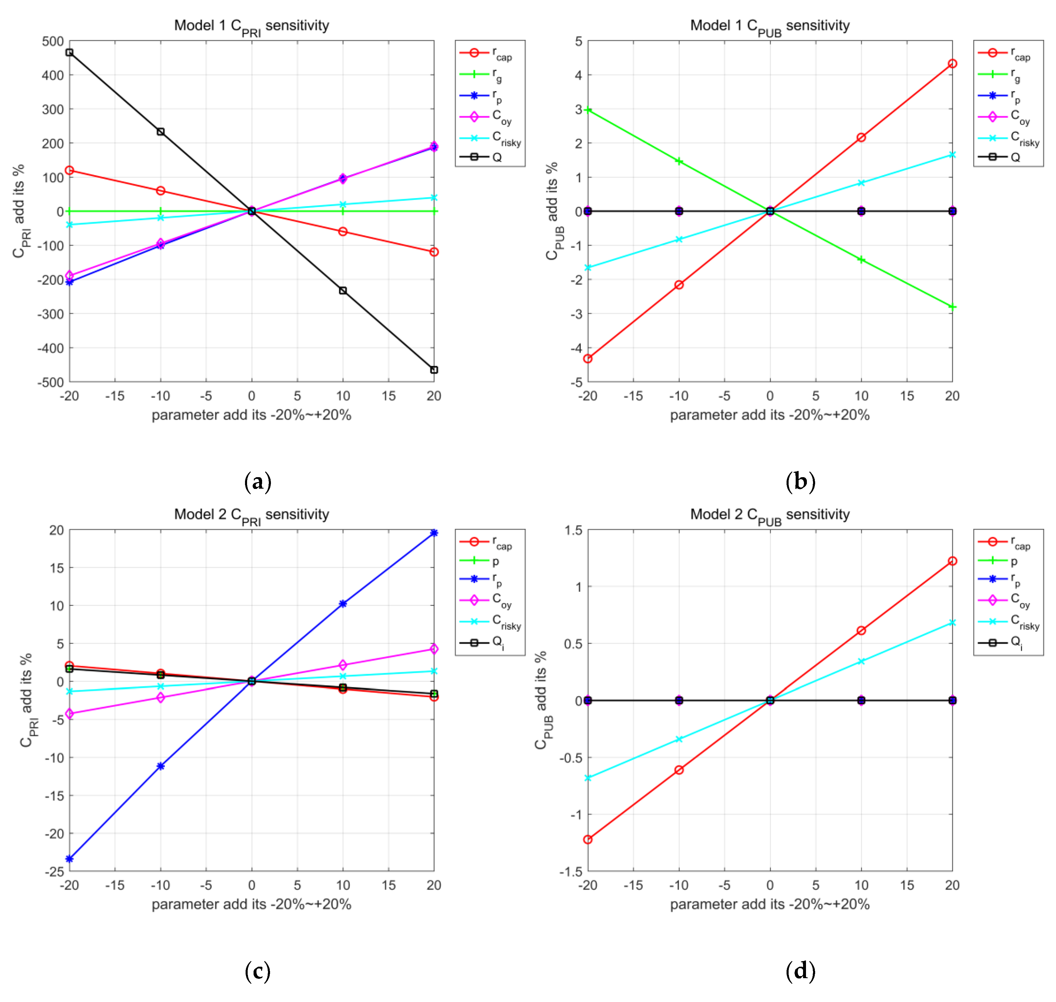
Figure 4 displays the variance (%) of CPRI and CPUB calculated by the decision picked out according to the minimum weighted sum in both models when some parameter added its own −20%, −10%, 0, +10%, +20%, respectively. Figure 4a shows that CPRI is very sensitive to most of the six parameters, rg and Criksy not included. Table 10 shows the actual values of CPRI when these parameters changed; the positive values are underlined, revealing that the private sector had a net loss, which failed to satisfy the prerequisites of a PPP project. Figure 4c presented that the CPRI value in Model 2 was insensitive to the parameters, except for rp. Figure 4b–d showed that CPUB was insensitive to the parameter changes in both models.
5. Conclusions
In this paper, factor analysis was carried out on the qualitative evaluation weights of the 19 URT PPP cases, and the results were used to determine the quantitative decision variables of the optimization models. Two types of nonlinear multi-objective models were established to solve the Pareto front solution sets, with constraints expressed as non-negative VFM values, and the return of the private sector upon the PSC method. The entropy-weights method was applied to evaluate the Pareto solutions, and the one with the minimum weighted sum was picked up. The calculated entropy weights showed consistency with the reality of Chinese PPPs practice. Finally, the sensitivity analysis of the present value of the public sector and private sector cost calculated by the determined decision variable value is obtained.
This paper provided a basic model under the scenario of static decision-making. The following two were not discussed throughout this article, but deserve further study:
One is the financing decision model of a cost-recovery URT PPP project based on add–value–capture (LVC) theory as the extension of the basic model in this paper. The other is the multi-stage dynamic and flexible decision-making problems over a whole life cycle of the URT PPP project, which can be divided into different stages of financing, bidding, construction, operation, maintaining, retrofitting, capital transferring, etc.
Author Contributions
F.L. contributed to the research design, data collection, implementation of model, and manuscript writing. J.L. and X.Y. acted as supervisory roles and contributed equally to problem analysis and the application of methodology.
Funding
This work is financially supported by National Natural Science Foundation (91746201).
Acknowledgments
This work was supported by China National Association of Engineering Consultants (CNAEC), which is gratefully acknowledged here. In addition, we thank Hannah Herchenbach, the editor of MDPI, for English editing of the final version of this manuscript.
Conflicts of Interest
The authors declare no conflicts of interest.
Appendix A
The VFM assessment reports of 19 URT PPP projects containing original manuscripts of grates and weights that listed in Table A1 and Table A2 are available online at http://www.cpppc.org:8086/pppcentral/map/toPPPList.do.

Table A1.
Part 1 of the original weights of 15 indicators from 19 URT PPP cases (Case 1 to 10).
| Case 1 | Case 2 | Case 3 | Case 4 | Case 5 | Case 6 | Case 7 | Case 8 | Case 9 | Case 10 | |
|---|---|---|---|---|---|---|---|---|---|---|
| Integration | 0.1 | 0.15 | 0.15 | 0.15 | 0.17 | 0.17 | 0.15 | 0.15 | 0.15 | 0.15 |
| Risk Allocation | 0.2 | 0.15 | 0.17 | 0.15 | 0.18 | 0.18 | 0.15 | 0.15 | 0.15 | 0.1 |
| Performance | 0.1 | 0.15 | 0.12 | 0.15 | 0.12 | 0.12 | 0.15 | 0.15 | 0.15 | 0.15 |
| Competitiveness | 0.2 | 0.1 | 0.13 | 0.15 | 0.08 | 0.08 | 0.15 | 0.15 | 0.15 | 0.15 |
| Government Competency | 0.1 | 0.1 | 0.13 | 0.05 | 0.13 | 0.13 | 0.05 | 0.05 | 0.1 | 0.1 |
| Bankability | 0.1 | 0.15 | 0.1 | 0.08 | 0.12 | 0.12 | 0 | 0.03 | 0.1 | 0.15 |
| Procurement Potential | 0 | 0 | 0 | 0.1 | 0 | 0 | 0.1 | 0.05 | 0 | 0 |
| Scale | 0 | 0 | 0.04 | 0 | 0.04 | 0.04 | 0.06 | 0.05 | 0.05 | 0.07 |
| Life span | 0 | 0 | 0 | 0 | 0.04 | 0.04 | 0 | 0.05 | 0 | 0 |
| Capital Diversity | 0 | 0 | 0 | 0.07 | 0.04 | 0.04 | 0.07 | 0.03 | 0 | 0 |
| Cost Accuracy | 0.1 | 0 | 0.05 | 0.05 | 0.08 | 0.08 | 0 | 0.03 | 0 | 0 |
| Legal Support | 0 | 0 | 0 | 0 | 0 | 0 | 0.07 | 0.03 | 0 | 0 |
| Income Potential | 0.1 | 0.08 | 0.04 | 0.05 | 0 | 0 | 0.05 | 0.05 | 0.05 | 0.07 |
| Exemplary | 0 | 0.06 | 0.07 | 0 | 0 | 0 | 0 | 0.03 | 0.1 | 0.06 |
| Acceptance | 0 | 0.06 | 0 | 0 | 0 | 0 | 0 | 0 | 0 | 0 |
Table A2.
Part 2 of the original weights of 15 indicators from 19 URT PPP cases (Case 11 to 19).
| Case 11 | Case 12 | Case 13 | Case 14 | Case 15 | Case 16 | Case 17 | Case 18 | Case 19 | |
|---|---|---|---|---|---|---|---|---|---|
| Integration | 0.15 | 0.13 | 0.15 | 0.15 | 0.15 | 0.15 | 0.15 | 0.15 | 0.15 |
| Risk Allocation | 0.15 | 0.15 | 0.2 | 0.2 | 0.15 | 0.15 | 0.15 | 0.15 | 0.15 |
| Performance | 0.15 | 0.12 | 0.1 | 0.1 | 0.15 | 0.15 | 0.15 | 0.15 | 0.15 |
| Competitiveness | 0.1 | 0.13 | 0.1 | 0.1 | 0.1 | 0.15 | 0.15 | 0.15 | 0.15 |
| Government Competency | 0.1 | 0.15 | 0.1 | 0.1 | 0.1 | 0.05 | 0.05 | 0.05 | 0.05 |
| Bankability | 0.15 | 0.12 | 0.15 | 0.15 | 0.15 | 0.15 | 0.1 | 0.04 | 0.1 |
| Procurement Potential | 0 | 0 | 0 | 0 | 0 | 0 | 0.03 | 0.1 | 0.03 |
| Scale | 0.06 | 0.06 | 0 | 0 | 0.04 | 0.05 | 0.03 | 0.06 | 0.03 |
| Life span | 0 | 0 | 0.05 | 0.05 | 0.03 | 0.05 | 0 | 0.04 | 0 |
| Capital Diversity | 0 | 0 | 0 | 0 | 0.04 | 0 | 0.04 | 0.06 | 0.04 |
| Cost Accuracy | 0 | 0.07 | 0.05 | 0.05 | 0.03 | 0.05 | 0.03 | 0 | 0.03 |
| Legal Support | 0 | 0 | 0 | 0 | 0 | 0 | 0.03 | 0 | 0.03 |
| Income Potential | 0.08 | 0.07 | 0.05 | 0.05 | 0.03 | 0.05 | 0.05 | 0.05 | 0.05 |
| Exemplary | 0.06 | 0 | 0.05 | 0.05 | 0.03 | 0 | 0.04 | 0 | 0.04 |
| Acceptance | 0 | 0 | 0 | 0 | 0 | 0 | 0 | 0 | 0 |
Table A3.
The full version of Pareto Front generated by Model and Model 2.
| Model 1 | Model 2 | ||||
|---|---|---|---|---|---|
| No. | Cpri | Cpub | Cuser | CPRI | CPUB |
| 1 | −0.01182 | 0.236268 | 3.638375 | −161,293 | 1,187,172 |
| 2 | −0.13615 | 0.353558 | 3.889556 | −1,261,708 | 2,305,979 |
| 3 | −0.05116 | 2.225221 | 1.982355 | −1,196,545 | 2,080,527 |
| 4 | −0.31566 | 2.167159 | 2.665843 | −987,204 | 1,898,145 |
| 5 | −0.04375 | 0.297243 | 3.658421 | −304,068 | 1,311,654 |
| 6 | −0.13424 | 0.972897 | 3.368459 | −1,260,641 | 2,159,870 |
| 7 | −0.0982 | 2.231788 | 1.98632 | −847,846 | 1,781,122 |
| 8 | −0.14278 | 0.560115 | 3.831897 | −821,201 | 1,764,332 |
| 9 | −0.13303 | 0.45965 | 3.765208 | −1,261,407 | 2,217,593 |
| 10 | −0.15699 | 0.527611 | 3.880541 | −1,224,720 | 2,116,505 |
| 11 | −0.12411 | 0.4304 | 3.73927 | −339,572 | 1,339,597 |
| 12 | −0.00492 | 2.1559 | 2.106714 | −281,836 | 1,294,707 |
| 13 | −0.29665 | 2.320473 | 2.482393 | −1,002,835 | 1,917,117 |
| 14 | −0.02571 | 0.840748 | 3.563561 | −321,014 | 1,336,837 |
| 15 | −0.09123 | 1.67997 | 2.789534 | −232,086 | 1,247,415 |
| 16 | −0.2296 | 2.258401 | 2.291057 | −728,035 | 1,680,591 |
| 17 | −0.13609 | 1.113198 | 3.438026 | −314,521 | 1,332,921 |
| 18 | −0.24086 | 1.763577 | 2.955981 | −356,058 | 1,366,419 |
| 19 | −0.19851 | 1.020047 | 3.563972 | −1,025,183 | 1,941,797 |
| 20 | −0.12015 | 1.643778 | 2.803375 | −486,996 | 1,474,725 |
| 21 | −0.26312 | 1.9003 | 2.842046 | −883,049 | 1,818,761 |
| 22 | −0.22314 | 1.842073 | 2.893234 | −1,131,454 | 2,036,124 |
| 23 | −0.22722 | 2.373951 | 2.240217 | −214,515 | 1,231,844 |
| 24 | −0.15876 | 1.562877 | 3.066917 | −1,039,812 | 1,948,281 |
| 25 | −0.15625 | 0.717709 | 3.757613 | −1,158,419 | 2,061,794 |
| 26 | −0.09092 | 0.380833 | 3.868423 | −1,123,306 | 2,016,009 |
| 27 | −0.27229 | 2.38963 | 2.379703 | −232,574 | 1,250,608 |
| 28 | −0.17288 | 0.628949 | 3.954517 | −840,417 | 1,771,252 |
| 29 | −0.2573 | 1.700806 | 2.991098 | −1,252,278 | 2,137,844 |
| 30 | −0.04364 | 1.161033 | 3.289835 | −250,612 | 1,264,479 |
References
- Cruz, C.O.; Marques, R.C. Theoretical considerations on quantitative PPP viability analysis. J. Manag. Eng. 2013, 30, 122–126. [Google Scholar] [CrossRef]
- Asian Development Bank (ADB); Inter-American Development Bank (IDB); World Bank Group; Public-Private Infrastructure Advisory Facility (PPIAF). Public-Private Partnerships: Reference Guide, Version 2.0; World Bank Group: Washington, DC, USA, 2014. [Google Scholar]
- Jiang, D.M.; Zhao, Z.; Management, S.O.; University, Q.T. Research on Investment Risk Management of Expressway PPP Project. Value Eng. 2017, 11, 35–38. [Google Scholar] [CrossRef]
- Jin, X.H. Neurofuzzy Decision Support System for Efficient Risk Allocation in Public-Private Partnership Infrastructure Projects. J. Comput. Civ. Eng. 2010, 24, 525–538. [Google Scholar] [CrossRef]
- Tang, Q. Research on the Risk of the PPP Project Based on the Cumulative Prospect Theory. Value Eng. 2017, 12, 69–71. [Google Scholar] [CrossRef]
- Yin, H.; Li, Y.; Zhao, D. Method of Decision Making of PPP Project Risk Allocation Scheme Based on Cloud Model. Scie. Technol. Manag. Res. 2016, 36, 201–206. [Google Scholar] [CrossRef]
- Song, B.; Fei, X.U. Partner-Selection in Public-Private Partnership Project Based on an Iterative Algorithm for the Multi-Objective Group Decision Problem. J. Syst. Manag. 2011, 20, 690–695. [Google Scholar]
- Xie, J.; Ng, S.T. Multiobjective Bayesian Network Model for Public-Private Partnership Decision Support. J. Constr. Eng. Manag. 2013, 139, 1069–1081. [Google Scholar] [CrossRef]
- Sharafi, A.; Iranmanesh, H.; Amalnick, M.S.; Abdollahzade, M. Financial management of Public Private Partnership projects using artificial intelligence and fuzzy model. Int. J. Energy Stat. 2016, 4, 1650007. [Google Scholar] [CrossRef]
- Xu, Y.; Sun, C.; Skibniewski, M.J.; Chan, A.P.C.; Yeung, J.F.Y.; Cheng, H. System Dynamics (SD)-based concession pricing model for PPP highway projects. Int. J. Proj. Manag. 2012, 30, 240–251. [Google Scholar] [CrossRef]
- Xue, Y.; Guan, H.; Corey, J.; Qin, H.; Han, Y.; Ma, J. Bilevel Programming Model of Private Capital Investment in Urban Public Transportation: Case Study of Jinan City. Math. Probl. Eng. 2015, 2015, 1–12. [Google Scholar] [CrossRef]
- Xue, Y.; Guan, H.; Corey, J.; Wei, H.; Yan, H. Quantifying a financially sustainable strategy of public transport: Private capital investment considering passenger value. Sustainability 2017, 9, 269. [Google Scholar] [CrossRef]
- Liu, J.; Yu, X.; Cheah, C.Y.J. Evaluation of restrictive competition in PPP projects using real option approach. Int. J. Proj. Manag. 2014, 32, 473–481. [Google Scholar] [CrossRef]
- Hu, Z.; Fan, X.F.; Dong, Q. Decision-making model of public-private partnerships projects’ paradigm choice—Based upon the SVM classified theory. J. Xi’an Univ. Archit. Technol. 2012, 4, 568–571. [Google Scholar] [CrossRef]
- Wang, Z.; Rangaiah, G.P. Application and Analysis of Methods for Selecting an Optimal Solution from the Pareto-Optimal Front obtained by Multi-Objective Optimization. Ind. Eng. Chem. Res. 2016, 56. [Google Scholar] [CrossRef]
- CPPPC China Public Private Partnerships Center—Project Database. Available online: http://www.cpppc.org:8086/pppcentral/map/toPPPList.do (accessed on 10 May 2018).
- Committee, G.M.T. Guiyang Rail Transit Line 2 Public Financing Feasiblity Report. Available online: http://www.cpppc.org:8083/efmisweb/ppp/projectLibrary/getProjInfoNational.do?projId=d4f66527c80b408f8a7729af7590fe1f (accessed on 10 May 2018).
Figure 1.
Scree plot chart of factor analysis.

Figure 2.
Pareto front solutions distribution chart of Model 1. (a) Cpri and Cpub; (b) Cpub and Cuser; (c) Cpri and Cuser; (d) Cpri, Cpub and Cuser.
Figure 2.
Pareto front solutions distribution chart of Model 1. (a) Cpri and Cpub; (b) Cpub and Cuser; (c) Cpri and Cuser; (d) Cpri, Cpub and Cuser.


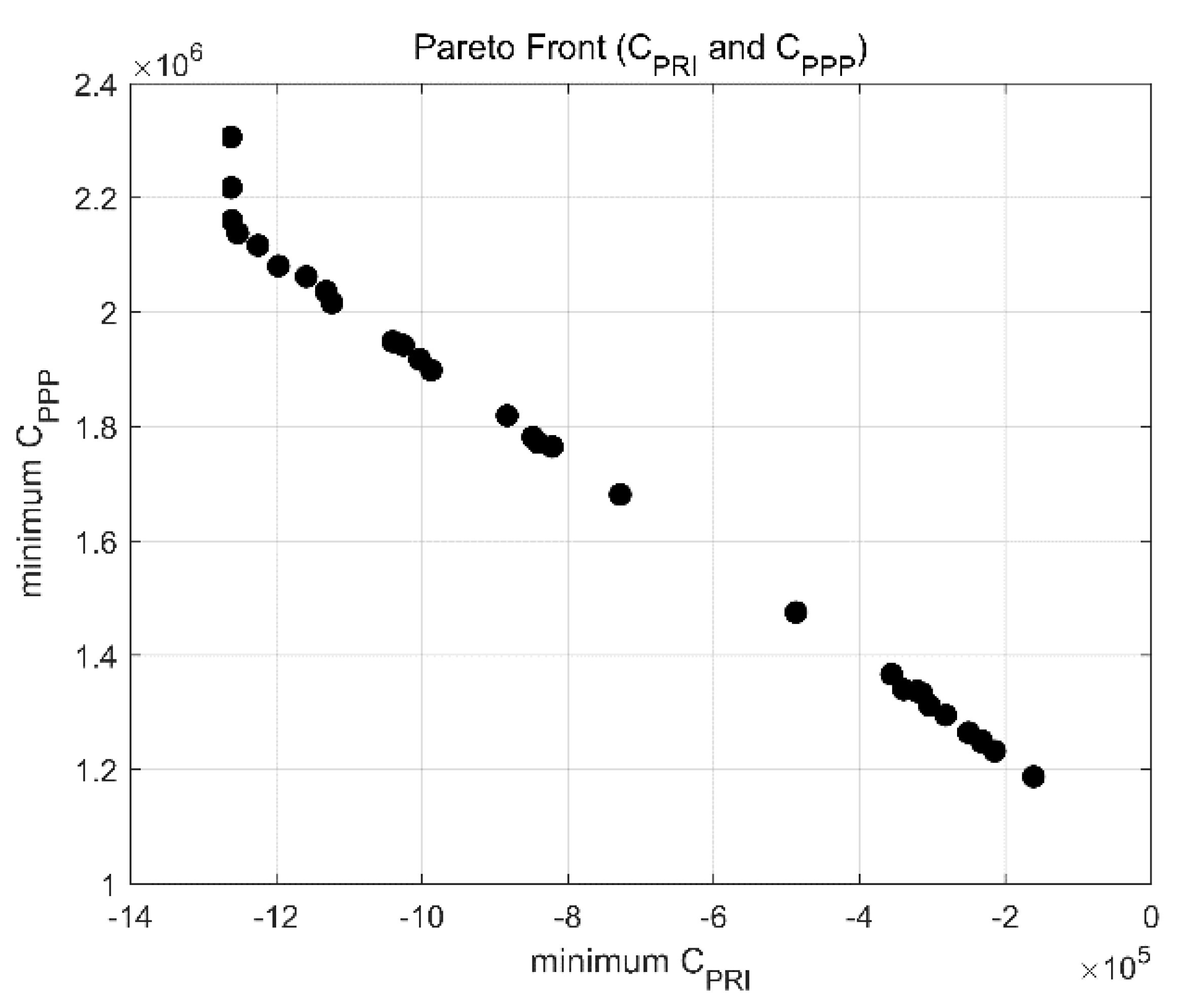
Figure 3.
Pareto front solutions distribution chart of Model 2.

Figure 4.
Sensitivity results of Model 1 and Model 2. (a) CPRI in Model 1, (b) CPUB in Model 1, (c) CPRI in Model 2, (d) CPUB in Model 2.
Figure 4.
Sensitivity results of Model 1 and Model 2. (a) CPRI in Model 1, (b) CPUB in Model 1, (c) CPRI in Model 2, (d) CPUB in Model 2.

Table 1.
Source data of Guiyang Urban Transit Railway (URT) Line 2 public–private partnerships (PPP) project.
Table 1.
Source data of Guiyang Urban Transit Railway (URT) Line 2 public–private partnerships (PPP) project.
| Year | i | Cci | Coi | Criski | Qi | Di | Ei | Bi |
|---|---|---|---|---|---|---|---|---|
| 2017 | 1 | 158,658.8 | 0 | 10,744.6 | 0 | 0 | 0 | 518.7 |
| 2018 | 2 | 237,988.2 | 0 | 16,116.89 | 0 | 0 | 0 | 534.26 |
| 2019 | 3 | 237,988.2 | 0 | 16,116.89 | 0 | 0 | 0 | 550.29 |
| 2020 | 4 | 158,658.8 | 0 | 10,744.6 | 0 | 0 | 0 | 566.79 |
| 2021 | 5 | 0 | 20,946.09 | 8629.92 | 9256.4 | 1933.07 | 3725.7 | 612.14 |
| 2022 | 6 | 0 | 20,946.09 | 8592.37 | 10,285.71 | 1933.07 | 4139.99 | 661.11 |
| 2023 | 7 | 0 | 20,946.09 | 8550.68 | 11,428.14 | 1933.07 | 4599.83 | 714 |
| 2024 | 8 | 0 | 20,624.54 | 8455.49 | 13,099.86 | 1933.07 | 5272.69 | 771.12 |
| 2025 | 9 | 0 | 20,624.54 | 8385.71 | 15,012.46 | 1933.07 | 6042.51 | 832.81 |
| 2026 | 10 | 0 | 20,624.54 | 8305.68 | 17,206.11 | 1933.07 | 6925.46 | 899.43 |
| 2027 | 11 | 0 | 20,624.54 | 8213.92 | 19,720.94 | 1933.07 | 7937.68 | 971.39 |
| 2028 | 12 | 0 | 20,624.54 | 8108.85 | 22,600.8 | 1933.07 | 9096.82 | 1049.1 |
| 2029 | 13 | 0 | 20,624.54 | 7988.34 | 25,904.06 | 1933.07 | 10,426.38 | 1133.03 |
| 2030 | 14 | 0 | 20,624.54 | 8224.58 | 19,428.94 | 1933.07 | 7820.15 | 1223.67 |
| 2031 | 15 | 0 | 22,433.06 | 8375.35 | 20,491.11 | 2188.19 | 8247.67 | 1260.38 |
| 2032 | 16 | 0 | 22,433.06 | 8334.6 | 21,608 | 2188.19 | 8697.22 | 1298.19 |
| 2033 | 17 | 0 | 22,433.06 | 8291.59 | 22,786.94 | 2188.19 | 9171.75 | 1337.13 |
| 2034 | 18 | 0 | 22,701.02 | 8277.53 | 24,031.6 | 2188.19 | 9672.72 | 1377.25 |
| 2035 | 19 | 0 | 22,701.02 | 8229.59 | 25,345.6 | 2188.19 | 10,201.6 | 1418.57 |
| 2036 | 20 | 0 | 22,701.02 | 8179.12 | 26,728.94 | 2188.19 | 10,758.4 | 1461.12 |
| 2037 | 21 | 0 | 22,701.02 | 8125.85 | 28,188.94 | 2188.19 | 11,346.05 | 1504.96 |
| 2038 | 22 | 0 | 22,701.02 | 8069.79 | 29,725.6 | 2188.19 | 11,964.55 | 1550.11 |
| 2039 | 23 | 0 | 22,701.02 | 8010.53 | 31,349.86 | 2188.19 | 12,618.31 | 1596.61 |
| 2040 | 24 | 0 | 22,701.02 | 8044.35 | 30,422.74 | 2188.19 | 12,245.16 | 1644.51 |
| 2041 | 25 | 0 | 22,701.02 | 8017.05 | 31,171 | 2188.19 | 12,546.33 | 1693.84 |
| 2042 | 26 | 0 | 22,701.02 | 7989.09 | 31,937.51 | 2188.19 | 12,854.84 | 1744.66 |
| 2043 | 27 | 0 | 22,701.02 | 7960.46 | 32,722.26 | 2188.19 | 13,170.71 | 1797 |
| 2044 | 28 | 0 | 22,701.02 | 7931.16 | 33,525.26 | 2188.19 | 13,493.91 | 1850.91 |
| 2045 | 29 | 0 | 22,701.02 | 7901.06 | 34,350.14 | 2188.19 | 13,825.94 | 1906.43 |
Table 2.
Correlation matrix of 15 indicators.
| I1 | I2 | I3 | I4 | I5 | I6 | I7 | I8 | I9 | I10 | I11 | I12 | I13 | I14 | I15 | |
|---|---|---|---|---|---|---|---|---|---|---|---|---|---|---|---|
| I1 | 1.000 | −0.164 | 0.286 | −0.678 | −0.015 | 0.057 | 0.067 | 0.236 | 0.370 | 0.336 | −0.258 | 0.053 | −0.783 | 0.117 | 0.027 |
| I2 | −0.164 | 1.000 | −0.841 | −0.255 | 0.300 | 0.112 | −0.238 | −0.637 | 0.414 | −0.146 | 0.667 | −0.187 | −0.179 | −0.162 | −0.095 |
| I3 | 0.286 | −0.841 | 1.000 | 0.219 | −0.591 | −0.279 | 0.429 | 0.484 | −0.296 | 0.388 | −0.739 | 0.337 | 0.055 | 0.114 | 0.171 |
| I4 | −0.678 | −0.255 | 0.219 | 1.000 | −0.522 | −0.489 | 0.383 | 0.072 | −0.395 | 0.066 | −0.061 | 0.302 | 0.558 | −0.119 | −0.230 |
| I5 | −0.015 | 0.300 | −0.591 | −0.522 | 1.000 | 0.514 | −0.701 | 0.008 | −0.053 | −0.522 | 0.419 | −0.552 | −0.142 | 0.166 | 0.080 |
| I6 | 0.057 | 0.112 | −0.279 | −0.489 | 0.514 | 1.000 | −0.821 | −0.256 | 0.096 | −0.662 | 0.180 | −0.694 | 0.063 | 0.336 | 0.224 |
| I7 | 0.067 | −0.238 | 0.429 | 0.383 | −0.701 | −0.821 | 1.000 | 0.099 | −0.069 | 0.817 | −0.318 | 0.543 | −0.026 | −0.420 | −0.139 |
| I8 | 0.236 | −0.637 | 0.484 | 0.072 | 0.008 | −0.256 | 0.099 | 1.000 | −0.073 | 0.096 | −0.393 | 0.217 | −0.143 | −0.031 | −0.356 |
| I9 | 0.370 | 0.414 | −0.296 | −0.395 | −0.053 | 0.096 | −0.069 | −0.073 | 1.000 | 0.035 | 0.264 | −0.190 | −0.502 | −0.274 | −0.197 |
| I10 | 0.336 | −0.146 | 0.388 | 0.066 | −0.522 | −0.662 | 0.817 | 0.096 | 0.035 | 1.000 | −0.096 | 0.517 | −0.456 | −0.545 | −0.207 |
| I11 | −0.258 | 0.667 | −0.739 | −0.061 | 0.419 | 0.180 | −0.318 | −0.393 | 0.264 | −0.096 | 1.000 | −0.301 | −0.249 | −0.511 | −0.282 |
| I12 | 0.053 | −0.187 | 0.337 | 0.302 | −0.552 | −0.694 | 0.543 | 0.217 | −0.190 | 0.517 | −0.301 | 1.000 | −0.021 | −0.160 | −0.109 |
| I13 | −0.783 | −0.179 | 0.055 | 0.558 | −0.142 | 0.063 | −0.026 | −0.143 | −0.502 | −0.456 | −0.249 | −0.021 | 1.000 | 0.212 | 0.289 |
| I14 | 0.117 | −0.162 | 0.114 | −0.119 | 0.166 | 0.336 | −0.420 | −0.031 | −0.274 | −0.545 | −0.511 | −0.160 | 0.212 | 1.000 | 0.226 |
| I15 | 0.027 | −0.095 | 0.171 | −0.230 | 0.080 | 0.224 | −0.139 | −0.356 | −0.197 | −0.207 | −0.282 | −0.109 | 0.289 | 0.226 | 1.000 |
Table 3.
Component matrix.
| Component | ||||
|---|---|---|---|---|
| 1 | 2 | 3 | 4 | |
| Procurement Potential | 0.841 | 0.292 | −0.203 | 0.207 |
| Government Competency | −0.777 | −0.040 | 0.159 | −0.294 |
| Bankability | −0.773 | −0.289 | 0.308 | 0.018 |
| Performance | 0.762 | −0.315 | 0.434 | 0.033 |
| Legal Support | 0.712 | 0.136 | −0.126 | 0.087 |
| Capital Diversity | 0.700 | 0.588 | 0.015 | 0.165 |
| Risk Allocation | −0.604 | 0.485 | −0.423 | 0.265 |
| Cost Accuracy | −0.572 | 0.508 | −0.492 | −0.173 |
| Income Potential | 0.051 | −0.789 | −0.511 | 0.083 |
| Life span | −0.258 | 0.647 | 0.177 | 0.062 |
| Exemplary | −0.205 | −0.628 | 0.397 | 0.105 |
| Integration | 0.097 | 0.434 | 0.853 | 0.135 |
| Competitiveness | 0.500 | −0.338 | −0.679 | −0.218 |
| Scale | 0.426 | −0.078 | 0.417 | −0.732 |
| Acceptance | −0.126 | −0.423 | 0.190 | 0.716 |
Extraction method: principal component analysis.
Table 4.
The rotated composition matrix.
| Component | ||||
|---|---|---|---|---|
| 1 | 2 | 3 | 4 | |
| Procurement Potential | 0.928 | 0.120 | −0.026 | −0.017 |
| Capital Diversity | 0.858 | 0.021 | 0.340 | −0.110 |
| Bankability | −0.841 | −0.052 | 0.127 | 0.226 |
| Government Competency | −0.785 | −0.244 | 0.142 | −0.149 |
| Legal Support | 0.706 | 0.205 | −0.074 | −0.062 |
| Exemplary | −0.505 | 0.480 | −0.088 | 0.336 |
| Risk Allocation | −0.122 | −0.890 | 0.120 | 0.164 |
| Cost Accuracy | −0.182 | −0.868 | 0.022 | −0.266 |
| Performance | 0.396 | 0.842 | 0.022 | 0.048 |
| Integration | 0.053 | 0.319 | 0.916 | 0.044 |
| Income Potential | −0.110 | 0.141 | −0.888 | 0.268 |
| Competitiveness | 0.412 | 0.060 | −0.806 | −0.220 |
| Lifespan | 0.012 | −0.398 | 0.596 | −0.084 |
| Acceptance | −0.139 | 0.190 | −0.029 | 0.829 |
| Scale | 0.015 | 0.630 | 0.102 | −0.700 |
Extraction method: principal component analysis. Rotation method: Varimax with Kaiser normalization. Rotation converged in five iterations.
Table 5.
The total variance interpreted by four extracted factors.
| Extraction Sums of Squared Loadings | Rotation Sums of Squared Loadings | ||||
|---|---|---|---|---|---|
| Total | % of Variance | Cumulative % | Total | % of Variance | Cumulative % |
| 4.747 | 31.647 | 31.647 | 4.082 | 27.211 | 27.211 |
| 3.053 | 20.354 | 52.001 | 3.323 | 22.150 | 49.361 |
| 2.636 | 17.577 | 69.578 | 2.825 | 18.834 | 68.195 |
| 1.402 | 9.345 | 78.923 | 1.609 | 10.728 | 78.923 |
Table 6.
The entropy weights of Cpri, Cpub, and Cuser in optimization Model 1.
| of | Cpri | Cpub | Cuser |
|---|---|---|---|
| entropy value | 0.909389 | 0.934844 | 0.909388 |
| entropy weight | 0.367772 | 0.264454 | 0.367774 |
Table 7.
The entropy weights of CPRI and CPUB in optimization Model 2.
| of | CPRI | CPUB |
|---|---|---|
| entropy value | 0.909389 | 0.934844 |
| entropy weight | 0.58171 | 0.41829 |
Table 8.
The minimum entropy-weighted sum of Pareto solutions of Model 1.
| a | b | p | n | Cpri | Cpub | Cuser | Weighted Sum |
|---|---|---|---|---|---|---|---|
| 0.487381 | 17.64895 | 1.98632 | 12.38446 | -0.0982 | 2.231788 | 1.98632 | 1.284605 |
Table 9.
The minimum entropy-weighted sum of Pareto solutions of Model 2.
| a | b | rg | CPRI | CPUB | Weighted Sum |
|---|---|---|---|---|---|
| 0.487917 | 89.15039 | 0.079737 | −1,252,278 | 2,137,844 | 165,775.7 |
Table 10.
The minimum entropy-weighted sum of the Pareto solutions of the optimization of Model 1.
| −20% | −10% | 0 | 10% | 20% | |
|---|---|---|---|---|---|
| when rcap changed | 3804.055 | −7795.05 | −19,394.1 | −30,993.3 | −42,592.4 |
| when rg changed | −19,394.1 | −19,394.1 | −19,394.1 | −19,394.1 | −19,394.1 |
| when rp changed | −59,664.9 | −38,980.1 | −19394.1 | −835.989 | 16,760.19 |
| when Coy changed | −56,123.2 | −37,758.7 | −19,394.1 | −1029.62 | 17,334.92 |
| when Crisky changed | −27,075.6 | −23,234.9 | −19,394.1 | −15,553.4 | −11,712.7 |
| when Qi changed | 70,829.07 | 25,717.46 | −19,394.1 | −64,505.8 | −109,617 |
© 2018 by the authors. Licensee MDPI, Basel, Switzerland. This article is an open access article distributed under the terms and conditions of the Creative Commons Attribution (CC BY) license (http://creativecommons.org/licenses/by/4.0/).
Share and Cite
MDPI and ACS Style
Liu, F.; Liu, J.; Yan, X. Quantifying the Decision-Making of PPPs in China by the Entropy-Weighted Pareto Front: A URT Case from Guizhou. Sustainability 2018, 10, 1753. https://doi.org/10.3390/su10061753
AMA Style
Liu F, Liu J, Yan X. Quantifying the Decision-Making of PPPs in China by the Entropy-Weighted Pareto Front: A URT Case from Guizhou. Sustainability. 2018; 10(6):1753. https://doi.org/10.3390/su10061753
Chicago/Turabian StyleLiu, Feiran, Jun Liu, and Xuedong Yan. 2018. "Quantifying the Decision-Making of PPPs in China by the Entropy-Weighted Pareto Front: A URT Case from Guizhou" Sustainability 10, no. 6: 1753. https://doi.org/10.3390/su10061753
Note that from the first issue of 2016, this journal uses article numbers instead of page numbers. See further details here.