A Research on the Debt Sustainability of China’s Major City Governments in Post-Land Finance Era


1
Department of Accounting, School of Business Administration, Northeastern University, Shenyang 110167, China
2
Department of Management, School of Economics and Management, University of Bologna, 47121 Forlì Campus, Italy
*
Author to whom correspondence should be addressed.
Sustainability 2018, 10(5), 1606; https://doi.org/10.3390/su10051606
Submission received: 13 April 2018
/
Revised: 11 May 2018
/
Accepted: 15 May 2018
/
Published: 17 May 2018
(This article belongs to the Section Economic and Business Aspects of Sustainability)
Abstract
:Land finance, i.e., a city government’s revenue, depends deeply on the revenue from transferring multiannual land use rights and is a phenomenon unique to China. However, due to increasingly tense land supply, increasingly prominent social conflicts, and the slowdown of urbanization in China, the country is entering what we may label the “post-land finance” era. Therefore, revenue from land finance is decreasing, which threatens the sustainability of Chinese city governments’ debt, especially in major cities. This paper tests the long-term sustainability of major Chinese city governments’ debt. Different from intuition, the empirical results show that the debt of these major city governments is still sustainable at the macro level. This paper also constructs a quadratic function model to predict the critical value of the local government debt. Our results suggest that despite the fact that debt is still sustainable, critical value may be reached quickly, as debt is growing rapidly. There is thus a need for local fiscal reform that divides financial power and authority between the local governments and the central government more reasonable and clearly, improves the current assessment mechanism of local governments’ officials, and speeds up the legislative work on property taxes.
1. Introduction
A significant portion of the gross domestic product of most industrialized countries is produced in their metropolitan regions: cities, towns, and other local government (LG) entities. By 2025, 600 cities in the world are projected to generate more than 60% of global GDP [1]. In Europe, 67% of GDP is generated in these areas [2], while in the U.S., Canada, and Australia, the figures are 85%, 72%, and 80%, respectively [3,4,5]. Similar percentages exist for some of the so-called non-industrialized countries, especially those in Latin America and Asia-Pacific, where the percentages range from 60% to 80% [6,7]. Moreover, even if the portion of GDP produced in a region’s metropolitan areas is relatively low, the public expenditures that take place in these areas can be a significant portion of total public expenditures. In China, expenditures in LGs constitute more than 80% of total public expenditures, one of the highest percentages in the world [8]. It thus seems clear that improved financial management of LGs is a key ingredient in the future growth, prosperity, and sustainability of both industrialized and non-industrialized countries across the globe, especially in an era where crises may require them to be ready for resilience [9].
Land finance is a term with very Chinese characteristics in LGs’ fiscal setting, and it is a phenomenon that attracts much public attention in recent years. Land finance means that LGs’ fiscal revenue is very dependent on the revenue from transferring multiannual land use rights. In China, with respect to the land ownership, there are two possibilities: land owned by the central state, and land collectively owned by peasants. No private ownership of land is allowed in China. LGs buy the land collectively owned by peasants, usually at a low price with the aim to urbanize. This way the ownership of these lands is converted from collective ownership to public ownership, and this represents the land finance expenditure. Then, LGs transfer the land to the real estate developers at higher prices through competitive bidding: the revenue of land finance comes from this process. It should be emphasized that the transfer from LGs to the developers refers to the land use rights, which is usually 70 years, not the ownership. Real estate developers transfer the land use rights and the apartments built to buyers. Many of the buyers are also peasants themselves. The urbanization rate in China was ca. 55% in 2014; this means that about half of Chinese are still peasants [10], and, according to the understanding of the central government of China, the urbanization will increase further. After the 70 years expire, from the angle of law principle, the land and buildings should return to the State. However, the reality now is that buyers do not pay for the use of the land again, or pay only a very small fee [11]. Jiang Daming, the Minister of China’s Ministry of land and resources, said to the journalists at a high-level meeting in China on 3 January 2018 that the owners do not need to pay many additional fees after the 70 years expire, and even the owners do not have to apply to the relevant departments for a renewal of the land use right; the land use right will be renewed automatically [12]. Therefore, in fact, transferring land use rights by LGs is very similar to land selling, and LGs can only get a lump-sum that they receive just once. For this reason, the words land selling will also be sometimes used below. Land finance can thus be viewed from two perspectives: From the perspective of the central government, it is a policy to increase the urbanization of China, and from the perspective of LGs, it is a source of capital local revenue.
After the tax-sharing reform of 1994, the revenue from land finance has become the main source of finance for LGs in China [13]. Table 1 clearly shows that this kind of revenue accounts for about half of the total revenue of LGs in recent years, but at the same time this proportion is showing a declining trend.
1.1. Local and City Governments in China
China represents the country with the highest percentage of LGs expenditure out of total public expenditures in the world, corresponding to about 20% of national GDP [8]. There are five levels of LG: the provincial level (province, autonomous region, municipality, and special administrative region) and, in order of importance, the city, county, township, and village levels. The central government is only responsible for national defense, diplomatic, and other related expenditures, while almost all the other functions, and thus related expenses, are borne by LGs [14]. The four municipalities (Beijing, Shanghai, Tianjin, and Chongqing) are on the same political administrative level as the provinces, even though they are large cities. The implementation of land finance is at both municipal and city government level. There is a city classification based on their importance that divides Chinese cities into five levels [15]. The first and second tier cities plus the four big municipalities represent the 41 major cities, which account for about a half of national GDP in 2016. The 41 major Chinese cities are listed in Table 2.
1.2. How Did the Land Finance of China Come Up?
One reason relates to the evolution of China’s public financial system. Before 1994, the public finance system that China implemented was called Fiscal Responsibility System (FRS). According to FRS, the central government would consider the revenue of each LG in the previous years, then gave each LG a basement to handover part of the revenue to the central government. After handing over part of the revenue to the central government, LGs could arrange the remaining revenue freely. However, this public finance management of FRS did not consider the differences between different taxes. Hussain & Stern (1992) [16] pointed out that FRS had a series of problems, for example, under this kind of system, the vitality of enterprises was bound, local protectionism increased, low level repeated construction increased, and the financial relationship between the central government and LGs under FRS was not stable and unclear. Park et al. (1996) [17] believed that the FRS led to the bargain on the revenue between the central government and LGs, and brought about the problem of soft budget constraints; the formal fiscal transfer between different governments could not be formed.
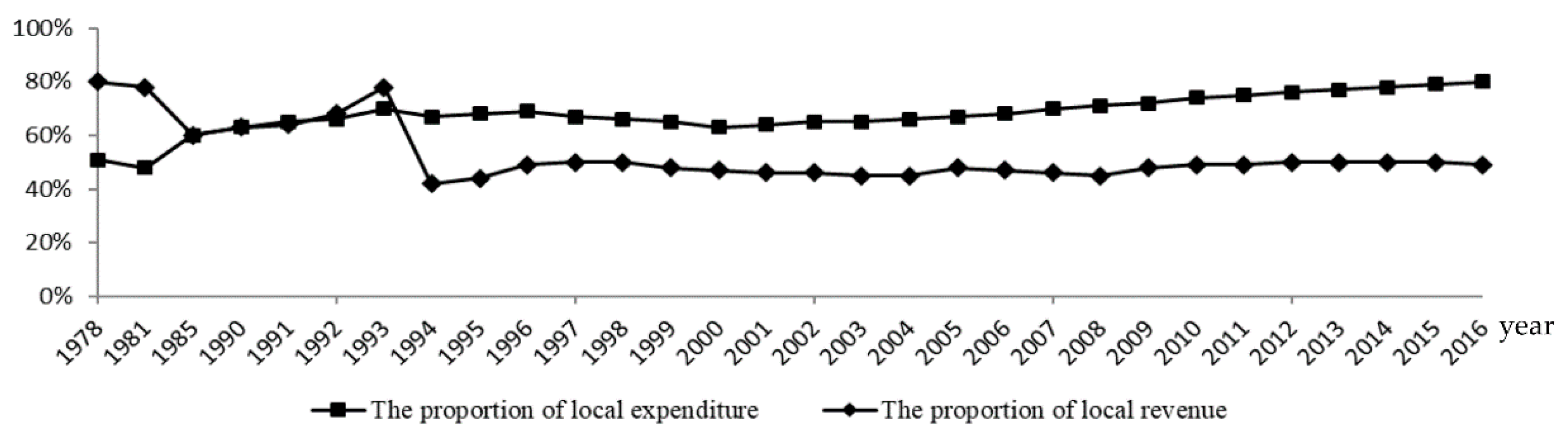
These authors and other scholars, like Liou (2011) [18], believed that another kind of public finance system, the Tax Sharing System (TSS), widely implemented in other market economies, would be helpful for overcoming these shortcomings. In 1994, the State Council issued a decision on the implementation of the TSS for public fiscal management. The TSS consists of three main aspects: the division of central and local taxes, the division of power and expenditure between central government and LGs, and the fiscal transfer policy. So, the budget law that China implements now is the version that was revised in 2014. The reasons why the central government implements the TSS are, on the one hand, to overcome the shortcomings of FRS, and, on the other hand, to deepen the reform of the socialist market economy of China and improve the revenue of the central government [19,20]. However, the TSS also leads to the problem of land finance in China. After the implementation of the TSS, the expenditure of LGs has increased, but LGs’ revenue has not raised correspondingly. We can see from Figure 1 that from 1994, the local expenditure has increased gradually: in 2016, it accounts for about 80%, but the proportion of local revenue is just about 50%.
Table 3 portrays city governments’ main revenue and expenditure. General public expenditure refers to those daily expenditures to ensure the normal operation of cities, similar to current expenditures, and non-general public expenditure refers to those non-daily expenditures, or capital expenditures plus expenditures for debt service. Social insurance funds (pensions) are not included here, because they constitute a separate budget and financial management system. Revenues are grouped into two types: revenues from taxes and non-tax revenues. Among the latter, revenues from land finance is included. This type of revenue is used to cover “expenditure on urban infrastructure construction (1.14)”; “land finance related expenditure (2.1)” (for example, the payments for the transferring land, expenses for resettlement of peasants, and subsidies for lost crops grown on transferring land); “debt repayment expenditures (2.2)”, many of which are loans from banks also using for infrastructure construction; and related “interest expenditure (2.3)”. Details about land finance expenditures are listed in the methods section (Table 4). It should be noted that the structure of financial reports is different in different cities, and this structure represents the “minimum common denominator” structure [21].
According to Sun & Zhou (2014) [22], in recent years the central government has received more than half of the total revenue, but the proportion of its total expenditure is only about 20%, causing a surplus at the central government level (used mainly to subsidize the western poor areas, or to purchase other countries’ treasury bonds) and a deficit at the level of LGs. This requires local governments to find new sources of income, and after the central government liberalized some relevant restrictions of “selling land”, the phenomenon of land finance appeared.
Another reason relates to the assessment mechanism of LGs’ officials. In China, the promotion of LGs’ officials is largely based on the growth of their local GDP [23], and the income from land finance can be invested in real estate and other infrastructure construction. It is widely accepted that the investment of real estate and other infrastructure construction can improve the local GDP as quickly as possible [24,25]. Then, LGs’ officials will have a greater chance of promotion.
Therefore, the imbalance of revenue and expenditure between the central and local governments under the TSS, and the assessment mechanism of LGs’ officials based on GDP growth, cause the phenomenon of land finance in today’s China.
1.3. China is Entering a “Post-Land Finance” Era
From Table 1, we can also notice that both the selling area and the revenue related to land finance show a downward trend in recent years, and although the revenue may increase in a certain year (as the price of land increases), the growth rate of it has slowed down. In addition, the proportion of land finance revenue to total local fiscal revenue is also becoming smaller. These are the intuitive manifestations of the land finance decline. The underlying reasons for the unsustainability of China’s land finance can be seen from the following aspects.
First, the supply of land is limited. From a macroscopic point of view, for the development of the urbanization of the country, China should supply urban development land every year and transform farmland or other kinds of agricultural land into urban construction land, but this would threaten the food security of the Chinese people [26]. According to Huang Qifan [27], the vice Chairman of the Financial and Economic Committee of the National People’s Congress of China, during the past 30 years since the Reform and Opening-up, China’s arable land has been reduced by more than 300 million mu (1 mu is equal to 667 square meters). In 1980, the cultivated land area of the country was 2 billion 300 million mu; by 2017, the cultivated land area had dropped to 2 billion mu, which is not enough to solve the Chinese eating problem, and therefore China has to import feed or grain from abroad every year [28]. For example, in 2014, the self-sufficiency rate of China’s agricultural products was only about 70% [29]. So, the red line of China’s cultivated land must be kept, which is related to the national security of China [30]. In a word, the food security determines that China’s land supply is limited.
Second, the finiteness of urban expansion determines the unsustainability of land finance. As mentioned above, in 2014, the level of urbanization in China was about 55%. According to Shi et al. (2016) [31], China is now in the accelerating stage of urbanization, and when the proportion of urban population accounts for about seventy percent of the total population, the growth trend of urban population will be slowed or even stagnated; then, the demand for urban land will also be stable. Therefore, when the level of urbanization tends to be stable, the current land finance model based on the expansion of urban land in China will also be difficult to continue.
Third, to a certain extent, land finance violates the social equity principle. The unfairness of land finance is mainly reflected in two respects. One the one hand, the income distribution between LGs and landless farmers is unfair [32]. LGs take advantage of the defects of the existing land system to collect farmers’ land at low prices and sell it at high prices; in the process of the land sale, farmers have no substantial pricing power for the price of land sold [33], and the power to operate the land is actually monopolized by LGs. Most of the income of land value added is occupied by LGs and other real estate developers at all levels, but farmers who have lost their land get only a few one-time compensation payments in the process of land expropriation. So, farmers cannot share the benefits of the growth of land value. On the other hand, intergenerational injustice exists among those LGs. As a matter of fact, current LGs tend to overdraft the land for sale, so less and less land can be sold by future LGs, and then the expansion capacity of local cities will be restricted. Furthermore, an important function of land finance is to finance urban infrastructure construction, but a government has only 5 years in office, and the governments’ land pledge loan is often left to future governments to pay back. This poses a great risk to future governments’ finances, and, also, it is extremely unfair to them. Last, besides the above aspects, the existing land financial system in China also causes low efficiency of land use, because many apartments cannot be sold out, or even if they are sold, the owners speculate and do not live there, so many of these areas become “ghost towns” [34]. The construction of these buildings has taken a lot of manpower, financial resources, and material resources, but no one has lived in them, so the number of people on this kind of land per square kilometer can be zero. This has caused the idleness and waste of resources, because the previous arable land can even be used to grow crops. In conclusion, no matter from the perspective of demand and supply of the land, or from the perspective of fairness and efficiency, the current land finance system that Chinese LGs are now implementing is unstable and unsustainable. As a result, the revenue from land finance is decreasing, causing debt increase. This is discussed in the section below.
1.4. Local Government Debt in “Post-Land Finance” Era
The weakening of land finance directly leads to the decrease of LGs’ revenue, and the local fiscal gap, i.e., expenditures minus revenues, is becoming greater (see Figure 2). From the national point of view, in 2009 the gap was about 440 billion US$, but by 2016 this had doubled (to 880 billion US$). Chinese LGs have not many sources of financing, so the increase in local fiscal gap has inevitably lead to an increase in local debt [35].
In seven years, LGs’ debt has almost doubled, going from about 1400 billion US$ in 2009 to 2600 billion US$ in 2016, or 30% of GDP, and about three times of the local fiscal gap (Figure 3). So, from 2009 to 2016, Chinese LGs’ debt was increasing quickly. China’s economic growth is now slowing down; therefore, LGs may not be able to obtain sufficient income in time, and with the increase in the scale of LG debt, the pressure to pay interests of debt has also increased, which may cause LGs to fall into a vicious circle [34]. Therefore, the sustainability of China’s LG debt is a problem worthy of attention.
Due to the lack of transparency in the data on Chinese government debt [36], there are not many articles studying the sustainability of LGs’ debt in China. Current relevant literature is focused on provincial governments, while there is a gap in the literature on the sustainability of debt in China’s major city governments from the perspective of post-land finance era. After using certain methods to estimate the missing debt data, our article reconstructs a new model to study the debt sustainability of major city governments in China and predicts the critical value of the government debt scale from the perspective of local economic growth. In the next section, we review the relevant literature for our study. We then describe the methodology we used in Section 3, and present the empirical test in Section 4. Conclusions are contained in the last section.
2. Literature Review
A clear definition of sustainability of government public debt was originally proposed by Buiter (1985) [37]. He argued that debt sustainability referred to the government’s fiscal state or capability, and that sustainable debt policy should keep the ratio of government’s net assets to GDP constant and judge whether the debt was sustainable by calculating the difference between the sustainable deficit level and the current deficit level, because the debt will not be sustainable if the current fiscal deficit is too large. Up to now, scholars have mainly understood the sustainability of government debt from three perspectives. The first understanding is from the view of the ability to raise funds, and this view is that as long as the government can borrow new debt, then the burden of government debt is sustainable. In fact, Buiter (2002) [38] further affirms that the sustainability of government debt is that the government’s financing will not default. In other words, as long as one can guarantee the ability to pay at maturity, or one is able to get finance from the market, debt is also considered sustainable. Bajo-Rubio et al. (2010) [39] also supported the idea that government debt sustainability depends on whether the government can borrow new debt. As long as the government can borrow enough new debt, then it can repay the old debt, and whether the government can borrow new debt depends largely on the level of the government’s net assets.
The second understanding is from the view of maintaining balance. According to this view, the sustainability of government debt refers to the debt situation that can achieve simultaneous economic growth and maintain fiscal balance at any time in the future. Blanchard & Diamond (1990) [40] conclude that when determining the level of fiscal revenue and expenditure, the net debt of GDP shares should be a constant proportion in the target period, so as to establish debt sustainability. Keyder (2002) [41] argues that the sustainability of government debt can be understood as the maximum debt scale and deficit level that the government can maintain, under the premise that the overall impact of debt policy on the national economy is positive. Ghosh et al. (2013) [42] further extended the sustainability of government debt to a cross period balance, that is, to meet generation overlapping budget constraints in the long run.
The third understanding is from the perspective of solvency. According to this view, as long as the government is able to repay its debt in the future, and does not default, then thegovernment debt is sustainable. This view is little similar to the first view of the ability to raise funds, but they are different too. The former is considered from the perspective of financing, and the latter is from the perspective of whether the debt can be paid on time [43].
Research on debt sustainability of governments has been undertaken using both micro and macro perspectives. Researchers’ studying from the micro perspective often consider the time budget constraint of governments’ revenue and expenditure, and the No-Ponzi-Game Condition model is the most commonly used model when considering the time budget constraint [44]. The No-Ponzi-Game Condition is a kind of advanced game that can be used to test the sustainability of government debt. Specifically, to test whether government debt meets the No-Ponzi-Game Condition is also to test whether the government’s borrowing behavior meets the time budget constraint on the time path. If government debt behavior satisfies this condition, government debt is sustainable, and vice versa. Mccallum (1984) [45] establishes a dynamic optimization model based on rational individual utility maximization, and points out that in the dynamic and effective economy, the No-Ponzi-Game is its inter-period budget constraint. He also points out that, like individuals, the time path of government borrowing behavior must also meet the cross-period budget constraint, that is, the government does not have to maintain a balance of fiscal budgets for each period, but must ensure cross-period budget balance. Hamilton & Flavin (1986) [46] further develop McCallum’s research and use the Present-Value Constraint method to construct an iterative equation for the first time to judge whether the No-Ponzi-Game Condition holds, and test whether the government debt path satisfies intertemporal budget constraints. By applying this methodology, they discovered that the U.S. fiscal system was sustainable under current debt levels, while previous studies using traditional models were more inclined to consider it unsustainable. Futtwiler (2007) [47] extends the iterative model by considering the effects of the interplay of interest rates, government bonds, and borrowable money markets on the sustainability of U.S. debt. Fincke & Greiner (2011), Bénassy-Quéré & Roussellet (2014), and Bartoletto et al. (2014) also study the topic using similar methods [48,49,50].
There also are macro researches studying the sustainability of government debt from the perspective of economic growth. Judging from the relationship between debt and economic growth, proper debt scale can promote economic growth, but excessive debt scale can inhibit economic growth, that is, debt has a critical value effect on economic growth. Reinhart & Rogoff (2010) [51] analyze the data of about 200 years in 44 countries and consider that the public debt-to-output ratio of 90% is a critical value. Below the threshold value, debt may have a positive effect on economic growth, but will inhibit economic growth if it exceeds this value. Checherita-Westphal & Rother (2012) [52] find a non-linear relationship between debt-to-GDP ratio and the long term growth of GDP. They examine the non-linear relationship between debt and economic growth in 12 European countries over a 40-year period using a quadratic function and find that the inflection point was about 90–100%. There are also some other scholars who have considered more factors in their studies of the sustainability of government debt and have established more complex models. For example, Oviedo & Marcelo (2006) [53] consider the contingent debt in their model, and Lentner (2014) [54] considers currency effects. There are also some other articles studying the problem of the sustainability of city governments, but not from the perspective of government debt, like Alfaro-Navarro et al. (2017) [55] and Wang & Wang (2017) [56]. The above literature has made important contributions to the research field of the sustainability of government debt, and gives us a lot of inspiration. However, there is a lack of literature focusing on the problem of major city governments based on the background of China, who is the largest developing country and has the second largest economy in the world, not to mention that this literature does not notice the “post-land finance era” phenomenon that is taking place in China.
In our paper, first, we will reconstruct a new No-Ponzi-Game Condition model on the basis of the classic one and study the debt sustainability of China’s major city governments in the post-land finance era from a holistic perspective; so, the first research question is:
[RQ1] Is the debt of China’s major city governments sustainable in the post-land finance era at the macro level?
Since China’s LGs are unlikely to go bankrupt because of their centralized political management system, we think it is better to study the problem of the debt sustainability of China’s major city governments from a holistic perspective, just to see whether these cities’ debts are sustainable at the macro level, and not worry about the debt sustainability of each LG. Second, considering the economic growth, we will also try to predict the critical point of government debt from the macro perspective with similar method used in the related literatures reviewed in this section. Therefore, the second research question is:
[RQ2]: What is the critical point of debt burden of China’s major city governments above which sustainability is in danger?
3. Methods
Our article is focused on the 41 major city governments of China introduced in Section 1. The data sources are the financial reports published on the official websites of the local finance bureaus in various cities and the China Financial Statistics Yearbook. The data covers fiscal years from 2010 to 2016. Although the fiscal transparency of the major cities we have chosen is relatively high, the current overall fiscal transparency in China is still not high [36]; therefore, data on debts of some city governments in certain years cannot be obtained from official sources. In order to solve this problem, we use a method (see Appendix A) to estimate the missing debt data [57]. The LG’s debt considered in this article refers to the debt that a LG has the responsibility to pay back, that is, direct debt, not including the contingent debt, i.e., the liabilities formed by the government providing guarantees for the financing activities of other enterprises or institutions. STATA12.0 is used in the analysis.
The method that we use to examine the debt sustainability of China’s large city governments is the No-Ponzi-Game Condition model improved by adding the factor of land finance. This model is particularly suitable, since this model can consider the intertemporal budget constraints, and so we can study the problem of debt sustainability in its dynamic trend.
Suppose that the size of the LG’s debt, the basic budget surplus (basic fiscal revenue minus basic fiscal expenditure), and the surplus of land finance (land finance revenue minus land finance expenditure) are represented by DEB, BS, and LS, respectively, and use deb to represent the debt ratio (size of debt/GDP), use bs to represent the basic budget surplus/GDP, use ls to represent the surplus of land finance/GDP, use g to represent the economic growth rate, use r to represent the interest rate of government debt, and, finally, use t and i to represent the year and the city, respectively. The meaning and calculation of these variables and other variables used in the model building below are listed in Table 4 (for ease of understanding, we also have included the variables in Appendix A here).
The size of LG debt of this year is equal to the size of LG debt of last year reduced by the basic budget surplus (BS) and the surplus of land finance (LS), that is
Buy dividing the two sides of the above equation by the nominal GDP of the t period, we can get the following:
By making , we can get the following:
By making an iteration of Equation (3), we can get
For simplified processing, by taking as a fixed value of , and taking expected values of two sides of Equation (4), we can get
In the above equation, refers to the debt rate at the beginning of the t − 1 period in the i city, is the expected value.
By deforming Equation (5) and making , we can get
From Equation (6), when the following condition is set up,
Then, the intertemporal budget constraint condition is also established as Equation (8), and vice versa.
The No-Ponzi-Game Condition refers to the government’s final debt balance, which must not be greater than zero. This condition is just a requirement of Equation (7); therefore, to test the No-Ponzi-Game Condition is the same as testing Equation (7). Since Equation (8) is equivalent to Equation (7), therefore, the testing of No-Ponzi-Game Condition can be replaced by examining if the intertemporal budget constraint condition (Equation (8)) is established.
The next step is to make the No-Ponzi-Game Condition under the rule of linear feedback. In general, the budget of this period will be affected by the previous budget and the current economic growth rate. If the feedback of basic budget surplus/GDP on debt rate is linear, then the linear equation can be expressed as following:
When the basic budget surplus of/GDP is in a steady state, then
That is,
In Equation (11), , , , , and .
In the above equations, and represent the short-term response coefficient and the long-term response coefficient of the basic budget surplus to the government’s public debt, respectively. or is greater than zero, which means that the rising of the current debt will produce a late basic budget surplus increase, so as to reduce the level of debt in the future. As a result, the greater the and , the stronger the government’s fiscal discipline.
By substituting Equation (11) into Equation (2), we can get
The above equation is a dynamic equation about the government’s debt rate. From the solving process of the differential equation, in order to make the solution of Equation (12) converge, the following condition must be met:
That is,
Through above knowledge, a convergence solution means that Equation (7) is established, that is to say, the No-Ponzi-Game Condition is met. Therefore, the Equation (14) can be considered as the specific form under the linear feedback rule of the No-Ponzi-Game Condition. So, we finally come to the conclusion that the balance of government debt will converge to
Besides using the No-Ponzi-Game Condition model to test the debt sustainability, we also plan to use a quadratic function model to predict the critical value of debt ratio. In fact, there are already scholars studying the relationship between local economic growth and the LG debt ratio who are considering different influencing factors. For example, Maghyereh (2003) [58] considered such explanatory variables as the ratio of total capital to GDP, length of service, the ratio of external debt to GDP, and other control variables such as trade and inflation rates when he was looking for the best external debt for economic development in Jordan. When examining the debt and economic growth of 93 developing countries, Patillo et al. (2011) [59] cited lagging behind in per capita capital income, investment rate, secondary school enrollment rate, population growth rate, and the degree of openness and fiscal balance included in total factor productivity; other external variables such as trade growth are also taken into account. When studying the relationship between debt and economic growth in developed countries and emerging economies, Woo & Kumar (2015) [60] used the initial real GDP per capita, per capita capital, initial government consumption-GDP ratio, initial openness, initial inflation, initial financial market liquidity, trade growth rate, initial government debt, and other variables as explanatory variables. When studying the debt sustainability of 12 European countries from 1970 to 2010, Checherita-Westphal & Rother (2012) [52] used the initial per capita GDP, the debt ratio, the square of the debt ratio, the savings rate, the growth rate, and other control variables such as fiscal policy, openness, and interest rates as explanatory variables. Baum et al. (2013) [61] used the economic growth rate of the first lag, openness of the first lag, total capital, and GDP ratio of the first lag as explanatory variables, and EU member as a dummy variable when they analyzed the debt ratio threshold. In our study, we will, on the basis of our background knowledge of China, undertake similar research using a quadratic function model, and this will be introduced in the section below.
4. Empirical Test
4.1. Descriptive Statistical Analysis
The descriptive statistical analysis of related variables is shown in Table 5. The mean value of bs of total region is −0.0713, which means that the average value of China’s basic budget surplus/GDP in 2010–2016 is negative, that is, the LGs in this period generally implement the policy of fiscal deficit. The mean value of bs of eastern region is −0.0180, the mean value of bs of central region is −0.0355, and the mean value of bs of western region is −0.1900. This means that the deficit situation in the eastern and central regions is better than the national average level, while the deficit in the western region is inferior to the national average level, and the situation is somewhat grim. From the point of view of the maximum and minimum, the maximum value of bs is only 0.0107, and this means that even if there are LGs achieving basic budgetary surpluses, the ratio of their earnings to nominal GDP is still very small. The minimum value of bs is −2.230. The city represented by this minimum is Lhasa, and because of political and religious reasons, the level of economic development of this city is still very backward throughout the whole country. As to the economic growth rate g, on a nationwide basis, its average value is 0.1034. As a whole, we can say that the economic growth of big cities in China was still very good in 2010–2016. However, it is worth noting that the minimum value of g is −0.2300, meaning that the regional development is not balanced, and the economic growth of each city is distinctly different. As for deb, the difference between each area is more prominent: the maximum value is 0.7213, while the minimum is −0.3280. As to the latter value, a negative value of debt is possible, as it derives from the estimation method used here, and it reflects a situation in which a city government has no debt and has produced a surplus in a specific year. What is worth mentioning here is that the city behind the maximum is Guiyang, which is located in the southwest of China and belongs to the gathering area of ethnic minorities. The mean values of deb in the eastern, central, and western regions are 0.2277, 0.2893, and 0.3030, respectively, and are, respectively, lower, higher, and higher than the national average. As for ls, the difference between each area is also obvious. On national basis, the maximum value of ls is 0.0005, the minimum value is 0.1185, and the average values of ls of eastern region, central region, and western region are also respectively lower, higher, and higher than the national average level, respectively.
4.2. Regression Analysis
Using the above theoretical basis, to test the No-Ponzi-Game Condition we should estimate the coefficients of Equation (9) first. In order to improve the reliability of the research, we regard the data as cross section data and panel data, respectively, and undertake the regression analysis. The regression results of the cross-sectional data (2010–2016) are shown in Table 6.
From the view of the total region, the results in Table 6 show that the estimated value of is 0.1785, that is, in the period of 2010–2016, the response coefficient of the debt rate of last period to the basic budget surplus/GDP of China’s big cities was 0.1785; this means that when the debt rate of last period increases by 1%, the current basic budget surplus of /GDP will increase by 0.1785%. According to the estimation results in Table 6, we can judge whether Equation (14), that is, the No-Ponzi-game Condition, is established or not. During 2010–2016, the average interest rate of debt and the average economic growth rate in major cities in China are 0.0400 and 0.1034, respectively; then, we get the following:
From Table 6, we can figure out that = −1.7873 and = 1.7656; then, = 0.9783, so we can see that Therefore, we can consider that the long-term LG debt in large cities in China is sustainable. As for the eastern region, the average economic growth rate is 0.0933, so ; we can figure out that = −2.9190, = 2.8884, then = 0.9694, so Therefore, we can consider that the long-term LG debt in large eastern cities in China is sustainable. For the central region, we can figure out that ; for the western region, we can figure out that .
From the above analysis, we can see that no matter the overall analysis of sample cities or the sub-regional analysis, the No-Ponzi-game Condition can be met. This means that although LG debt has become an important part of the public finance of China’s big cities, it is still sustainable. However, what we want to emphasize here is that the above analysis has considered the transfer payment.
In the following, we estimate the related coefficients again using panel data, and we use the fixed effect model as some other scholars (LLC test shows that p < 0.01; Hausman test shows that p < 0.01); for example, Beirne & Fratzscher (2013) [62] use this kind of model to analyse the drivers of sovereign risk for 31 advanced and emerging economies during the European sovereign debt crisis; Gelos et al. (2011) [63] use this to examine factors that determine the ability of governments from developing countries to access international credit markets; Panizza & Presbitero (2014) [64] use this to study if public debt has a causal effect on GDP growth in OECD countries; and Levin et al. (2002) give a methodological framework for analyzing panel data [65]. The results are shown in Table 7.
From Table 7, using the same method described above, for the total region, we can figure out that ; for the eastern region, we can figure out that ; for the central region, we can figure out that ; and for the western region, we can figure out that .
Therefore, we can say that the long-term debt in large city governments in China is sustainable at the macroeconomic level. In the next step of this section, we try to predict the critical value of debt ratio.
4.3. A Predictability Analysis: The Critical Value of Debt Ratio
In this section, we study the relationship between local economic growth and the sustainability of LG debts more deeply, and try to find the critical value of debt ratio, above which LG debt will be bad for economic growth or fiscal revenue growth. In order to find the critical value of debt ratio, we have to first establish a quadratic function model.
In our quadratic function model, learning from previous studies and considering the data availability, we will take the local economic growth rate as the dependent variable and choose the debt ratio of last period, the square of the debt ratio of last period, the per capita GDP of last period, the inflation rate of last period, the surplus of land finance/GDP of last period, and the economic growth rate of last period as independent variables. Therefore, our model equates to following:
In the model, represents the coefficient; deb, deb2, ln(GDP/Population), CPI, ls, and gt−1 are used to represent the above explanatory variables, respectively; and Population means the number of inhabitants in one city. C represents the intercept term; balt−1 represents the debt ratio of last period; bal2t−1 represents the square of the debt ratio of last period; ln(GDP/Population)t−1 represents the per capita GDP of last period (for the order of magnitude of the variables to be stable, here the natural logarithm of GDP per capita is taken); CPIt−1 represents the inflation rate of last period; lst−1 represents the surplus of land finance/GDP of last period; gt−1 represents the economic growth rate of last period; Reg and Year represent the region and annual dummy variables, respectively; and represents the residual item. Descriptive statistical analysis of these variables is shown in Table 8.
In Table 8, some variables’ descriptive statistical analyses, such as the debt ratio (bal), the surplus of land finance/GDP (ls), and the economic growth rate (g), have been covered in the previous section, so we will not cover them again here, and the data of per capita GDP and inflation rate are from China Statistical Yearbook. We can see the mean value of ln (GDP/Population) is 8.3522, its minimum value is 7.5819, and its maximum value is 12.0362, so its value varies greatly. The mean value of its inflation rate is 0.0426, and its maximum value is 0.1760, so this shows that some cities have a high rate of inflation during certain years.
In the regression test, as before, we also use both section data and panel data for regression, and in panel data regression, we use the fixed-effects model. The results are shown in Table 9. When we use the cross-sectional data model, the debt ratio is significant at the 5% level, the square of the debt ratio is significant at the 10% level, and GDP per capita and inflation rate show a significant positive correlation with the economic growth rate. In the panel data model, the results are similar. We know that the inflection point for a quadratic function of a variable is the coefficient of the first term of the variable divided by the coefficient of twice the quadratic term and then the negative term. Therefore, we can use the following equation to calculate the critical value of the debt ratio:
Based on the regression results of the cross-sectional data model, we can estimate that the critical value of the debt ratio to the economic growth rate is 56.47%. Using a panel data model (LLC test shows that p < 0.05; Hausman test shows that p < 0.01), the ratio is slightly lower and equals the conservative value of 54.08%. This means that when the debt ratio is less than 54%, the increase of debt will promote the increase of economy, and when the debt ratio is higher than 54%, the increase of debt will hinder the growth of economy. From an overall perspective, the average debt ratio in the 41 major cities in China in 2016 was 36.70%, this value is less than 54%. So, it can be affirmed that debt in big city governments in China is sustainable, and that in the near term its increase still contributes to cities’ local economic growth. However, policymakers should be aware of the risk of debt because of its rapid growth, whose acceleration is caused by the land finance phenomenon discussed above, and, at the same time, of the GDP growth decrease that has affected China in the last decade (a drop from +14.2% to +6.7% between 2007 and 2016–source: World Bank). Respectively, these trends may affect positively the numerator and negatively the denominator of the critical value ratio, generating a fast run to the critical value of 54%.
5. Conclusions
Land finance has represented an important fiscal revenue for city governments in China during the last twenty years. Nevertheless, due to a decline in land availability by city governments, the imminent level of saturation of urbanization, and the unfair perspective of this fiscal lever, the current land finance system is unstable and has had a role in accelerating the increase in debt burden. Based on the intertemporal budget constraint model and a linear feedback function, we have fist reconstructed a new No-Ponzi-Game condition model considering the factor of land finance to test the long-term sustainability of city governments’ debt. In the empirical test process, we have divided the sample cities into three regions: east, central, and west, and we also do the empirical analysis using both cross-sectional data and panel data. The results show that the debt of major city governments in China is sustainable at the macro level. Second, we have constructed a quadratic function model with the economic growth rate as the dependent variable, which is used to predict the critical value of the debt’s inflection point in major cities in China. We found that the critical value of the debt ratio to the economic growth rate is between 54% and 56.5%, higher than the current average debt ratio of our sample. Therefore, from this perspective, the debt of China’s major city government is sustainable. Although the static debt/GDP ratio is extraordinary high, adding a dynamic perspective (debt/GDP growth) allows one to affirm that debt is still sustainable.
Nevertheless, the debt ratio is showing a growing trend, and the debt ratio to the economic growth rate limit of ca. 54–56.5% might be reached in the near future, as debt keeps rising, and GDP growth may be reducing. Therefore, if the debt of these LGs continues to develop in accordance with the trend of 2010–2016, it is not impossible that the debt of these LGs will no longer be sustainable in the future, especially in the case of economic turbulence. In view of this, we have some suggestions concerning the risk prevention of these LG debts in China.
First, the division of financial power and authority between the LGs and the central government needs to be made more reasonable and clear. At present, the division of financial power and authority between the LGs and the central government in China is seriously unequal. LGs have to provide more public services and spend more, but local revenues are relatively small, and this places great pressure on the sustainability of LG debt. Therefore, China should clarify the power relationship between the central government and LGs, and appropriately increase the local fiscal revenue according to the principle of reciprocity.
Second, the central government should adjust and improve the current assessment mechanism of LG officials. The assessment system of LG officials, with GDP as the core, not only leads to the overexploitation of land resources, but also makes local debt continue to rise, and indirectly led to the increase of social injustice. Therefore, we suggest that governments should reduce the proportion of GDP in the assessment of officials.
Third, appropriately promote public-private partnerships (PPP) to increase the investment of private capital in government public projects so as to reduce the use of public resources. As a mode of cooperation between the government and the private sector, PPP may reduce the pressure on LGs’ expenditure and improve the operational efficiency of public service projects. However, since the PPP model is also risky, the government should be very careful when using this model and should develop proper managerial skills [66,67].
Fourth, we propose to speed up the legislative work on property taxes. Currently, only Shanghai and Chongqing have imposed the property taxes, and other cities have not yet collected them. Property tax is an important and rather stable source of local fiscal revenue in western developed countries. The imposition of property tax can reduce the fiscal pressure brought about by the reduction of land finance revenue in the post-land finance era, and reduce social conflicts.
Finally, there are also limits to this research. First, this paper only studies the debt sustainability of China’s major city governments in post-land finance era at the macro level, and does not give a judgment on the debt sustainability of each city government. Furthermore, though this paper predicts a critical value of the debt’s inflection point, it cannot predict when the critical value will be reached. For future research, case studies that analyze the debt sustainability of some representative city governments and studies on constructing a method to predict the arrival time of the critical value may be extremely relevant for policymakers.
Author Contributions
L.T. developed conceptualization, methodology, data curation, and wrote original draft preparation; E.P. wrote parts of the paper, reviewed & edited, and supervised.
Funding
This research was funded by Fund of China Scholarship Council (201706080057).
Conflicts of Interest
The authors declare no conflict of interest.
Appendix A
The starting point of this estimate is the budget constraint identity equation of LGs under the framework of fiscal decentralization [57]. Since the reform of the tax system in 1994, the LGs of China have begun to have a certain degree of financial autonomy; the budget constraint identity equation that they face is the following formula:
Among them, EX represents the basic financial expenditure of a LG, RE represents basic financial revenue, TR represents a transfer payment from the higher governments, ND represents the increase in LG debt, and LS represents surplus of land finance and the subscript t represents the year. Of course, if the ND is negative, it means that the LG’s expenditure is less than the revenue in that year. Another unconditionally established formula is
In the upper formula, DEBt represents the debt of the LG at the end of the year t, and rt represents the average interest rate of government debt in the year t.
With the combination of the above two formulas, we can get the intertemporal budget constraint identity as follows:
The last formula means that, given the debt balance at the end of the last year, the interest rate, the basic fiscal revenue and expenditure, the transfer payment, and the surplus of land finance, the balance of the debt of this year can be calculated, or, given the balance of debt at the end of this year, the interest rate, basic fiscal revenue and expenditure, transfer payment, and surplus of land finance, we can calculate the balance of the debt from last year.
References
- McKinsey Global Institute. Urban World: Mapping the Economic Power of Cities. 2011. Available online: http://www.mckinsey.com/global-themes/urbanization/urban-world-mapping-the-economic-power-of-cities (accessed on 20 September 2016).
- European Commission—Directorate General for Regional Policy. Cities of Tomorrow. Challenges, Visionsm, Ways Forward. 2011. Available online: http://ec.europa.eu/regional_policy/sources/docgener/studies/pdf/citiesoftomorrow/citiesoftomorrow_final.pdf (accessed on 20 September 2016).
- McKinsey Global Institute. Urban America: US Cities in the Global Economy. 2012. Available online: http://www.mckinsey.com/global-themes/urbanization/us-cities-in-the-global-economy (accessed on 22 September 2016).
- Statistics Canada. Study: Metropolitan Gross Domestic Product: Experimental Estimates, 2001 to 2009. 2014. Available online: http://www.statcan.gc.ca/daily-quotidien/141110/dq141110a-eng.htm (accessed on 22 September 2016).
- Commonwealth of Australia-Department of Infrastructure and Regional Development. State of Australian Cities 2014–2015. 2015. Available online: https://infrastructure.gov.au/infrastructure/pab/soac/files/2015_SoAC_full_report.pdf (accessed on 22 September 2016).
- McKinsey Global Institute. Building Globally Competitive Cities: The Key to Latin American Growth. 2011. Available online: http://www.mckinsey.com/global-themes/urbanization/building-competitive-cities-key-to-latin-american-growth (accessed on 25 September 2016).
- UNESCAP-United Nation Economic and Social Commission for Asia and the Pacific. Urbanization t-rends in Asia and the Pacific. 2013. Available online: http://www.unescapsdd.org/files/documents/SPPS-Factsheet-urbanization-v5.pdf (accessed on 25 September 2016).
- World Bank; United Cities and Local Government. Decentralization and Local Democracy in the World: First Global Report; United Cities and Local Governments: Barcelona, Spain, 2008. [Google Scholar]
- Cepiku, D.; Mussari, R.; Giordano, F. Local Governments Managing Austerity: Approaches, Determinants and Impact. Public Adm. 2015, 94, 223–243. [Google Scholar] [CrossRef]
- Wang, X.R.; Hui, E.C.M.; Choguill, C.; Jia, S.H. The new urbanization policy in China: Which way forward? Habitat Int. 2015, 47, 279–284. [Google Scholar] [CrossRef]
- Chinese Land-Use Rights: What Happens After 70 Years? Available online: https://www.chinasmack.com/chinese-land-use-rights-what-happens-after-70-years (accessed on 5 October 2017).
- What Do You Do after 70 Years of Land Use Rights? Available online: http://www.66law.cn/laws/116649.aspx (accessed on 6 May 2018). (In Chinese).
- Liu, F.; Matsuno, S.; Malekian, R.; Yu, J.; Li, Z. A vector auto regression model applied to real estate development investment: A statistic analysis. Sustainability 2016, 8, 1082. [Google Scholar] [CrossRef]
- Tao, R.; Su, F.; Liu, M. Land leasing and local public finance in China’s regional development: Evidence from prefecture-level cities. Urban Stud. 2010, 47, 2217–2236. [Google Scholar]
- China City Tier System: How It Works and Why Its Useful. Available online: http://nexus-pacific.com/blog/2013/7/9/china-city-tier-system-how-it-works-and-why-its-useful (accessed on 9 July 2017).
- Hussain, A.; Stern, N. Economic reforms and public finance in China. Public Financ. 1992, 47, 289–317. [Google Scholar]
- Park, A.; Rozelle, S.; Wong, C.; Ren, C. Distributional consequences of reforming local public finance in China. China Q. 1996, 147, 751–778. [Google Scholar] [CrossRef]
- Liou, K.T. Public budgeting and finance reforms in China: Introduction. J. Public Budg. Account. Financ. Manag. 2011, 23, 535–543. [Google Scholar] [CrossRef]
- Loo, B.P.Y.; Chow, S.Y. China’s 1994 tax-sharing reforms: One system, differential impact. Asian Surv. 2006, 46, 215–237. [Google Scholar] [CrossRef]
- Jin, Y.; Sun, R. Does fiscal decentralization improve healthcare outcomes? Empirical evidence from china. Public Financ. Manag. 2011, 11, 234–261. [Google Scholar]
- Padovani, E.; Young, D.W.; Scorsone, E. The role of a municipality’s financial health in a firm’s siting decision. Bus. Horiz. 2018, 61, 181–190. [Google Scholar] [CrossRef]
- Sun, X.; Zhou, F. Land Finance and the Tax-sharing System: An Empirical Interpretation. Soc. Sci. China 2014, 35, 47–64. [Google Scholar]
- Lichtenberg, E.; Chengri, D. Local officials as land developers: Urban spatial expansion in China. J. Urban Econ. 2009, 66, 57–64. [Google Scholar] [CrossRef]
- Démurger, S. Infrastructure development and economic growth: An explanation for regional disparities in China? J. Comp. Econ. 2001, 29, 95–117. [Google Scholar] [CrossRef]
- Donaubauer, J.; Meyer, B.; Nunnenkamp, P. A new global index of infrastructure: Construction, rankings and applications. World Econ. 2016, 39, 236–259. [Google Scholar] [CrossRef]
- Guo, P.; Liu, X.; Ma, L. Agriculture and the Wealth of Nations: 2010 CAER-IFPRI annual conference summary. China Agric. Econ. Rev. 2011, 10, 266–271. [Google Scholar] [CrossRef]
- The Causes of High Housing Prices in China. Available online: http://finance.sina.com.cn/china/2018-02-13/doc-ifyrkzqr2676739.shtml (accessed on 12 February 2018). (In Chinese).
- Ghose, B. Food security and food self-sufficiency in China: From past to 2050. Food Energy Secur. 2014, 3, 86–95. [Google Scholar] [CrossRef]
- Zhu, Y. International trade and food security: Conceptual discussion, WTO and the case of China. China Agric. Econ. Rev. 2016, 8, 399–411. [Google Scholar] [CrossRef]
- Mukhopadhyay, K.; Thomassin, P.J.; Zhang, J. Food security in China at 2050: A global CGE exercise. J. Econ. Struct. 2018, 7, 1. [Google Scholar] [CrossRef]
- Shi, K.; Chen, Y.; Yu, B.; Xu, T.; Li, L.; Huang, C.; Liu, R.; Chen, Z.; Wu, J. Urban expansion and agricultural land loss in China: A multiscale perspective. Sustainability 2016, 8, 790. [Google Scholar] [CrossRef]
- Li, Q.; Bao, H.; Peng, Y.; Wang, H.; Zhang, X. The Collective Strategies of Major Stakeholders in Land Expropriation: A Tripartite Game Analysis of Central Government, Local Governments, and Land-Lost Farmers. Sustainability 2017, 9, 648. [Google Scholar] [CrossRef]
- Ding, C. Land policy reform in China: Assessment and prospects. Land Use Policy 2003, 20, 109–120. [Google Scholar] [CrossRef]
- Cao, G.; Feng, C.; Tao, R. Local “land finance” in China’s urban expansion: Challenges and solutions. China World Econ. 2008, 16, 19–30. [Google Scholar] [CrossRef]
- Pan, F.; Zhang, F.; Zhu, S.; Wojcik, D. Developing by borrowing? Inter-jurisdictional competition, land finance and local debt accumulation in China. Urban Stud. 2017, 54, 897–916. [Google Scholar] [CrossRef]
- Zhang, Q.; Chan, J.L. New development: Fiscal transparency in China-government policy and the role of social media. Public Money Manag. 2013, 33, 71–75. [Google Scholar] [CrossRef]
- Buiter, W.H. A guide to public sector debt and deficits. Econ. Policy 1985, 1, 13–61. [Google Scholar] [CrossRef]
- Buiter, W.H. The fiscal theory of the price level: A critique. Econ. J. 2002, 12, 459–480. [Google Scholar] [CrossRef]
- Bajo-Rubio, O.; Díaz-Roldán, C.; Esteve, V. On the sustainability of government deficits: Some long-term evidence for Spain, 1850–2000. J. Appl. Econ. 2010, 13, 263–281. [Google Scholar] [CrossRef]
- Blanchard, O.J.; Diamond, P.; Hall, R.E.; Murphy, K. The cyclical behavior of the gross flows of US workers. Brook. Pap. Econ. Act. 1990, 2, 85–155. [Google Scholar] [CrossRef]
- Keyder, N. A note on the debt sustainability issue in Turkey. METU Stud. Dev. 2002, 29, 355–366. [Google Scholar]
- Ghosh, A.R.; Kim, J.I.; Mendoza, E.G.; Ostry, J.D.; Qureshi, M.S. Fiscal fatigue, fiscal space and debt sustainability in advanced economies. Econ. J. 2013, 123, 4–29. [Google Scholar] [CrossRef]
- Condon, T.; Corbo, V.; De, M.J. Exchange rate-based disinflation, wage rigidity, and capital inflows: Tradeoffs for Chile 1977–1981. J. Dev. Econ. 1990, 32, 113–131. [Google Scholar] [CrossRef]
- Greiner, A. An endogenous growth model with public capital and sustainable government debt. Jpn. Econ. Rev. 2007, 58, 345–361. [Google Scholar] [CrossRef]
- McCallum, B.T. Are bond-financed deficits inflationary? A Ricardian analysis. J. Polit. Econ. 1984, 92, 123–135. [Google Scholar] [CrossRef]
- Hamilton, J.D.; Flavin, M. On the limitations of government borrowing: A framework for empirical testing. Am. Econ. Rev. 1986, 76, 808–819. [Google Scholar]
- Futtwiler, S.T. Interest rates and fiscal sustainability. J. Econ. Issues 2007, 41, 1003–1042. [Google Scholar] [CrossRef]
- Fincke, B.; Greiner, A. Do large industrialized economies pursue sustainable debt policies? A comparative study for Japan, Germany and the United States. Jpn. World Econ. 2011, 23, 202–213. [Google Scholar] [CrossRef]
- Bénassy-Quéré, A.; Roussellet, G. Fiscal sustainability in the presence of systemic banks: The case of EU countries. Int. Tax Public Financ. 2014, 21, 436–467. [Google Scholar] [CrossRef] [Green Version]
- Bartoletto, S.; Chiarini, B.; Marzano, E. The sustainability of fiscal policy in Italy (1861–2012). Econ. Polit. 2014, 31, 301–328. [Google Scholar]
- Reinhart, C.M.; Rogoff, K.S. Growth in a Time of Debt. Am. Econ. Rev. 2010, 100, 573–578. [Google Scholar] [CrossRef] [Green Version]
- Checherita-Westphal, C.; Rother, P. The impact of high government debt on economic growth and its channels: An empirical investigation for the euro area. Eur. Econ. Rev. 2012, 56, 1392–1405. [Google Scholar] [CrossRef]
- Mendoza, E.G.; Oviedo, P.M. Public Debt, Fiscal Solvency and Macroeconomic Uncertainty in Latin America. The Cases of Brazil, Colombia, Costa Rica and Mexico. Econ. Mex. Nueva Época 2009, 18, 133–173. [Google Scholar]
- Lentner, C. The debt consolidation of Hungarian local governments. Public Financ. Q. 2014, 59, 310–325. [Google Scholar]
- Alfaro-Navarro, J.L.; López-Ruiz, V.R.; Peña, D.N. A New Sustainability City Index Based on Intellectual Capital Approach. Sustainability 2017, 9, 860. [Google Scholar] [CrossRef]
- Wang, F.; Wang, K. Assessing the Effect of Eco-City Practices on Urban Sustainability Using an Extended Ecological Footprint Model: A Case Study in Xi’an, China. Sustainability 2017, 9, 1591. [Google Scholar] [CrossRef]
- Xu, J.J. Estimating the size of China’s local government debt since 1994. Econ. Theory Bus. Manag. 2014, 9, 15–25. [Google Scholar]
- Maghyereh, A. External debt and economic growth in Jordan: The threshold effect. Econ. Int. 2003, 145, 337–355. [Google Scholar] [CrossRef]
- Pattillo, C.; Ricci, L.A. External debt and growth. Rev. Econ. Inst. 2011, 2, 30. [Google Scholar] [CrossRef]
- Woo, J.; Kumar, M.S. Public debt and growth. Economica 2015, 82, 705–739. [Google Scholar] [CrossRef]
- Baum, A.; Checherita-Westphal, C.; Rother, P. Debt and growth: New evidence for the euro area. J. Int. Money Financ. 2013, 32, 809–821. [Google Scholar] [CrossRef]
- Beirne, J.; Fratzscher, M. The pricing of sovereign risk and contagion during the European sovereign debt crisis. J. Int. Money Financ. 2013, 34, 60–82. [Google Scholar] [CrossRef]
- Gelos, R.G.; Sahay, R.; Sandleris, G. Sovereign borrowing by developing countries: What determines market access? J. Int. Econ. 2011, 83, 243–254. [Google Scholar] [CrossRef]
- Panizza, U.; Presbitero, A.F. Public debt and economic growth: Is there a causal effect? J. Macroecon. 2014, 41, 21–41. [Google Scholar] [CrossRef]
- Levin, A.; Chien-Fu, L.; Chia-Shang, J.C. Unit root tests in panel data: Asymptotic and finite-sample properties. J. Econ. 2002, 83, 1–24. [Google Scholar]
- OECD. OECD Principles for Public Governance of Public-Private Partnerships; OECD: Paris, France, 2012. [Google Scholar]
- Padovani, E.; Young, D.W. Managing Local Government: Designing Management Control Systems that Deliver Value; Routledge: London, UK, 2012; Chapter 8. [Google Scholar]
Figure 1.
The proportion of local expenditure and revenue in 1978–2016. Data source: China Financial Statistics Yearbook.
Figure 1.
The proportion of local expenditure and revenue in 1978–2016. Data source: China Financial Statistics Yearbook.

Figure 2.
Overall local governments’ fiscal gap 2009–2016. Data source: Website of Ministry of Finance of People’s Republic of China.
Figure 2.
Overall local governments’ fiscal gap 2009–2016. Data source: Website of Ministry of Finance of People’s Republic of China.
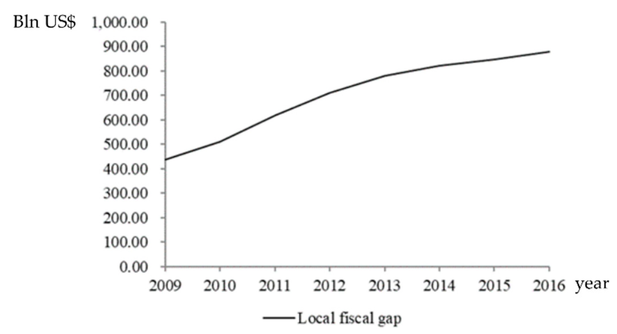
Figure 3.
The local government debt 2009–2016. Data source: Website of Ministry of Finance of People’s Republic of China.
Figure 3.
The local government debt 2009–2016. Data source: Website of Ministry of Finance of People’s Republic of China.


Table 1.
Changes of transferring area and revenue from land finance in recent years.
| (1) | (2) | (3) | (4) | (5) | (6) | (7) |
|---|---|---|---|---|---|---|
| Year | Transferring Area (000 ha) | Year-on-Year Change Rate of (2) % | Revenue from Land Finance (bln US$) | Year-on-Year Change Rate of (4) % | Local Fiscal Revenue (bln US$) | Proportion of Local Fiscal Revenue |
| 2010 | 291.50 | +32.00 | 309.38 | +108.45 | 429.70 | 0.72 |
| 2011 | 333.90 | +14.55 | 510.25 | +64.92 | 808.42 | 0.63 |
| 2012 | 322.80 | −3.32 | 437.27 | −14.30 | 939.65 | 0.47 |
| 2013 | 367.00 | +13.69 | 634.62 | +45.26 | 1061.07 | 0.59 |
| 2014 | 271.80 | −25.94 | 660.62 | +4.09 | 1167.09 | 0.57 |
| 2015 | 221.40 | −18.54 | 500.72 | −24.20 | 1292.06 | 0.39 |
| 2016 | 208.20 | −5.96 | 576.26 | +15.09 | 1341.46 | 0.43 |
Data source: Website of Ministry of Finance of People’s Republic of China.
Table 2.
The 41 major Chinese city governments.
| East region | Beijing, Tianjin, Shijiazhuang, Shenyang, Dalian, Shanghai, Nanjing, Suzhou, Wuxi, Hangzhou, Ningbo, Fuzhou, Xiamen, Quanzhou, Jinan, Qingdao, Guangzhou, Shenzhen, Dongguan, Foshan, and Haikou |
| Central region | Harbin, Changchun, Taiyuan, Hefei, Nanchang, Zhengzhou, Wuhan, and Changsha |
| West region | Chengdu, Chongqing, Guiyang, Kunming, Xi’an, Lanzhou, Xining, Lhasa, Yinchuan, Urumqi, Nanning, and Huhehot |
Table 3.
City governments’ main sources of revenue and expenditure.
| Revenue | Expenditure |
|---|---|
| 1.Tax revenue | 1. General public expenditure |
| 1.1 Value-added tax (VAT) * | 1.1 Public safety expenditure |
| 1.2 Sales tax | 1.2 Education expenditure |
| 1.3 Corporate income tax | 1.3 Science and technology expenditure |
| 1.4 Personal income tax | 1.4 Cultural, sports, and media expenditure |
| 1.5 Construction tax | 1.5 Medical and family planning expense |
| 1.6 Land value increment tax | 1.6 Energy saving and environmental protection expenditure |
| 1.7 Deed tax | 1.7 Agricultural and forestry expenditure |
| 1.8 Vehicle and vessel tax | 1.8 Resource exploration expenditure |
| 1.9 Stamp tax | 1.9 Land and sea meteorological expenses |
| 1.10 Other taxes | 1.10 Resident housing expenditure |
| 2. Non-tax revenue | 1.11 Cereals, oils, and other material reserves expenditure |
| 2.1 Administrative fee income | 1.12 Business service related expenditure |
| 2.2 Penalty and confiscatory income | 1.13 Transportation expenditure |
| 2.3 Lottery public welfare income | 1.14 Expenditure on urban infrastructure construction |
| 2.4 Port construction fee income | 1.14 Other general public expenditure |
| 2.5 Sewage treatment fee income | 2. Non-general public expenditure |
| 2.6 Land finance income | 2.1 Land finance related expenditure (e.g., payments for the transferring land, expenses for resettlement of peasants, and subsidies for the lost crops growing on transferring land) |
| 2.7 Vehicle toll income | 2.2 Debt repayment expenditure |
| 2.8 State-owned capital operating income | 2.3 Interest expenditure |
| 2.9 Other non-tax revenue | 2.4 State-owned capital operating related expenditure |
| 2.5 Other non-general public expenditure |
* Note: There are taxes that belong to both local and central government, such as VAT, the central government, and the LG each account for 50%.
Table 4.
Meaning and calculation of related variables.
| Variables | Meaning and Calculation |
|---|---|
| DEB | size of LG’s debt |
| LS | surplus of land finance, and land finance revenue minus land finance expenditure; land finance revenue refers to “land finance income (2.6)” in the left line of Table 3, land finance expenditure includes, in the right line of Table 3, “expenditure on urban infrastructure construction (1.14)”; “land finance related expenditure, for example, the payments for the transferring land; expenses for resettlement of peasants and subsidies for the lost crops growing on transferring land (2.1)”; “debt repayment expenditure (2.2)”; and “interest expenditure (2.3)”. |
| EX | basic fiscal expenditure, includes all the expenditures in the right line of Table 3 except the land finance expenditures listed above |
| RX | basic fiscal revenue, includes all the expenditures in the left line of Table 3 except the land finance income (2.6) |
| BS | basic budget surplus, basic fiscal revenue minus basic fiscal expenditure |
| r | average interest rate of government debt |
| g | economic growth rate |
| deb | size of debt/GDP |
| bs | the basic budget surplus/GDP |
| ls | the surplus of land finance/GDP |
| TR | transfer from higher governments |
| ND | increase in LG debt in a certain year |
Table 5.
Descriptive statistical analysis of related variables.
| Total Region | |||||||
| Variable | Mean | Median | Min | Max | P25 | P75 | SD |
| bs | −0.0713 | −0.0283 | −2.2300 | 0.0107 | −0.0482 | −0.0131 | 0.0261 |
| deb | 0.2616 | 0.2590 | −0.3280 | 0.7213 | 0.1481 | 0.3719 | 0.1581 |
| g | 0.1034 | 0.1021 | −0.2300 | 0.2265 | 0.0820 | 0.1250 | 0.0396 |
| ls | 0.0187 | 0.0114 | 0.0005 | 0.1185 | 0.0050 | 0.0242 | 0.0215 |
| Eastern Region | |||||||
| Variable | Mean | Median | Min | Max | P25 | P75 | SD |
| bs | −0.0180 | −0.0154 | −0.0576 | 0.0107 | −0.0278 | −0.0064 | 0.0168 |
| deb | 0.2277 | 0.2033 | −0.0608 | 0.6977 | 0.0960 | 0.3479 | 0.1583 |
| g | 0.0933 | 0.0920 | −0.2300 | 0.1750 | 0.0800 | 0.1170 | 0.0423 |
| ls | 0.0122 | 0.0058 | 0.0005 | 0.1009 | 0.0033 | 0.0145 | 0.0157 |
| Central Region | |||||||
| Variable | Mean | Median | Min | Max | P25 | P75 | SD |
| bs | −0.0355 | −0.0356 | −0.0734 | −0.0058 | −0.0492 | −0.0123 | 0.0187 |
| deb | 0.2892 | 0.2781 | −0.0037 | 0.5810 | 0.1861 | 0.3892 | 0.1265 |
| g | 0.1087 | 0.1065 | 0.0330 | 0.1750 | 0.092 | 0.1300 | 0.02834 |
| ls | 0.0231 | 0.0158 | 0.0033 | 0.1050 | 0.0094 | 0.0282 | 0.0206 |
| Western Region | |||||||
| Variable | Mean | Median | Min | Max | P25 | P75 | SD |
| bs | −0.1900 | −0.0525 | −2.230 | −0.0053 | −0.0934 | −0.0400 | 0.4642 |
| deb | 0.3030 | 0.2793 | −0.3280 | 0.7213 | 0.2114 | 0.3719 | 0.1651 |
| g | 0.1179 | 0.1192 | −0.0660 | 0.2265 | 0.0949 | 0.1400 | 0.0363 |
| ls | 0.0269 | 0.0161 | 0.0020 | 0.1185 | 0.0106 | 0.0303 | 0.0266 |
Table 6.
Estimated coefficients of the multiple regression model (cross-sectional data).
| Total Region | ||||||
| Independent Variable | c | bst−1 | deb | debt−1 | g | ls |
| Corresponding coefficient | ||||||
| Values of Coefficients | −0.0045 | 0.8989 | −0.1807 | 0.1785 | 0.0122 | −0.0049 |
| p Value | 0.055 | 0.000 | 0.000 | 0.000 | 0.036 | 0.070 |
| Eastern Region | ||||||
| Independent Variable | c | bst−1 | deb | debt−1 | g | ls |
| Corresponding coefficient | ||||||
| Values of Coefficients | −0.0090 | 0.9543 | −0.1334 | 0.1320 | 0.0671 | −0.0173 |
| p Value | 0.000 | 0.000 | 0.000 | 0.000 | 0.000 | 0.074 |
| Central Region | ||||||
| Independent Variable | c | bst−1 | deb | debt−1 | g | ls |
| Corresponding coefficient | ||||||
| Values of Coefficients | −0.0082 | 0.7859 | −0.1510 | 0.1392 | 0.0466 | −0.1174 |
| p Value | 0.027 | 0.000 | 0.053 | 0.056 | 0.000 | 0.026 |
| Western Region | ||||||
| Independent Variable | c | bst−1 | deb | debt−1 | g | ls |
| Corresponding coefficient | ||||||
| Values of Coefficients | −0.0079 | 0.8831 | −0.1591 | 0.1557 | 0.0577 | 0.0365 |
| p Value | 0.059 | 0.000 | 0.004 | 0.002 | 0.060 | 0.082 |
Table 7.
Estimated coefficients of the multiple regression model (panel data).
| Total Region | ||||||
| Independent Variable | c | bst−1 | deb | debt−1 | g | ls |
| Corresponding coefficient | ||||||
| Values of Coefficients | −0.0058 | 0.8945 | −0.1843 | 0.1803 | 0.0146 | −0.0061 |
| p Value | 0.025 | 0.000 | 0.000 | 0.000 | 0.036 | −0.034 |
| Eastern Region | ||||||
| Independent Variable | c | bst−1 | deb | debt−1 | g | ls |
| Corresponding coefficient | ||||||
| Values of Coefficients | −0.0073 | 0.9431 | −0.1408 | 0.1392 | 0.0588 | −0.0192 |
| p Value | 0.000 | 0.000 | 0.000 | 0.000 | 0.000 | 0.013 |
| Central Region | ||||||
| Independent Variable | c | bst−1 | deb | debt−1 | g | ls |
| Corresponding coefficient | ||||||
| Values of Coefficients | −0.0095 | 0.8623 | −0.1455 | 0.1403 | 0.0512 | −0.1158 |
| p Value | 0.000 | 0.000 | 0.037 | 0.028 | 0.000 | 0.017 |
| Western Region | ||||||
| Independent Variable | c | bst−1 | deb | debt−1 | g | ls |
| Corresponding coefficient | ||||||
| Values of Coefficients | −0.0067 | 0.8960 | −0.1605 | 0.1566 | 0.0485 | 0.0452 |
| p Value | 0.014 | 0.000 | 0.000 | 0.000 | 0.037 | 0.059 |
Table 8.
Descriptive statistical analysis of relevant variables.
| Variables | Mean | Median | Min | Max | SD |
|---|---|---|---|---|---|
| deb | 0.2616 | 0.2590 | −0.3280 | 0.7213 | 0.1581 |
| deb2 | 0.0870 | 0.0637 | 0.0001 | 0.5203 | 0.0914 |
| ln(GDP/Population) | 8.3522 | 8.2056 | 7.5819 | 12.0362 | 0.9820 |
| CPI | 0.0426 | 0.0405 | −0.0318 | 0.1760 | 0.0377 |
| ls | 0.0187 | 0.0114 | 0.0005 | 0.1185 | 0.0215 |
| g | 0.1034 | 0.1021 | −0.2300 | 0.2265 | 0.0396 |
Table 9.
Empirical results of the model (16).
| Variables | Cross-Sectional Data Model | Panel Data Model |
|---|---|---|
| C | 0.0428 *** | 0.0509 *** |
| (7.092) | (6.670) | |
| deb | 0.0061 ** | 0.0053 * |
| (2.054) | (1.847) | |
| deb2 | −0.0054 * | −0.0049 * |
| (−1.746) | (−1.821) | |
| ln(GDP/Population) | 0.0068 *** | 0.0035 *** |
| (4.149) | (3.116) | |
| CPI | 0.0214 ** | 0.0308 ** |
| (2.106) | (2.215) | |
| ls | 0.0034 | 0.0029 |
| (1.277) | (1.503) | |
| gt−1 | 0.0761 *** | 0.0525 *** |
| (3.540) | (4.182) | |
| Reg/Year | NO | YES |
| R2 | 0.372 | 0.304 |
| F value | 27.034 *** | 26.520 *** |
| N | 287 | 287 |
Note: * = significant at 10%; ** = significant at 5%; *** = significant at 1%.
© 2018 by the authors. Licensee MDPI, Basel, Switzerland. This article is an open access article distributed under the terms and conditions of the Creative Commons Attribution (CC BY) license (http://creativecommons.org/licenses/by/4.0/).
Share and Cite
MDPI and ACS Style
Tu, L.; Padovani, E. A Research on the Debt Sustainability of China’s Major City Governments in Post-Land Finance Era. Sustainability 2018, 10, 1606. https://doi.org/10.3390/su10051606
AMA Style
Tu L, Padovani E. A Research on the Debt Sustainability of China’s Major City Governments in Post-Land Finance Era. Sustainability. 2018; 10(5):1606. https://doi.org/10.3390/su10051606
Chicago/Turabian StyleTu, Lihe, and Emanuele Padovani. 2018. "A Research on the Debt Sustainability of China’s Major City Governments in Post-Land Finance Era" Sustainability 10, no. 5: 1606. https://doi.org/10.3390/su10051606
Note that from the first issue of 2016, this journal uses article numbers instead of page numbers. See further details here.