Article

A Comparison of Vacancy Dynamics between Growing and Shrinking Cities Using the Land Transformation Model

1
Department of Urban Design and Planning, Hongik University, Seoul 04066, Korea
2
Department of Landscape Architecture and Urban Planning, Texas A&M University, College Station, TX 77843, USA
3
Architectural and Urban System Engineering, Ewha Womans University, Seoul 03760, Korea
*
Author to whom correspondence should be addressed.
Sustainability 2018, 10(5), 1513; https://doi.org/10.3390/su10051513
Submission received: 14 April 2018 / Revised: 4 May 2018 / Accepted: 8 May 2018 / Published: 10 May 2018
(This article belongs to the Section Sustainable Urban and Rural Development)

Abstract

:
Every city seeks opportunities to spur economic developments and, depending on its type, vacant land can be seen as a potential threat or an opportunity to achieve these developments. Although vacant land exists in all cities, the causes and effects of changes in vacant land can differ. Growing cities may have more vacant land than shrinking cities because of large scale annexation. Meanwhile, depopulation and economic downturn may increase the total amount of vacant and abandoned properties. Despite various causes of increase and decrease of vacant land, the ability to predict future vacancy patterns—where future vacant parcels may occur—could be a critical test to set up appropriate development strategies and land use policies, especially in shrinking cities, to manage urban decline and regeneration efforts more wisely. This study compares current and future vacancy patterns of a growing city (Fort Worth, TX, USA) and a shrinking city (Chicago, IL, USA), by employing the Land Transformation Model (LTM) to predict for future vacant lands. This research predicts and produces possible vacancy pattern scenarios by 2020 and deciphers the ranking of determinants of vacant land in each city type. The outcomes of this study indicate that the LTM can be useful for simulating vacancy patterns and the causes of vacancy vary in both growing and shrinking cities. Socio-economic factors such as unemployment rate and household income are powerful determinants of vacancy in a growing city, while physical and transportation-related conditions such as proximity to highways, vehicle accessibility, or building conditions show a stronger influence on increasing vacant land in a shrinking city.

Graphical Abstract

1. Introduction

Many countries have experienced large waves of urban growth, globally [1]. The United Nations (2013) projects the world will add 2.3 billion more people by 2050 with the population reaching 9.8 billion; the proportion of urban populations will rise from 3.6 to 6.3 billion, which accounts nearly 67% of the world’s population [1,2]. However, population increases are not distributed equally among all cities. Several developed countries including Germany and Japan have experienced stagnant population growth in many large cities while other cities in developing countries such as China and India are growing rapidly, resulting in an uneven population distribution. For example, Japan’s top 10 cities lost 12.9% of total population between 1990 and 2007. This is a relatively large loss when compared to the overall population change of −1.01% across Japan [3]. Meanwhile, the 2010 Census revealed that the total population of Beijing increased by 44% over the last decade, a considerably large number when considering the average population growth in 1990 was 1.5%, 0.8% in 2000, and 0.5% in 2010 [4]. Deindustrialization, globalization, urban decentralization, suburbanization, and changing household demographics are typically listed as the main drivers of fluxes in population [5]. Depopulating cities mostly struggle from socio-economic declines, decreased tax revenue, and increased vacant land/abandoned structures. As Bowman and Pagano (2004) mentioned [6], vacant land is not always bad. Temporal vacant patterns can be observed as a part of industrial restructuring process from manufacturing to service; or it can be seen as potential resource for future development or habitat. Inversely, an excess of abandoned structures or underutilized land could possibly cause economic, social and environmental problems such as urban disinvestment, reduced tax revenues, overburdened social programs, increased stock of vacant housing, and increased crime and poverty [7]. As such, forecasting future vacant land dynamics can be socially, physically and environmentally beneficial for both growing and shrinking cities and is critical first step to develop proactive land use policies [6,8,9] in an effort to not waste public funds to operate or maintain under- or unused facilities and public services. Due to technological constraints and time limits, unfortunately, few academic studies and planning practices seek to advance land use prediction modeling, especially in regard to vacant properties.
To fill this gap, this research attempts to develop urban vacancy prediction scenarios using The Land Transformation Model (LTM) and eighteen determinants of vacant land prediction [10]. The LTM is a land use prediction tool that is operated by artificial neural networks (ANNs) through Geographic Information Systems (GIS). Using the 1990 and 2000 data, LTM produced 2020 vacant land prediction scenarios and the level of accuracy assessment tests were also performed. In particular, this research attempts to explore which factors contribute to creating vacant land and the degree of influence of these determinants in two different types of cities: shrinking and growing. In terms of defining growing and shrinking cities, population, employment growth, or age distribution are well-known critical factors to analyze the patterns of city growth trends. This research only highlights the population change to define growing and shrinking cities. Shrinking cities are cities losing population and growing are gaining in population. Chicago, IL, USA was chosen as a study area to represent a shrinking city, while Fort Worth, TX, USA is used to represent a growing city. The outcomes of this study are expected to guide well-informed policies for vacant properties and be utilized by planners and policy makers in charge and used as a rationale to cope with temporal and chronic vacancy issues, and consequently, the accurate prediction model can contribute to a successful and sustainable urban environment.

2. Literature Review

2.1. Growing Cities, Shrinking Cities, and Vacant Land

There are various ways to define growing and shrinking cities, but most definitions are based on the demographic, physical, social, and economic conditions of municipalities. Growing cities are often recognized as cities with a rapid population increase and economic intensification [11,12,13]. In these cities, economic growth typically increases the demand and supply in both workers and consumers, resulting in accompanied population growth and housing, infrastructure, and public service needs. The U.S Census Bureau and the Brookings Institution also listed the fastest growing cities based on population and employment growth data.
Like growing cities, population is the most popular criteria to identify a shrinking city. While depopulation alone does not always necessarily mean a city is declining, this condition can often act as a catalyst for urban decline and socio-economic shifts. Schilling and Logan (2008) defined a shrinking city as older industrial city losing more than 25% in population over the last 40 years [14]. Reckien and Martinez-Fernandez (2011) define shrinking cities as urban areas that have experienced depopulation, employment loss or/and economic downturns over the past 40–50 years [15]. In 2004, the Shrinking Cities International Research Network (SCIRN) was launched at the instigation of the University of California, Berkeley and highlighted the combination of population and economic decline simultaneously. They defined a shrinking city as an urban area with more than 10,000 residents that have experienced depopulation for more than two years resulting in economic crisis [16].
Massively shrinking cities are often accompanied by physical decay. Therefore, increased vacancies and abandonment is typically an issue related to urban shrinkage. Property owners of vacant structures are likely to neglect up-keeping efforts of ownership such as paying taxes, paying utility bills, maintaining yards, or fixing housing structures over the years [17]. These abandoned and neglected sites can also be catalysts for eventual increases in criminal activity [18]. Neighborhoods with a large amount of unoccupied lots may have difficulty in re-selling nested properties because their market values are often depreciated. This causes a decrease in tax revenues for municipalities, typically resulting in lower support for public improvements and maintenance. As a consequence, more people leave the city.
It is important to note the difference in vacant land types across cities. Vacant land does not only include brown or grayfields with lower levels of occupancy. It can also be developable greenfields or simply empty or underperforming areas; some municipalities even classify agricultural or recreational land as vacant. A survey on vacant land amounts by Newman et al. (2016) showed green spaces be the most common type [10]. Greenfields (61.9%), unused agricultural lands (49.2%), brownfields (47.6%) and derelict open space (33.3%) rounded out the top 5 listed types of vacant lands. Regionally, Southern cities had a higher preponderance of unused agricultural lands, while Midwestern cities reported a greater prevalence of brownfields. Given this situation, vacant land can be either a good or bad, depending on the type. Some types of vacant land can remain as unused for future developments, provide habitat for ecosystems, or can provide green space for residents. Insufficient vacant land in rapidly growing cities can limit the expansion of cities. Inversely, if a city has overwhelming amounts of abandoned structures, it will tend to indicate long cycles of shrinkage. Therefore, one of the primary planning goals of shrinking cities is how to convert vacant properties into valued community assets and how to effectively manage vacant land supplies. New technologies have significantly aided in this plight.

2.2. Historical Urban Land Use Change Models

As computer systems and federal data organizations in the late 1950s and mid-1960s were developed, urban growth and land use change models emerged to help manage future growth [19]. Most land use change models were initially developed to predict the economic and environmental impacts of land-use transportation policies. In 1959, basic gravity models were employed to investigate the attractiveness and accessibility of cities in metropolitan areas for future development [20]. Lowry (1964) also applied a transportation model to allocate future residential and service employment zones based on the analysis of travel costs and attractiveness of in the Pittsburgh region [21]. Econometric models are the most common statistical technique, using multiple regression analysis. After Swerdloff and Stowers integrated statistical techniques into prediction modeling in 1966 [22], Chapin and Weiss introduced a probabilistic model of residential growth in 1968, and statistical models are still employed in several related current studies [23]. Statistical models were employed to analyze the problems involving economic demand and supply, but the application of these techniques proved useful in analyzing the relationship between the distribution of land use types and other driving factors and estimating the layout of urban land uses based on principle of economic/market equilibrium [23]. However, these traditional econometric models were criticized because the modeling processes were too static; aggregated macro-scale data were used due to the limitation of data collection and technology [24]. Since the statistics-based models basically assumed long term, linear relationships and temporal stationarity, it was restrictive to apply the models to real conditions. In order to assuage this condition, different empirical models such as non-linear statistical methods and artificial neural networks were coupled with advanced computing abilities.

2.3. The Land Transformation Model (LTM)

The regression models focus on identifying functional relationships between spatial input factors and input patterns [25]. More recently, in an effort to solve many urban issues, planners have slowly moved into spatial and temporal models which produce realistic landscape patterns more scientifically and technologically. UrbanSim [26], Cellular Automata models [27,28] and SLEUTH [29] have remarkably grown in the last 30 years [10]. Since these models simulate transitions using spatially explicit digital maps, graphical outputs can be provided, and they rely not only on economic theories, but also reflect real situations and historical urban trends. Recently, land use and cover change (LUCC) models comprised of Geographic Information Systems (GIS) and artificial neural networks (ANNs) such as the LTM, have grown in popularity to analyze spatio-temporal land use changes, estimate the impacts of urban growth alterations and forecast land use changes [10,30]. Through a preprocessing process with GIS tools, historical spatial data layers are controlled managed, while, ANNs learn about input patterns (historical land use dynamics) and influential drivers (input factors) [31,32]. While most computer modeling tools focus on regional scales analyses, there is a lack of local scaled predictions using the LTM and testing of the overall accuracy of created models has not been thoroughly conducted in many studies. Although many other computer-based models are based on similar processes and concepts, one great asset of the LTM is that it displays the accuracy of the model while other models typically simply specify whether inputted drivers or factors have a significant effect on urban growth.

3. Literature Gaps and Research Objective

The multiple studies conducted on urban shrinkage in the last fifty years have strongly connected it to urban decline, structural deterioration and physical decay, employment loss, and social exclusion [14,33,34,35,36,37,38]. The existing research, however, has not been successful to differentiate vacant land conditions between growing and shrinking cities, nor is there a thorough body of knowledge examining causal factors contributing to vacancies in either city type. First, most studies have focused on demographic and economic aspects such as population changes and unemployment rate as the primary factors increased vacant lands. However, as noted, vacant properties are actually more numerous in growing cities than shrinking [36]. As Lang mentioned, “just because a city has fewer residents and fewer jobs does not mean that it is experiencing decline; the issue is the composition of those changes, their pace and the resultant distribution of costs and benefits” ([39], p. 2). The problem of population loss is not about amount, but about who is leaving and who is staying. While some research has examined how socio-economic status changes in a declining city, it is difficult to find much literature on the relationships between a mix of physical, social, and economic characteristics and vacant land. While most of the studies describe the demographic trends of a region, only a small number of existing studies attempt to assess the statistical significance of those factors. Based on the literature, 18 primary driving factors can be the principal causal mechanisms explaining vacancy dynamics.
In terms of computer modeling tools, LUCC models have altered drastically over the last 50 years and machine learning has increased their reliability. However, most urban spatial prediction models have focused on regional scaled analyses, primarily concentrating on the impacts of urban development patterns on natural resources. Since municipal scaled predictions are rare and a model for predicting vacant urban land has only recently been developed in 2016, more applications and testing of this model are needed [1]. Newman et al. (2016) and Lee and Newman (2017) predicted future possible vacancy dynamics using the LTM, but focused only on model development, calibration methods, and accuracy assessment, not the comparison of the main determinants of vacancy [1,10]. This paper seeks to apply the vacant land model using the LTM to (1) to project possible future vacancy pattern scenarios (2) rank the effect of determinants of vacant land and (3) to compare the differences of influences of vacancy in growing and shrinking cities to establish well-informed policies on the appropriate uses of vacant properties.

4. Methods

4.1. Study Area

In order to observe the difference of urban vacancy patterns between growing and shrinking cities, 62 cities with a population over 250,000 as of 2000 in the United States were sorted then the most populating and depopulating cities were identified; Honolulu, HI is excluded in the analysis. Of these cities, from 2000 to 2010, Fort Worth, TX increased in population the most, 206,512 (+39%), while the city of Detroit, MI lost −237,493 people (−25%) as shown in Table 1. However, Chicago, IL, who ranked in 2nd in most depopulation cities, was chosen as a representative of shrinking cities since decline-related issues of Chicago have tended to be relatively underestimated compared to other declining cities such as Detroit, Cleveland, and Cincinnati.

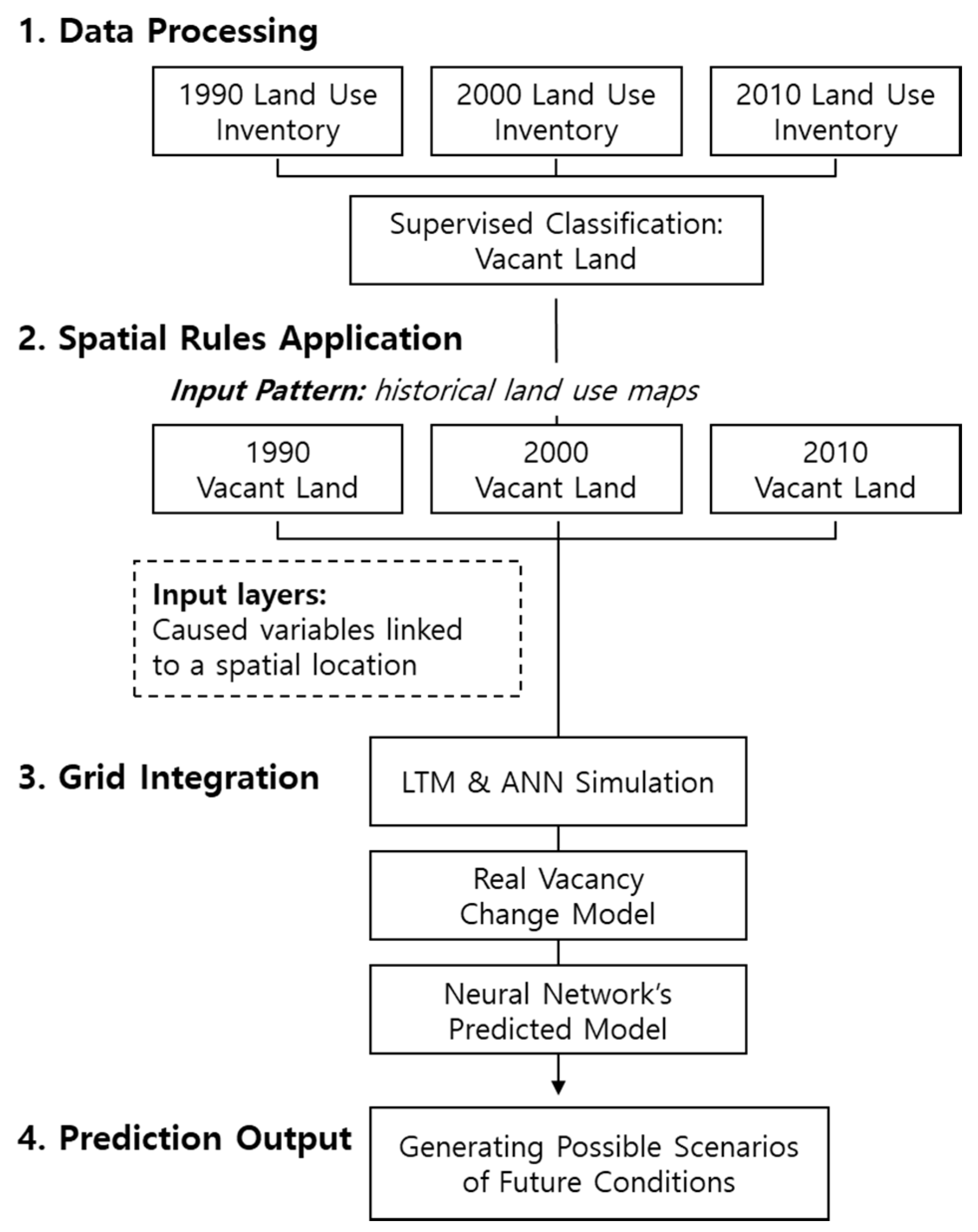
4.2. Model Specification: The Land Transformation Model (LTM)

The LTM is capable of analyzing spatial and temporal land use dynamics as well as estimating the impacts of urban growth alterations to forecast land use changes [29]. The LTM adapts based on the land use/cover change (LUCC) through GIS and ANNs. Although other computer-based models exist based on similar processes and concepts, one great asset of the LTM is a capability of quantifying the effect of each factor through model performance.
The LTM is processed by following four sequential steps (see Figure 1). First, spatial input layers integrated with GIS are generated, stored and managed. GIS is used to quantify historical temporal changes in spatial patterns and forecast future possible scenarios. The grid cells of base input layers represent land use as binary (presence = 1 or absence = 0; in this study, vacant land = 1 or occupied land = 0). Second, the predictor variables are reclassified from the input layers based on two different transition rules in ANNs: patch size and distance from the location of a predictor cell. Since socioeconomic variables can be obtained by census boundary (e.g., census tracts or block groups), the variable values of all cells within the defined patches are same. The Euclidian distance formula is used to calculate the values of transportation/street-related variables as a tool of the distance spatial transition rule. Third, grid integration allows the ANN to learn about input layers—which are driving factors—and output data–which refer to historical land use change patterns. There are three major integration strategies such as ANNs, multi-criteria evaluation (MCE), and logistic regression (LR). Each method requires a different data normalization process and there are various ways of defining the transition rules and model structures. In this research, all cell sizes and an analysis window are set to a fixed base layer by ANNs to provide a simulation environment using a gridded space (raster). Lastly, temporal scaling of prediction output through a “principal index driver” (PID) is used to determine how much land is expected to transit over a given time period. The existing literature assumes that the transitioned number of cells will increase the same proportion based on the analysis of historical temporal and spatial land use data [40]. This study also considers historical population growth statistics and future projection to calculate the PID. By using both land use and population data, it is possible to obtain more reliable future possible scenarios.
For example, the LTM firstly identifies the change of vacant patterns from 2000 to 2010 and also predicts 2010 vacancy pattern using 18 determinants of 2000. Then it compares the actual and projected 2010 urban vacancy pattern and adjust the weighting of each driving factor. The ANN repeatedly runs until it can produce the same result of the actual 2010 patterns. Based on the weights learned from 2000 to 2010, the model can project change by 2020. The time period can be changed by the research interests.

4.3. Variable and Data

Because variable selection greatly affects prediction outcomes, identification of factors that determine vacant land formation is a critical task to increase the accuracy of the model. Previous studies were carefully observed, and major four constructs were set as below. Due to these factors, an oversupply of vacant land can hinder residential, commercial and business activities in an entire city, and consequently, can contribute a decrease in land prices, property values and tax revenues [14,41].
  • Employment Trend: deindustrialization or shifts from an industrial to service economy [42,43,44,45];
  • Socio-economic Status: decreasing personal wealth [46,47,48,49];
  • Household/Housing: weak market conditions and downturns [49,50,51]; and
  • Physical Conditions and Accessibility: odd physical characteristics/location [44,47,52].
Under these four constructs, this research used three different types of input drivers to forecast 2020 vacancy patterns and quantify the influences of each factor: (1) influential variables linked to a spatial location (referred to as input factors), (2) historical vacant land use inventories between 2000 and 2010 (referred to as input patterns, and (3) exclusionary layers which were omitted from the analysis due to their specialized functionality (i.e., military bases, airports, public facilities, parks and open space and existing vacant areas). 18 related input factors were selected and measured as shown in Table 2. These 18 variables were limited by the data availability so that 15 variables for Fort Worth were utilized and 18 variables were used for Chicago to predict 2020 possible vacancy scenarios. Most socioeconomic variables were collected at the census block group level retrieved from the U.S. Census Bureau and other parcel–level data such as parcel size and transportation data (proximity to highways and railroads) were retrieved from North Central Texas Council and Chicago Metropolitan Agency. Then, all of input patterns and driving factors of vacant land was converted as raster data with a resolution of 100 by 100 feet.

4.4. Model Reliability and Accuracy

Although LTM usage has risen in popularity, the model been criticized for not always being able to provide proof of highly accurate outputs due to ineffective assessment processes during the research process [53]. Due to this issue, it can be difficult to calibrate the contribution of these models, making the prediction output are difficult to adapt to local circumstances and communities [19]. Thus, it is critical to improve the model’s reliability by proven assessment processes and develop an acceptable model.
There are a few accepted methods to validate a model’s performance. For model calibration, the goodness of fit of the neural network-based model was verified using four different sets of metrics such as (1) Kappa coefficients, (2) percent correct metric (PCM), (3) agreement/disagreement measures, and (4) the relative operating characteristic (ROC), comparing the cell locations between real change and predicted change over a given time frames.
Since spatially-explicit LUCC models require a set of digital maps over at least two time periods and then simulate transitions to produce a prediction map for a subsequent time [54], over 4000 cycles of training are typically required to stabilize the error level to a minimum in the ANN [1]. Also, each training session for this research was run to 250,000 cycles as the best output could be possibly obtained with more than 250,000 cycles of training [55]. As a result of the neural network training, two automated statistics, Kappa values and PCM were calculated every 1000 cycles. Finally, a pair of maps from actual change and simulated model with the highest match rate was selected.
Among the accuracy assessment processes, Kappa analysis has, for a long period, been a standard component in the conduction of accuracy assessments [56]. As Congalton and Green stated [57], “Kappa analysis has become a standard component of most every accuracy assessment and is considered a required component of most image analysis software packages include accuracy assessment procedures” ([58], p. 4408). This accuracy assessment can be simply computed and easily understood and interpreted. The Kappa statistic is calculated to measure the agreement between how much agreement is actually present from an actual transition map compared to how much agreement would be expected from a predicted transition map. Since the value is standardized to lie on a 0 to 1 scale showing degree of agreement, the Kappa value can be interpreted the same across multiple studies [59]. A value of 1 implies perfect agreement, exactly what would be expected by chance for 0, less than change agreement would equate to a negative value. Generally, values fall between 0.01 and 0.20 indicate no or slight agreement and fair agreement ranges between 0.21and 0.40. The value of 0.41 to 0.60 is considered to be moderately, from 0.61 to 0.80 as substantially, and from 0.81 to 1.00 as almost perfectly agreed status [60,61,62,63]. Since land use maps are categorical datasets, Kappa analysis is frequently used to compute the agreement between a pair of maps.
Nevertheless, due to the conceptual problems and methodological flaws of the Kappa, the use of only Kappa has shown somewhat limited. Since the Kappa score is a one-dimensional index, the value of Kappa is not always successful to evaluate both quantity and location accuracy with a high level of certainty in grid cells among the utilized maps [1,64]. Further, the Kappa index is able to muddle information of the quantity of each category on the maps with the locational information of each category on the map. Therefore, the quantity and allocation disagreement from a general map comparison can provide additional insights [10,65].
The assessment process of PCM is relatively similar to the process of allocation disagreement. While allocation disagreement shows the overall proportion of misallocated pixels including zero value pixels, PCM focuses on the transited pixels having one or two values. Since the value of PCM indicates the proportion of pixels that transition, it is used to understand the transition of the land-cover category under investigation. Generally, the PCM result is interpreted as follows: values between 60% to 80% accuracy indicate an exceptional model and 40% to 60% are acceptable models [60,61,62,63].
Lastly, the receiver operating characteristic (ROC) curve analysis was employed as a quantitative measure to validate the goodness of fit of the LUCC model [66,67,68]. The two-class (binary classification) prediction model has four different outcomes such as True Positive (TP), False Positive (FP), True Negative (TN), and False Negative (FN). Using these four values, the sensitivity—true positive rate—and specificity—true negative rate—is calculated based on the overall agreement cell score outputs. Then, the sensitivity of ROC curve graphs on the x on the y-axis against 1-specificity—axis, and the area under the ROC curve (AUC) graphically displays the overall accuracy. Values that range between 0.70 and 0.79 indicate a fair fit, from 0.80 to 0.89 substantial, and from 0.90 to 0.99 as excellent (1.0 is perfect) [69,70].

5. Results

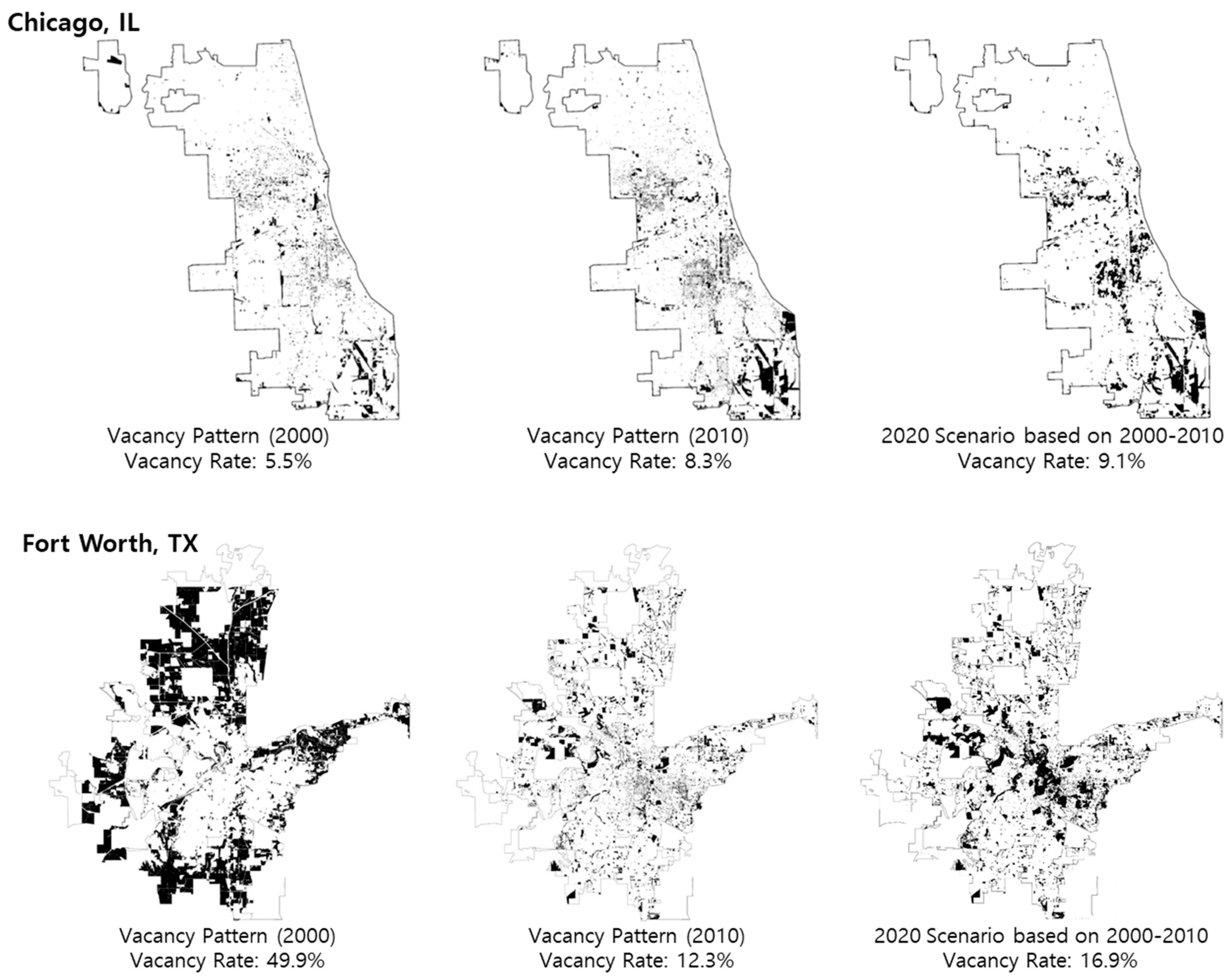
5.1. Possible Scenarios of Vacancy Patterns by 2020 and LTM Output Statistics

The City of Fort Worth (2014) categorizes vacant land into three different: vacant brownfields, vacant structures and housing units, and vacant agricultural land. According to the city’s definition, vacant brownfields are industrial or commercial properties where redevelopments are typically burdened by real or perceived contamination so that the area underutilized and structurally degraded. Vacant structure and housing units include vacant buildings such as houses, apartments, mobile homes or similar. Vacant agricultural land is an area with a lower density (i.e., one unit per acre) with limited infrastructure (e.g., water or sewer) or without any buildings, except for living quarters for mining, farming or grazing activities.
The City of Chicago describes vacant land differently. Vacant land is “land in an undeveloped state, with no agricultural activities nor protection as open space” [71]. Vacant land is grouped into four different classifications: brownfields, vacant structures/housing units, under development/construction and vacant forested, grassland and wetlands. The definition of vacant brownfields from Fort Worth and Chicago is same. Vacant structures/housing units contain undeveloped residential, commercial or industrial land appraised by the county assessors. Under development/construction land is an area with incomplete construction activities (e.g., roadway begun, partially-completed structures, missing or incomplete landscaping), which are identified by observation of aerial imagery. Lastly, vacant forested, grassland and wetlands refer to grassland or wetlands that exceed 2.5 acres. Unfortunately, despite the differences in vacant land classification, there is no way to separate the data in each classified vacant land type with existing available data. Each data file was released by simply labeled as vacant or non-vacant.
Figure 2 shows historical vacant land pattern changes and ratios of vacant land in Fort Worth and Chicago between 2000 and 2010 in 10-year increments (input patterns), and a possible 2020 vacant land scenario using the LTM output. In the 1990s, large scale annexation increased the total vacant land by 50% in Fort Worth, but the annexed vacant parcels rapidly decreased by about 12% in 2010 due to new developments occurring on the periphery of city. In contrast, Chicago‘s total amount of vacant land had slightly decreased from 5.9% to 5.1% between 1990 and 2000 since the population of the city somewhat stabilized in that time period. However, as with many older industrial cities in the U.S, the national foreclosure crisis in 2008 and depopulation trends by deindustrialization of Chicago have also resulted in increased vacant lots and abandoned lots in recent years.
In order to minimize the error level and get the best output in the ANN, each model had over 250,000 cycles of training sessions and the results of four statistics were used to compare actual vacancy rates and predict vacancy rates using 10-year period input patterns and input factors (See Table 3). Results for all comparisons of both cities yielded high enough statistics to merit acceptability of all predictions based on all accuracy assessment methods.

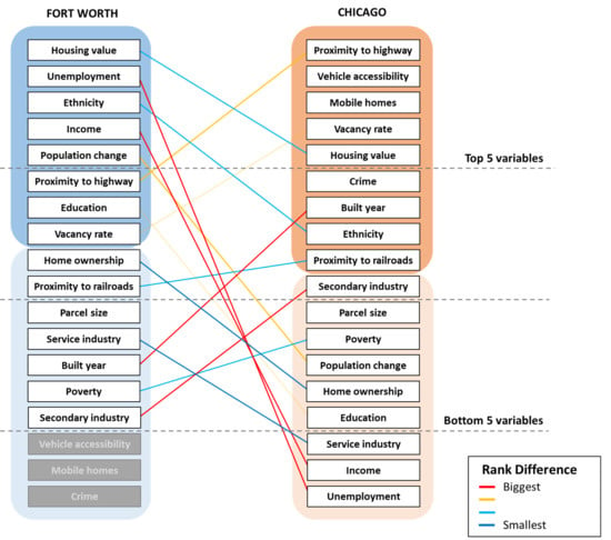
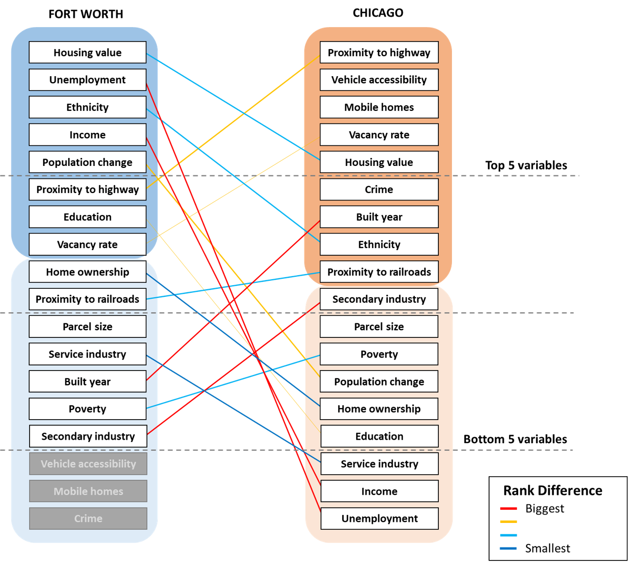
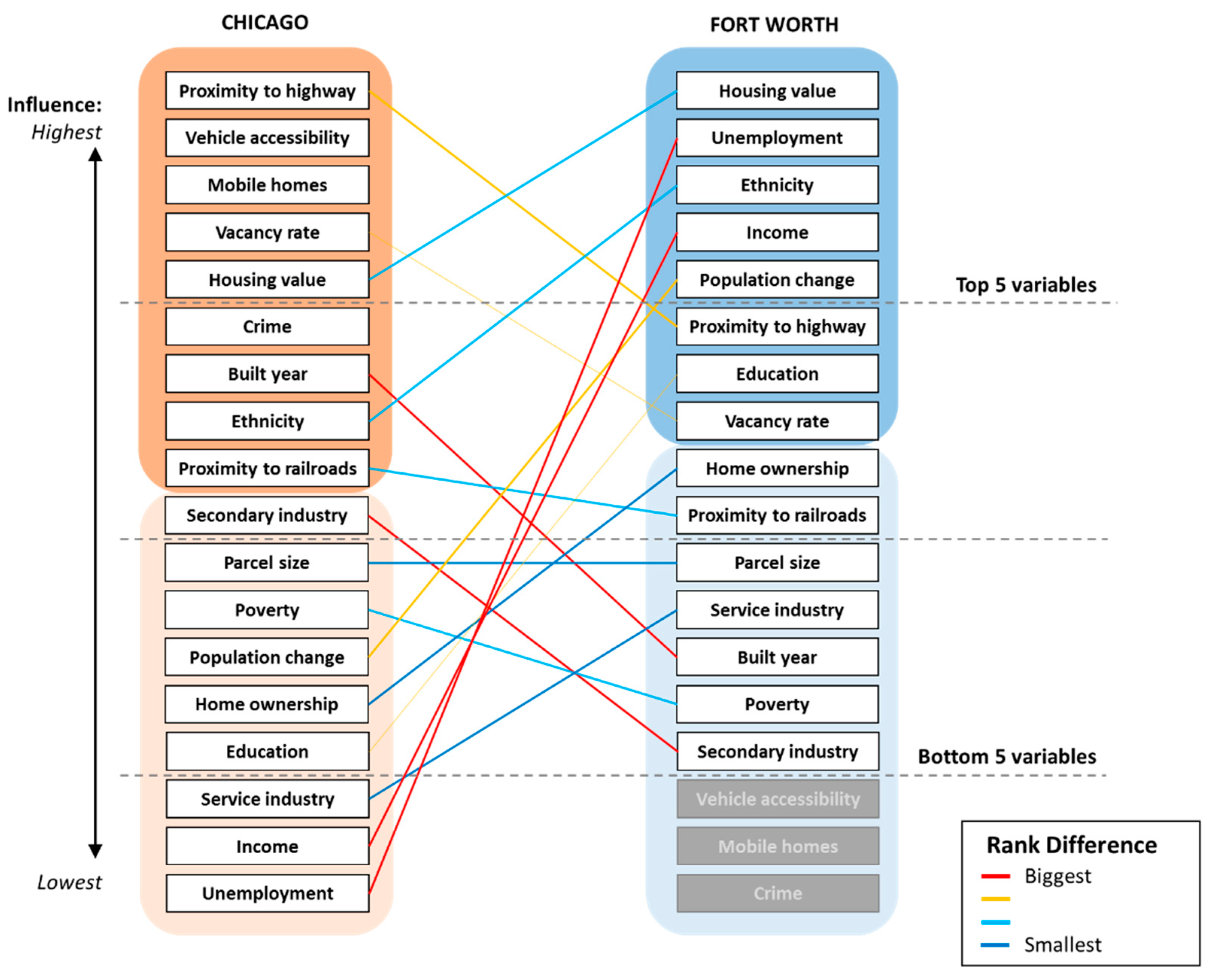
5.2. Influence of Vacancy Determinants in Two Types of Cities

As shown in Table 4, comparing the statistical output to the full model results, when dropping the rate of secondary industry (proportion of secondary industry employees to all industries), the model produces a higher PCM and Kappa than the full model, meaning that the factor may not be a strong influence to predict vacant land in Fort Worth. Since existing manufacturing and construction industries in a growing city may not be deindustrialization, this factor may be more powerful and influential in legacy or shrinking cities experiencing depopulation and deindustrialization. In contrast, market conditions and socio-economic variables such as housing value and unemployment rate seemed to be more influential compared to other factors; PCM and Kappa statistics decreased immensely when they were removed. Surprisingly, population change was not found as the most influential factor in predicting vacant land, while other demographic variables such as ethnicity (non-white population rate) and personal income were actually more influential on increasing prediction accuracy than simple population change. Physical and locational characteristic variables such as age of buildings and vehicle accessibility had weak but positive influences. Not surprisingly, proximity to highways proved to be a stronger impact than the proximity to railways.
In Chicago, all eighteen factors show an influence on vacancy pattern changes. When dropping the proximity to highway and vehicle accessibility measured by percent of households with no vehicle available, the model produces the lowest PCM and Kappa value, indicating that transportation and accessibility-related factors had a stronger influence on the model than other factors. Further, housing-related variables including housing value and mobile home rate also showed a stronger influence on increasing vacant land, while personal wealth variables such as income, unemployment rate and educational attainment seemed to be weak determinants. Since Chicago suffered more serious shrinkage issues in the 1960s and 1970s, rapid population changes may have already occurred during that time period. Thus, these factors may be more powerful and influential in cities which have experienced depopulation and deindustrialization recently or in fast growing cities.
The results of influence test indicate that market condition and accessibility such as housing value and proximity to highway are strong predictors of vacant land in both Chicago and Fort Worth (See Table 4 and Figure 3). It is well known the fact that better access to transportation is often considered as an amenity and contributes to increase neighborhood satisfaction [72,73,74]. Also, housing price is a strong indicator of neighborhood satisfaction; the higher the price, the higher the neighborhood satisfaction [75]. As such, a neighborhood with a lower neighborhood quality is more likely to experience more resident’s migration resulting in more vacancy. Is it important to note that not only do types of vacant properties change per city type, but the influence of each factor, and therefore the determinants of vacant property, are different in growing and shrinking cities.
In contrast to findings of previous literature, unemployment rate, income, and ethnicity were less critical factors on urban vacancy in shrinking cities, but those factors are shown as important in growing cities. This may be because Chicago has experienced serious depopulation and economic downturn over the past 60 years, with population movement stabilizing only recently. On the other hand, Chicago may face a deeper problem of increasing economic segregation and rapid demographic changes, leading to a growing amount of vacancy in declining neighborhoods. Inversely, small parcel size and low home ownership rate seemed to have a weak influence on vacancy prediction.
Not surprisingly, secondary industry appeared to be more influential in Chicago where many existing manufacturing industries have been deindustrializing than in Fort Worth, while service industry (proportion of service industry to all industries) proved to be less influential than secondary industry in predicting vacant land in both cities. This may be because continuous deindustrialization of manufacturing industries may influence depopulation and increase vacant land more strongly shrinking cities. However, the statistical outputs suggest that secondary industry is influential, though only marginally. Since the mass deindustrialization of Chicago began from the 1960s into the 1980s, secondary industry may be more influential if the variable influence test was conducted using input drivers in the 1960s or 70s.
Poverty rate also had a stronger influence in Chicago than Fort Worth. Since depopulating and deindustrializing neighborhoods with higher poverty rates typically have a lower potential future economic growth, increased poverty is related to joblessness, and can therefore contribute to depopulation.

6. Discussion

This research sought to use a proven land use prediction model to simulate vacant land changes in shrinking and growing cities in order to differentiate causal predictive factors for reach city type. To summarize findings from observations and analyses, several interesting trends were revealed. First, the LTM has shown that both Fort Worth and Chicago scenarios in this study have sufficiently high accuracy outputs to merit the acceptability of predictions. To minimize the error and produce the best result, more than 250,000 cycles of trainings were performed for each model and the results of four statistics were used to compare actual vacancy rates and predict vacancy rates using 10-year input patterns and input factors. Results for all comparisons of both cities produced acceptable statistics to merit the acceptability of predictions. Each model has high enough Kappa coefficients and PCM’s (40% or more) with fair to good AUC outputs (between 0.70 and 0.80) and thus, all models have high level of agreement.
Second, the variable influence test outputs indicate that housing market condition and accessibility such as housing value, land value and proximity to highway more strongly influence both Chicago and Fort Worth than other factors. Surprisingly, in contrast to previous literature which suggest racial and economic segregation as prominent issues in shrinking cities, most socio-economic variables such as unemployment rate, ethnicity, income and educational attainment in the shrinking city seemed to be less influential than in the growing city. This may be partially due to Chicago’s history of depopulation and economic downturn over the past 60 years and its current stabilization of demographic transformation and vacant land patterns. This condition presents different circumstances than growing cities or cities that have recently experienced depopulation as a result of increasing economic, social and racial segregation and rapid demographic changes. Socioeconomic variables would probably have had a stronger influence if this research had used data from the 1960s or 70s from Chicago. Secondary industry seemed to be a stronger predictor of vacant land in the shrinking city. This finding make sense because Chicago is where many existing manufacturing and construction industries have deindustrialized in comparison. Since the processes of analyses provide not only statistical and visualized results, this research allows local governments the ability to understand what factors have accelerated/decelerated urban shrinkage, how vacant land patterns have changed, which areas have a possibility of vacancy in the future, and which areas are the most at risk for future decline.
Despite the merits of this study, some limitations are remained that should be furthered in the future study. First, this study is focused only on Fort Worth and Chicago and the relatively small sample size may lack enough statistical power to generalize conclusions to all municipalities. Second, definitions and measurement of vacant land differ between cities. For example, brownfields and vacant structure/housing units are classified as vacant land in both Chicago and Fort Worth. However, while Chicago includes underdevelopment/construction and vacant grassland/wetlands with more than 2.5 acres of land as vacant land, Fort Worth includes only vacant agricultural, which are areas with one residential unit per structure on more than 1 acres. Since it is difficult to directly compare the vacancy changes between the cities having different definitions and classifications, models performed on multiple cities can be distorted depending on the inconsistent classifications of vacant land. Furthermore, vacant properties are not always a negative trait of cities, and since it is impossible to account for the value of vacant properties, the positive aspects and characteristics of the vacant properties such as natural resource worth could be overlooked. Fourth, since LTM modeling is a complicated GIS and ANNs-based tool, it requires long training times for reliable outputs. Therefore, it would be hard to directly apply LTM when planners are not fully familiar with the program’s tools and extensions.

7. Conclusions

Overall, this study strived to predict future possible vacancy scenarios in a growing city and shrinking city, and quantify the influence of each driving factor and provide initial solutions that can be utilized in future projects. This study has not only supported methodological frameworks of LUCC models but has also explored theoretical and practical connections between planning and policy implementation. However, this is only a starting point to understanding the overall vacant land transformation. Further research is needed to extend study areas, define key terminologies, collect better data and provide more applicable policy implications. First of all, the study area needs to be extended to other communities facing serious depopulation and deindustrialization and/or experiencing rapid growth in size/population. Second, to reduce the uncertainty of model outputs, it is necessary to improve and monitor inventory of vacant land conditions and specific data related to input factors such as parcel value or under-constructed structure data. Lastly, future LTM research must have practical connections with policy makers and generate roadmaps for policy direction on vacant land.

Author Contributions

J.L. outlined the methodology, conducted the analysis, pre-processed data and wrote the manuscript. G.N. substantially contributed to the design of the study, key suggestions for improving the methods and editing the manuscript. Y.P. performed the analysis and interpreted the results.

Acknowledgments

This work was supported by the Hongik University new faculty research support fund.

Conflicts of Interest

The authors declare no conflict of interest.

References

  1. Lee, J.; Newman, G. Forecasting urban vacancy dynamics in a shrinking city: A land transformation model. ISPRS Int. J. Geo-Inf. 2017, 6, 124. [Google Scholar]
  2. DeSA, U. World Population Prospects: The 2012 Revision; Population Division of the Department of Economic and Social Affairs of the United Nations Secretariat: New York, NY, USA, 2013. [Google Scholar]
  3. Martinez-Fernandez, C.; Weyman, T.; Fol, S.; Audirac, I.; Cunningham-Sabot, E.; Wiechmann, T.; Yahagi, H. Shrinking cities in australia, japan, europe and the USA: From a global process to local policy responses. Prog. Plan. 2016, 105, 1–48. [Google Scholar] [CrossRef]
  4. Lutz, W.; Butz, W.P.; Samir, K.E. World Population & Human Capital in the Twenty-First Century: An Overview; Oxford University Press: Oxford, UK, 2017. [Google Scholar]
  5. Newman, G.; Park, Y.; Lee, R.J. Vacant urban areas: Causes and interconnected factors. Cities 2018, 72, 421–429. [Google Scholar] [CrossRef]
  6. Pagano, M.; Bowman, A. Vacant land as opportunity and challenge. In Recycling the City: The Use and Reuse of Urban Land; Lincoln Institute: Cambridge, MA, USA, 2004. [Google Scholar]
  7. Martinez-Fernandez, C.; Audirac, I.; Fol, S.; Cunningham-Sabot, E. Shrinking cities: Urban challenges of globalization. Int. J. Urban Reg. Res. 2012, 36, 213–225. [Google Scholar] [CrossRef] [PubMed]
  8. Drake, L.; Lawson, L.J. Validating verdancy or vacancy? The relationship of community gardens and vacant lands in the U.S. Cities 2014, 40, 133–142. [Google Scholar] [CrossRef]
  9. Lin, J.; Chen, T.; Han, Q. Simulating and Predicting the Impacts of Light Rail Transit Systems on Urban Land Use by Using Cellular Automata: A Case Study of Dongguan, China. Sustainability 2018, 10, 1293. [Google Scholar] [CrossRef]
  10. Newman, G.; Lee, J.; Berke, P. Using the land transformation model to forecast vacant land. J. Land Use Sci. 2016, 11, 450–475. [Google Scholar] [CrossRef]
  11. Narain, V. Growing city, shrinking hinterland: Land acquisition, transition and conflict in Peri-Urban Gurgaon, India. Environ. Urban. 2009, 21, 501–512. [Google Scholar] [CrossRef]
  12. Giffinger, R.; Haindlmaier, G.; Kramar, H. The role of rankings in growing city competition. Urban Res. Pract. 2010, 3, 299–312. [Google Scholar] [CrossRef]
  13. Weller, R. Planning by design landscape architectural scenarios for a rapidly growing city. J. Landsc. Arch. 2008, 3, 18–29. [Google Scholar] [CrossRef]
  14. Schilling, J.; Logan, J. Greening the rust belt: A green infrastructure model for right sizing america's shrinking cities. J. Am. Plan. Assoc. 2008, 74, 451–466. [Google Scholar] [CrossRef]
  15. Reckien, D.; Martinez-Fernandez, C. Why do cities shrink? Eur. Plan. Stud. 2011, 19, 1375–1397. [Google Scholar] [CrossRef]
  16. Hollander, J.B.; Pallagst, K.; Schwarz, T.; Popper, F. Planning shrinking cities. Progr. Plan. 2009, 72, 223–232. [Google Scholar]
  17. Keenan, P.; Lowe, S.; Spencer, S. Housing abandonment in inner cities-the politics of low demand for housing. Hous. Stud. 1999, 14, 703–716. [Google Scholar] [CrossRef]
  18. Anselin, L.; Griffiths, E.; Tita, G. Crime mapping and hot spot analysis. Environ. Criminol. Crime Anal. 2008, 97–116. [Google Scholar]
  19. Landis, J.D.; Birch, E.; Wachter, S. Urban growth models: State of the art and prospects. In Global Urbanizion; Penn Press: Philadelphia, PA, USA, 2011; pp. 126–140. [Google Scholar]
  20. Ewing, R.; Bartholomew, K. Comparing land use forecasting methods: Expert panel versus spatial interaction model. J. Am. Plan. Assoc. 2009, 75, 343–357. [Google Scholar] [CrossRef]
  21. Lowry, I.S. A Model of Metropolis; Rand Corp Santa Monica Calif: Santa Monica, CA, USA, 1964. [Google Scholar]
  22. Swerdloff, C.N. Test of some first generation residential land use models. Public Roads 1966, 34, 201–109. [Google Scholar]
  23. Briassoulis, H. Land-use policy and planning, theorizing, and modeling: Lost in translation, found in complexity? Environ. Plan. B Plan. Des. 2008, 35, 16–33. [Google Scholar] [CrossRef]
  24. Sayer, R. Understanding urban models versus understanding cities. Environ. Plan. A 1979, 11, 853–862. [Google Scholar] [CrossRef]
  25. Theobald, D.M.; Hobbs, N.T. Forecasting rural land-use change: A comparison of regression-and spatial transition-based models. Geogr. Environ. Model. 1998, 2, 65–82. [Google Scholar]
  26. Waddell, P. Urbansim: Modeling urban development for land use, transportation, and environmental planning. J. Am. Plan. Assoc. 2002, 68, 297–314. [Google Scholar] [CrossRef]
  27. Batty, M.; Xie, Y.; Sun, Z. Modeling urban dynamics through gis-based cellular automata. Comput. Environ. Urban Syst. 1999, 23, 205–233. [Google Scholar] [CrossRef]
  28. Torrens, P.M. Cellular automata and multi-agent systems as planning support tools. In Planning Support Systems in Practice; Springer: Berlin, Germany, 2003; pp. 205–222. [Google Scholar]
  29. Clarke, K.C.; Hoppen, S.; Gaydos, L. A self-modifying cellular automaton model of historical urbanization in the San francisco bay area. Environ. Plan. B Plan. Des. 1997, 24, 247–261. [Google Scholar] [CrossRef]
  30. Pijanowski, B.; Shellito, B.; Bauer, M.; Sawaya, K. Using Gis, Artificial Neural Networks And Remote Sensing To Model Urban Change in the Minneapolis–St. Paul and Detroit Metropolitan Areas. In Proceedings of the American Society of Photogrammetry and Remote Sensing annual conference, St. Louis, MO, USA, 23–27 April 2001. [Google Scholar]
  31. Pijanowski, B.C.; Tayyebi, A.; Doucette, J.; Pekin, B.K.; Braun, D.; Plourde, J. A big data urban growth simulation at a national scale: Configuring the gis and neural network based land transformation model to run in a high performance computing (hpc) environment. Environ. Modelling Softw. 2014, 51, 250–268. [Google Scholar] [CrossRef]
  32. Bathrellos, G.D.; Skilodimou, H.D.; Chousianitis, K.; Youssef, A.M.; Pradhan, B. Suitability estimation for urban development using multi-hazard assessment map. Sci. Total Environ. 2017, 575, 119–134. [Google Scholar] [CrossRef] [PubMed]
  33. Sternlieb, G.; Burchell, R.W.; Hughes, J.W.; James, F.J. Housing abandonment in the urban core. J. Am. Inst. Plan. 1974, 40, 321–332. [Google Scholar] [CrossRef]
  34. Spelman, W. Abandoned buildings: Magnets for crime? J. Crim. Justice 1993, 21, 481–495. [Google Scholar] [CrossRef]
  35. Downs, A. Some realities about sprawl and urban decline. Hous. Policy Debate 1999, 10, 955–974. [Google Scholar]
  36. Pagano, M.A.; Bowman, A.O.M. Vacant land in Cities: An Urban Resource; Brookings Institution: Washington, DC, USA, 2000. [Google Scholar]
  37. Rappaport, J. US urban decline and growth, 1950 to 2000. Econ. Rev. Fed. Res. Bank Kansas City 2003, 88, 15–44. [Google Scholar]
  38. Hollander, J.B.; Németh, J. The bounds of smart decline: A foundational theory for planning shrinking cities. Hous. Policy Debate 2011, 21, 349–367. [Google Scholar] [CrossRef]
  39. Lang, T. Insights in the British Debate about Urban Decline and Urban Regeneration. Available online: https://leibniz-irs.de/fileadmin/user_upload/IRS_Working_Paper/wp_insights.pdf (accessed on 9 May 2018).
  40. Oyebode, O. Application of Gis and Land Use Models-Artificial Neural Network Based Land Transformation Model for Future Land Use Forecast and Effects of Urbanization within the Vermillion River Watershed; Saint Mary’s University of Minnesota Central Services Press: Winona, MN, USA, 2007. [Google Scholar]
  41. Nemeth, J.; Hollander, J. Security zones and New York City's shrinking public space. Int. J. Urban Reg. Res. 2010, 34, 20–34. [Google Scholar] [CrossRef]
  42. Buhnik, S. From shrinking cities to toshi no shukushō: Identifying patterns of urban shrinkage in the osaka metropolitan area. Berkeley Plan. J. 2010, 23, 132–155. [Google Scholar]
  43. Lindsey, C. Smart decline. Panorama: What’s New in Planning; University of Pennsylvania Press: Philadelphia, PA, USA, 2007. [Google Scholar]
  44. Németh, J.; Langhorst, J. Rethinking urban transformation: Temporary uses for vacant land. Cities 2014, 40, 143–150. [Google Scholar] [CrossRef]
  45. Rieniets, T. Shrinking cities: Causes and effects of urban population losses in the twentieth century. Nat. Cult. 2009, 4, 231–254. [Google Scholar] [CrossRef]
  46. Audirac, I. Urban Shrinkage amid Fast Metropolitan Growth (Two Faces of Contemporary Urbanism). 2007. Available online: http://www.coss.fsu.edu/durp/sites/coss.fsu.edu.durp/files/Audirac2009.pdf (accessed on 25 September 2009).
  47. Cunningham-Sabot, E.; Fol, S. Shrinking cities in france and great britain: A silent process. In The Future of Shrinking Cities: Problems, Patterns and Strategies of Urban Transformation in a Global Context; University of California: Oakland, CA, USA, 2009; pp. 17–28. [Google Scholar]
  48. Rybczynski, W.; Linneman, P.D. How to save our shrinking cities. Public Interest 1999, 30, 30–44. [Google Scholar]
  49. Bontje, M. Facing the challenge of shrinking cities in East Germany: The case of leipzig. GeoJournal 2005, 61, 13–21. [Google Scholar] [CrossRef]
  50. Johnson, M.P.; Hollander, J.; Hallulli, A. Maintain, demolish, re-purpose: Policy design for vacant land management using decision models. Cities 2014, 40, 151–162. [Google Scholar] [CrossRef]
  51. Ryan, B.D. Design after Decline: How America Rebuilds Shrinking Cities; University of Pennsylvania Press: Philadelphia, PA, USA, 2012. [Google Scholar]
  52. Henry, M.S.; Schmitt, B.; Piguet, V. Spatial econometric models for simultaneous systems: Application to rural community growth in France. Int. Reg. Sci. Rev. 2001, 24, 171–193. [Google Scholar] [CrossRef]
  53. Conway, T. The impact of class resolution in land use change models. Comput. Environ. Urban Syst. 2009, 33, 269–277. [Google Scholar] [CrossRef]
  54. Pontius, R.G.; Boersma, W.; Castella, J.-C.; Clarke, K.; de Nijs, T.; Dietzel, C.; Duan, Z.; Fotsing, E.; Goldstein, N.; Kok, K. Comparing the input, output, and validation maps for several models of land change. Ann. Reg. Sci. 2008, 42, 11–37. [Google Scholar] [CrossRef]
  55. Shukla, M.; Kok, R.; Prasher, S.; Clark, G.; Lacroix, R. Use of artificial neural networks in transient drainage design. Trans. ASAE 1996, 39, 119–124. [Google Scholar] [CrossRef]
  56. Congalton, R.G.; Oderwald, R.G.; Mead, R.A. Assessing landsat classification accuracy using discrete multivariate analysis statistical techniques. Photogramm. Eng. Remote Sens. 1983, 49, 1671–1678. [Google Scholar]
  57. Congalton, R.G.; Green, K. Assessing the Accuracy of Remotely Sensed Data: Principles and Applications; Lewis Pub-Lishers: Boca Raton, FL, USA, 1999. [Google Scholar]
  58. Pontius, R.G., Jr.; Millones, M. Death to kappa: Birth of quantity disagreement and allocation disagreement for accuracy assessment. Int. J. Remote Sens. 2011, 32, 4407–4429. [Google Scholar] [CrossRef]
  59. McHugh, M.L. Interrater reliability: The kappa statistic. Biochem. Medica Biochem. Medica 2012, 22, 276–282. [Google Scholar] [CrossRef]
  60. Almeida, C.D.; Gleriani, J.; Castejon, E.F.; Soares-Filho, B. Using neural networks and cellular automata for modelling intra-urban land-use dynamics. Int. J. Geogr. Inf. Sci. 2008, 22, 943–963. [Google Scholar] [CrossRef]
  61. Pijanowski, B.C.; Brown, D.G.; Shellito, B.A.; Manik, G.A. Using neural networks and gis to forecast land use changes: A land transformation model. Comput. Environ. Urban Syst. 2002, 26, 553–575. [Google Scholar] [CrossRef]
  62. Pijanowski, B.; Alexandridis, K.; Mueller, D. Modelling urbanization patterns in two diverse regions of the world. J. Land Use Sci. 2006, 1, 83–108. [Google Scholar] [CrossRef]
  63. Tayyebi, A.; Pekin, B.K.; Pijanowski, B.C.; Plourde, J.D.; Doucette, J.S.; Braun, D. Hierarchical modeling of urban growth across the conterminous USA: Developing meso-scale quantity drivers for the land transformation model. J. Land Use Sci. 2013, 8, 422–442. [Google Scholar] [CrossRef]
  64. Pontius, R.G. Quantification error versus location error in comparison of categorical maps. Photogramm. Eng. Remote Sens. 2000, 66, 1011–1016. [Google Scholar]
  65. Pontius, R.G., Jr.; Millones, M. Problems and Solutions for Kappa-Based Indices of Agreement; Studying, Modeling and Sense Making of Planet Earth: Mytilene, Greece, 2008. [Google Scholar]
  66. Pontius, R.G., Jr.; Schneider, L.C. Land-cover change model validation by an ROC method for the Ipswich Watershed, Massachusetts, USA. Agric. Ecosyst. Environ. 2001, 85, 239–248. [Google Scholar] [CrossRef]
  67. Pontius, R.G., Jr.; Si, K. The total operating characteristic to measure diagnostic ability for multiple thresholds. Int. J. Geogr. Inf. Sci. 2014, 28, 570–583. [Google Scholar] [CrossRef]
  68. Pontius, R.G., Jr.; Batchu, K. Using the relative operating characteristic to quantify certainty in prediction of location of land cover change in India. Trans. GIS 2003, 7, 467–484. [Google Scholar] [CrossRef]
  69. Osborne, P.E.; Alonso, J.; Bryant, R. Modelling landscape-scale habitat use using gis and remote sensing: A case study with great bustards. J. Appl. Ecol. 2001, 38, 458–471. [Google Scholar] [CrossRef]
  70. Rutherford, G.N.; Bebi, P.; Edwards, P.J.; Zimmermann, N.E. Assessing land-use statistics to model land cover change in a mountainous landscape in the european alps. Ecol. Modelling 2008, 212, 460–471. [Google Scholar] [CrossRef]
  71. Chicago Metropolitan Agency for Planning. Land Use Inventory 2010; Chicago Metropolitan Agency for Planning: Chicago, IL, USA, 2010.
  72. Grogan-Kaylor, A.; Woolley, M.; Mowbray, C.; Reischl, T.M.; Gilster, M.; Karb, R.; MacFarlane, P.; Gant, L.; Alaimo, K. Predictors of neighborhood satisfaction. J. Community Pract. 2006, 14, 27–50. [Google Scholar] [CrossRef]
  73. Lee, S.M. The Association between Neighborhood Environment and Neighborhood Satisfaction: Moderating Effects of Demographics; Health and Human Services: Washington, DC, USA, 2010.
  74. Yang, Y. A tale of two cities: Physical form and neighborhood satisfaction in metropolitan portland and charlotte. J. Am. Plan. Assoc. 2008, 74, 307–323. [Google Scholar] [CrossRef]
  75. Park, Y.; Huang, S.-K.; Newman, G.D. A statistical meta-analysis of the design components of new urbanism on housing prices. J. Plan. Lit. 2016, 31, 435–451. [Google Scholar] [CrossRef]
Figure 1. The Sequential Steps of Performing LTM.
Sustainability 10 01513 g001
Figure 2. 2020 Scenarios using 2000–2010 existing vacant land and input variables.
Sustainability 10 01513 g002
Figure 3. Difference of Variable Influence between Fort Worth and Chicago.
Sustainability 10 01513 g003
Table 1. The List of Fastest Growing and Depopulating Cities from 2000 to 2010.
Top 5 Fastest Growing CitiesTop 5 Most Depopulating Cities
CityPopulation ChangeCityPopulation Change
Fort Worth (TX)1206,512 (39%)Detroit (MI)−237,493 (−25%)
Charlotte (NC)190,596 (35%)Chicago (IL)2−200,418 (−7%)
San Antonio (TX)182,761 (16%)New Orleans (LA)−140,845 (−29%)
New York (NY)166,855 (2%)Cleveland (OH)−81,588 (−17%)
Houston (TX)145,820 (7%)Cincinnati (OH)−34,342 (−10%)
1: a representative of growing cities; 2: a representative of shrinking cities in this study.
Table 2. Driving Factors of Vacant Land Prediction and Related Literature for the Data Collection.
Input FactorsInput PatternsExplanationReferences for Input Factors
Fort WorthChicago
Unemployment RateOOUnemployment rate of civilian population in labor force (16 years and over)Fee and Hartley (2011), Aryeetey-Attoh et al. (2015), and Mallach (2012)
Service IndustryOOShare of service industry to all industriesGlaeser (2013), Fee and Hartley (2011), Mallach (2012), Glaeser and Kahn (2004), Lester et al. (2014), and Cochrane et al. (2013)
Secondary IndustryOOShare of Secondary industry to all industriesGlaeser (2013), Fee and Hartley (2011), Mallach (2012), Glaeser & Kahn (2004), Wegener (1982), Dong (2013), and Cochrane et al. (2013)
Household IncomeOOMedian household income (Inflation adjusted dollars)Glaeser (2013), Fee and Hartley (2011), Ryan (2012), and Aryeetey-Attoh et al. (2015)
EducationOOPercentage of persons 25 years of age and older, with less than or equal to high school graduate (includes equivalency)Glaeser (2013), Fee and Hartley (2011), Mallach (2012), and Parka and Cioricib (2015)
PovertyOOIndividual Poverty Rate: Individuals below poverty= “under 0.50” + “0.50 to 0.74” + “0.75 to 0.99”).Glaeser (2013), Fee and Hartley (2011), Ryan (2012), Parka and Cioricib (2015), and Mallach and Brachman (2010)
EthnicityOOProportion of non-white Population to total populationRyan (2012), Fee and Hartley (2011), Massey and Denton (1993), Sugrue (1996), and Hollander (2010)
Crime OTotal numbers of crime that occurred in the cityKuo and Sulivan (2001), Cui and Walsh (2015). Spelman (1993), and Jones and Pridemore (2013)
Home OwnershipOOShare of owner occupied to all occupied housing unitsBradfort (1979), Pond and Yeates (2013), Aryeetey-Attoh et al. (2015), Parka and Cioricib (2015), Hoyt (1993), and Temkin and Rohe (1996)
Housing ValueOOMedian housing value for all owner-occupied housing units ($)Glaeser and Gyourko (2001), Capozza and Helsley (1989), Dong (2013), Aryeetey-Attoh et al. (2015), and Hollander (2010)
Mobile Homes OShare of mobile home to all housing unitsGlaeser and Gyourko (2001), Capozza and Helsley (1989), Dong (2013), Aryeetey-Attoh et al. (2015), and Hollander (2010)
VacancyOOVacancy rate to all housing units Dong (2013), and Mallach (2012)
Population ChangeOOZero or negative population change between each periodWegener (1982), Pond and Yeates (2013), and Dong (2013)
Parcel SizeOOParcel size of lots smaller than 5000 square footColwell and Munneke (1997), Carrion-Flores and Irwin (2004), Pond and Yeates (2013), and Lester, et al. (2014)
Age of BuildingsOOAge of buildings built before 1950 (except buildings in historical preservation districts)Wegener (1982)
RailroadOOProximity to railroadsRappaport (2003), Bourne (1996), and Lester, et al. (2014)
HighwayOOProximity to highwaysRappaport (2003), Bourne (1996), Dong (2013), and Lester, et al. (2014)
Accessibility OShare of no vehicle available housing units to all occupied housing unitsRappaport (2003), Bourne (1996), Dong (2013), and Lester, et al. (2014)
Number of Variables1518------
Table 3. LTM Statistical Output for 2000–2010.
CityNo. of Input FactorsHighest Training ProbabilityPCM 1 (%)Kappa 2QD (%)AD (%)OA 3 (%)AUC 4
Fort Worth, TX1590,000th54.70.500.09.690.40.77
Chicago, IL1840,000th50.90.480.03.796.30.75
1 PCM: 40–60% is considered to be acceptable; 2 Kappa: the value falls between 0.41 and 0.60 refers to moderate; 3 OA (Overall agreement): more than 85% is considered to be good (OA = 100 − (QD + AD)); 4 AUC: 0.70–0.80 is considered to be fair.
Table 4. Difference of Variable Influence between Fort Worth and Chicago.
VariableCity of Fort WorthCity of ChicagoDiff (1)–(2)
PCMKappaRankInfluence (1)PCMKappaRankInfluence (2)
Unemployment52.20.47140.9350.50.4810.000.93
Secondary Industry *55.1 *0.510.0048.90.4690.470.47
Service Industry54.40.4940.2149.90.4730.120.10
Income52.60.47120.7950.10.4720.060.73
Education53.50.4890.5749.80.4740.180.39
Poverty54.70.4920.0749.00.4670.350.28
Ethnicity52.60.47130.8648.60.46110.590.27
Crime--- 48.30.46130.71-
Ownership53.50.4870.4349.60.4750.240.19
Housing Value47.80.42151.0047.90.45140.760.24
Mobile Homes--- 46.00.43160.88-
Vacant Rate53.50.4880.5047.80.45150.820.32
Population Change52.70.47110.7149.30.4760.290.42
Parcel Size54.30.4950.2948.90.4680.410.13
Built Year54.50.4930.1448.60.46120.650.50
Railroads53.50.4860.3648.70.46100.530.17
Accessibility--- 45.80.43170.94-
Highway53.10.48100.6445.50.43181.000.36
Full Model54.70.50 50.90.48
* Producing higher PCM and Kappa outputs than the full model.

