Collection and Remanufacturing of Waste Products under Patent Protection and Government Regulation

Abstract

There is increasing academic and pragmatic interest in leveraging patent rights to invigorate remanufacturing for waste products under governmental interventions via regulations and reward–penalty instruments. In practice, many original manufacturers that are possessed with intellectual property rights allow third-party remanufacturers to implement reproducing operations through authorization and charging licensing fees. The general purpose of this paper is to explore favorable strategies for a closed-loop supply chain (CLSC) system of waste product collection and remanufacturing, in the context of either manufacturer-remanufacturing or remanufacturer-remanufacturing. To achieve such an objective, game theory is adopted to establish models of three collection and remanufacturing modes among channel members involving a manufacturer, a seller, and a remanufacturer. In so doing, the results show that a government’s allocations of elementary remanufacturing ratio and the unit amount of reward–penalty count significantly in CLSC operations, especially for the manufacturer, who acts as the leader in the system and makes mode selections.

1. Introduction

Aggravated resource depletion and environmental deterioration have attracted widespread concern in the international community. Governments around the world, under pressure, have been enacting ordinances in anticipation of the evolving environmental compatibility of products, particularly in the realms of reutilization and remanufacturing of household appliances, electronic instrumentation, mechanical equipment, vehicles, and their components. The extended producer responsibility (EPR) instrument introduced by the European Union (EU) and the waste treatment mechanism deployed by Japan are popular paradigms of such applicable regulations. While take-back movements are currently spreading in China, pertinent legislation emerges and encourages the awareness of remanufacturing management. The Regulation on [the] Management of E-waste Disposal promulgated in January 2011 is one of the most influential take-back directives based on the EPR principles. It aims to alleviate environmental pollution and resource shortage by enhancing manufacturers’ liabilities, holding them financially responsible for the treatment of their products after the end-of-life (EOL). The 13^th Five-Year Plan proposed by National Development and Reform Commission (NDRC) in China further highlights the aforementioned initiatives, which fulfills governmental assignments in establishing a well-run mechanism, reinforcing EOL product recovery, and remanufacturing implementations: all of these justify that the government is expecting to vitalize energy-conservative and environment-friendly industries.

Many manufacturers conducting take-back undertakings refer to tactically operational systems, which combine manufacturing in parallel with remanufacturing into a closed-loop supply chain (CLSC) [1]. The vision of remanufacturing in a CLSC is a restorative and regenerative process that extends and expands a product’s life cycle, which replaces the concept of end-of-life with waste recovery and reutilization. The remanufactured products, which include some automobile parts, household appliances, and electronic instrumentation, for instance, presented in as-new condition regarding quality and performance, are sometimes considered to hold advantages over an original product for consuming less materials, saving energy, and thus protecting the environment [2]. To illustrate, remanufactured goods are competitively superior, saving ~50% cost, ~60% energy, and ~70% material compared with new commodities manufactured from raw materials [3,4]; this process tremendously ameliorates the adverse impacts exerted on the environment. A combustion engine can be referred to as a typical example: producing one remanufactured engine, instead of a new one, is able to decrease emissions by 565 kg CO₂, 6.09 kg CO, and 3.98 kg SO₂ [5]. Due to these features, the remanufacturing industry, along with its products, is occupying increasing importance on enterprises’ agendas. It is always judicious for firms to select appropriate waste recovery modes in pursuit of elevated social prestige and economic profits.

Notwithstanding the economic and environmental implications that remanufactured products present, newly-manufactured products face competitive threats, as some manufacturers have captured, which result in a series of alternative measures to remanufacturing. For instance, some manufacturers either resist engaging in EOL recovery undertakings when considering cost and brand reputation, or turn to deterrent strategies to reduce or eliminate entry threat. Fortunately, it is possible to maintain original manufacturers’ benefits by strengthening their intellectual property rights and charging patent licensing fees from third-party remanufacturers that reproduce the specific brand of an EOL product.

The current paper contributes to a sound knowledge on waste product collection and remanufacturing by taking the intellectual property rights of the original manufacturer into consideration. The impact of governmental legislations on CLSC implementations are clarified in order to investigate the strategy selections of channel members and provide favorable recommendations, especially for the manufacturer. Such studies are virtually imperative for the formulation and enforcement of a well-run collection and remanufacturing system, as it will provide significant references for improving CLSC benefits and promoting sustainable development.

2. Literature Review

Remanufacturing operations involve EOL product collection and recovery; their value is extracted for reproduction. In current practice, we find a variety of studies addressing the channel selections of EOL product recovery and remanufacturing issues within CLSCs. Savaskan, et al. [1] investigated three prevailing waste collection channels in CLSCs, and proved that the format where the retailer is in charge is the optimal choice. Wongthatsanekorn, et al. [6] developed a bi-level programming model to look into the design and operation of enterprises’ waste collection initiatives under governmental regulations. A coordinated pricing strategy of cost allocation in manufacturing/remanufacturing is exploited by Toktay, et al. [7] when new and remanufactured products are processed independently by individual sectors in the same company. Xiong, et al. [8] suggested that the distributor’s proactive performance in remanufacturing is favorable in order to attain a win–win status for all of the stakeholders. Atasu, et al. [9] discussed the influences of the collection cost structure on manufacturer’s reverse channel selection. Chen, et al. [10] presented dynamic pricing strategies of newly made and reprocessed products in CLSCs. Xiong, et al. [11] demonstrated the consequential impacts of interrelations between the manufacturer and supplier on the economic and environmental performances of remanufacturing, and further probed into the discrepancies between manufacturer—and supplier—remanufacturing in a decentralized CLSC [12].

Since an increasing number of manufacturers entrust a third-party entity to conduct collection and remanufacturing business, outsourcing implementations have attracted continuous attention from both normative and empirical points. In accordance with the statement of Krumwiedea, et al. [13], enterprises that are not capable of or unwilling to enter the reverse logistics market are making pertinent decisions with the help of third parties. Chen, et al. [14] developed a principal-agent model for reverse logistics outsourcing, which reveals the main concerns of current outsourcing patterns as well as preferable statuses for future development. A lot-sizing problem for remanufacturing and outsourcing is addressed by Wang, et al. [15] in order to achieve minimized production costs, with the results justified by a dynamic programming algorithm. Fan, et al. [16] formulated game-theoretical models of waste product outsourcing strategies, and found out that an outsourcing collection mode with incentive contracts facilities increases the recycling rate and enhances the manufacturer’s interests. Abdulrahman, et al. [17] referred to case studies to investigate the strategy decisions of Chinese auto-parts companies regarding remanufacturing in-house and outsourcing remanufacturing. Agrawala, et al. [18] established a framework for outsourcing operations in reverse logistics by applying graph theoretic measures, which was further illustrated by a typical example of a mobile manufacturing enterprise with an outsourcing index computed and alternative measures developed based on distinct scenarios. Yan, et al. [19] adopted two models of outsourcing the reverse supply chain to a third-party remanufacturing or keeping it in-house by the manufacturer itself, and examined the implications of each strategy from economic, environmental, and social perspectives.

Recent research studies have accentuated the authorizations, rather than merely the outsourcing, of third-parties in product remanufacturing by underlining the intellectual property rights of the original manufacturer and charging licensing fees from a third-party remanufacturer. Xiong, et al. [20] established a third-party remanufacturing CLSC model under patent protection, according to which a revenue and cost-sharing coordination approach was proposed. Oraiopoulos, et al. [21] studied applicable tactics for the original producer in accordance with optimal patent licensing principles. Xiong, et al. [22] examined various strategies involving no remanufacturing, remanufacturing by the manufacturer, and remanufacturing by the remanufacturer. A preferential waste recovery mode in which the retailer performed the collection task was eventually developed. He [23] explored product design issues under both modes of manufacturer-remanufacturing and third-party remanufacturing. Shen, et al. [24] analyzed two main formats deployed by the original manufacturer, who chooses either self-recovery and self-remanufacturing or authorization remanufacturing, with license fees charged from the authorized distributors. Most recently, Ma, et al. [25] compared unlicensed remanufacturing and licensed remanufacturing strategies with the original manufacturer and independent remanufacturer, and developed three models to demonstrate cooperation and coordination between the remanufacturing undertakers.

Identifying governmental involvement via reward and punishment mechanisms in boosting remanufacturing also attracts continuous attention in industrial and research fields. Sheu [26] described coordination and cooperation strategies among supply chain members under a regulator’s financial policies. The distribution of advanced recycling fees and government subsidies was illustrated in the work of Hong, et al. [27] by modeling a Stackelberg game. The deployment of fiscal incentives to electric and fuel automobiles was illuminated in a duopoly scenario [28]. Decision-making regarding the manufacturer’s recycling implementation was analyzed under governmental bonus-penalty measures [29]. Cao, et al. [30] elucidated the relationships between the remanufacturing rate of the manufacturer and governmental provisions of subsidy and tax, which emphasized the government’s role in promoting the industry. Zhang, et al. [31] focused on a remanufacturing supply chain within which the manufacturer led remanufacturing initiatives while the retailer followed, and upon which the regulatory restrictions of the social planner were clarified. Li, et al. [32] examined how the government distributed allowances based on the replacement-subsidy policy to facilitate the sale of remanufactured products.

Observations of the above literatures manifest that existing research studies have proposed diverse recovery and remanufacturing mode selections within the single context of CLSC operations, regulatory constraints, or intellectual property protection, and have presented further considerations based on either of the two aforementioned scenarios. The specific contribution of the current paper is to combine the three scenes jointly, as leveraging patent rights protection on CLSC implementation under governmental legislations. Strategy variations of the relevant stakeholders within the supply chain—which normally consists of a manufacturer, a seller, and a remanufacturer—are discovered, in the presence of distinct regulations and fiscal instruments allocated by the government. In so doing, the strategy selections of the channel members are suggested, and preferential modes of remanufacturing, especially for the original manufacturer, are explored.

3. Model Notations and Assumptions

3.1. Problem Descriptions

A remanufacturing CLSC involving a manufacturer, a seller, and a third-party remanufacturer is considered, in which decisions regarding ‘production—consumption—collection—reproduction’ are generated in a looping sequence. To be specific, in the forward logistics of the channel, the original manufacturer uses either raw or secondary materials to produce, and the seller makes transactions of both newly-produced and secondary-produced commodities with consumers. Correspondingly, remanufacturing initiatives are conducted in the reverse logistics, where waste products are collected from consumers by the manufacturer, the seller, or the remanufacturer. The collected products are then remanufactured by the manufacturer in the former two situations, or by the remanufacturer when the last case is encountered. The original manufacturer is in possession of a manufacturing patent covering new and remanufactured products. The remanufacturer is therefore constrained by authorization remanufacturing, and its reproducing undertakings can be only attain a set price, due to the licensing fees charged by the original manufacturer. The government, who acts as a regulator, is expected to enliven the remanufacturing industry by setting an elementary remanufacturing ratio and take reward–penalty measures.

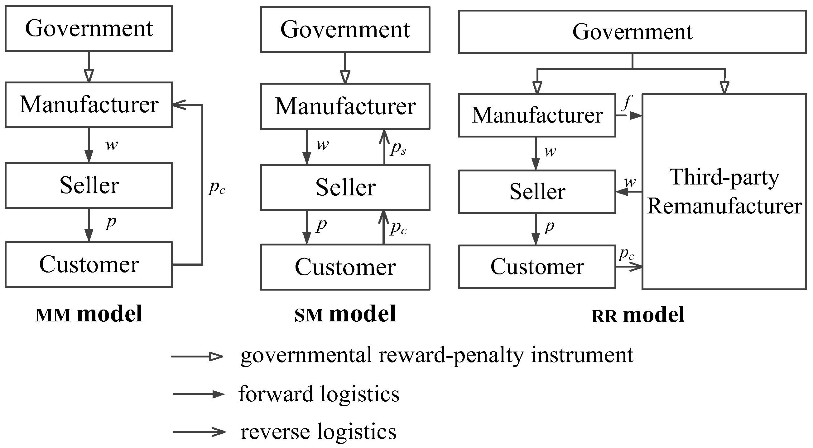
We approach three remanufacturing models in view of distinct collection and remanufacturing undertakers, which are also shown in Figure 1.

(1)

Manufacturer-collection and manufacturer-remanufacturing model (MM model): The manufacturer collects waste products from customers for reutilization. The MM model is a prevailing format of remanufacturing applied by enterprises, such as Hewlett-Packard (HP) and Kodak for instance, in developed regions.

(2)

Seller-collection and manufacturer-remanufacturing model (SM model): The seller bears up waste take-back duties and delivers the EOL products to the manufacturer for remanufacturing. Some Chinese remanufacturing firms adopt such a mode, and part of the home appliance collection business of the Suning Corporation can be referred to as a typical example.

(3)

Remanufacturer-collection and remanufacturer-remanufacturing model (RR model): A third-party remanufacturing mode prevalently implemented in the United States (USA), where the remanufacturer takes the place of the original manufacturer, and engages in product collection and reproduction. Firms such as Caterpillar and Napa, authorized by some machinery companies with specific brands, are currently implementing remanufacturing operations in response to market demand.

3.2. Variables and Parameters Notations

For all of the collection and remanufacturing models mentioned above, mathematical symbols of relevant variables and parameters are given in

Table 1. Symbols and definitions.

Symbols	Definitions
w	Unit wholesale price of new and remanufactured products.
p	Unit sales price of new and remanufactured products.
η	Remanufacturing rate of waste products, $\eta \in [0,1]$.
f	Licensing fee charged by the original manufacturer from third-party remanufacturer for authorization remanufacturing.
i	i = M, S, R, and T represent the manufacturer, the seller, the remanufacturer, and the whole CLSC system, respectively.
j	j = MM, SM, and RR represent the MM model, the SM model, and the RR model, respectively.
cn	Unit production cost of new products.
cr	Unit production cost of remanufactured products.
$\Delta$	Unit cost saving when remanufacturing substitutes regular production, which consumes raw materials, $\Delta =c_n-c_r>0$.
pS	Unit collection cost of waste products from the seller.
pC	Unit collection cost of waste products from customers.
Q	Market demand of the product, $Q=D(p)=a-bp+\epsilon$.
a	Market capacity of the product, $a>0$.
b	Price elasticity coefficient, $b>0$.
ε	Exogenous uncertainties of market demand, $\epsilon \in (0,{\sigma }^2)$.
QR	Remanufacturing quantity of waste products, $Q_R=\eta Q$.
I	Investment in the take-back efforts of waste products, which includes collection system establishment and advertisement expenditures, $I=k_i{\eta }^2$.
ki	Distinct effort costs distributed among the manufacturer, the remanufacturer, and the seller.
L	Governmental rewards or punishments for remanufacturing, $L=\theta (\eta -{\eta }_0)Q$.
${\eta }_0$	Elementary remanufacturing ratio set by the government, ${\eta }_0\in [0,1]$.
$\theta$	Unit amount of reward–penalty allocated by the government, $\theta >0$.
$\mu$	Sharing coefficient of rewards or punishments under the RR model, $\mu \in [0,1]$
${\pi }_i^j$	Profits of member i in the supply chain under collection and remanufacturing model j.

.

Supplementary explanations of the above variables and parameters are provided as follows.

(1)

w, p, η, and f are the decision variables of the CLSC members, while the remaining mathematical symbols are pertinent parameters in model formulations.

(2)

The unit collection costs of p_S and p_C, and the unit cost saving of $\Delta$, satisfy $0\le p_C<p_S\le \Delta$.

(3)

The investment in the take-back efforts of waste products I constitutes a part of the total collection cost $C(\eta )$. Defining that $I=k_i{\eta }^2$ [1], where k_i, and i = M, S, and R, which indicate the respective effort costs distributed among the manufacturer, the seller, and the remanufacturer.

(4)

Rewards or punishments under the RR model are linearly divided between the manufacturer and the remanufacturer by a sharing coefficient $\mu$, $\mu \in [0,1]$. Therefore, $\mu L$ and $(1-\mu )L$ are respective awards/fines imposed on the original manufacturer and the third-party remanufacturer.

3.3. Model Assumptions

To facilitate problem formulation, the concerning remanufacturing CLSC is constructed under the following assumptions after referring to previous studies and practical examples.

Assumption 1.

The supply chain faces a completely open market, where channel members regarding a manufacturer, a seller, and a third-party remanufacturer share symmetric information, for the sake of risk aversion and the operational enhancement of the supply chain [33].

Assumption 2.

All stakeholders involving the original manufacturer, the seller, and the remanufacturer are assumed to be economically rational, pursuing their own profit maximum [34,35].

Assumption 3.

Remanufactured products are highly homogeneous, with brand new ones in commodity ranges and quality performance, hence share the same wholesale and sales price [36,37].

By sorting, testing, dismantling, repairing, disassembling, reusing, and refurbishing with advanced techniques, the quality and performance of remanufactured commodities are either similar to or even more superior than new products. Therefore, the remanufactured products in some respects are assumed to be homogeneous to the new commodities.

Assumption 4.

Both newly and secondary-made products are traded in the same market, the whole quantity of which equals consumption demand Q [25,37].

Assumption 5.

In order to focus analyses on the strategy selections of remanufacturing implementations, we assume that all of the recycled waste products are qualified enough to be put into reproduction after going through comprehensive detection and evaluation [1].

However, in practical operations, recycled materials should be re-examined by the manufacturer or the remanufacturer to further testify their qualities. A small part of them that are unqualified for reproduction will be disposed and then abandoned.

Assumption 6.

Decision-making processes among members are in line with the principles of a Stackelberg game [35,38]. The manufacturer acts as the leader, who guides the seller and remanufacturer to take actions.

Assumption 7.

A single-stage game among supply chain members is discussed without regard for product life cycle, which would requires dynamic game analyses. We consider that the single period of games between the CLSC and the government is profound enough to illustrate the problem and acquire sufficient conclusions [39,40].

4. Strategy Selections under Distinct Remanufacturing Models

In this section, cases of manufacturer-remanufacturing and remanufacturer-remanufacturing are analyzed, with decision-making processes and games among pertinent stakeholders illuminated.

4.1. Manufacturer-Remanufacturing without Authorization

In the absence of authorization remanufacturing, the manufacturer implements waste product reproduction, while collection activities could be maintained by itself or retailer-outsourcing. Thereby, two collection and remanufacturing models showing as MM and SM are established.

4.1.1. Manufacturer-Collection and Manufacturer-Remanufacturing (MM Model)

In the mode of manufacturer collection and remanufacturing, which is noted as the MM model, the manufacturer and the seller make decisions in pursuit of their own profit maximization [34,35,38]. The manufacturer acts as the leader, who determines the wholesale price w and remanufacturing rate η first; then, the retailer follows to decide the sales price, p. The profit functions of the channel members and the whole system ${\pi }_M^{MM}$, ${\pi }_S^{MM}$, ${\pi }_T^{MM}$ are identified as:

$$\begin{array}{l}{\pi }_M^{MM}=\left(w-c_n\right)\left(Q-Q_R\right)+\left(w-c_r\right)Q_R+\theta \left(\eta -{\eta }_0\right)Q-C\left(\eta \right)\\ \hspace{1em}=\left[w-c_n-\theta {\eta }_0+\left(\Delta +\theta -p_C\right)\eta \right]\left(a-bp\right)-k_M{\eta }^2\end{array},$$

(1)

$${\pi }_S^{MM}=\left(p-w\right)Q=\left(p-w\right)\left(a-bp\right),$$

(2)

$${\pi }_T^{MM}={\pi }_M^{MM}+{\pi }_S^{MM}=\left[p-c_n-\theta {\eta }_0+\left(\Delta +\theta -p_C\right)\eta \right]\left(a-bp\right)-k_M{\eta }^2.$$

(3)

4.1.2. Seller-Collection and Manufacturer-Remanufacturing (SM Model)

When the manufacturer remanufactures waste products after outsourcing collection to the retailer in the SM model, channel members make decisions in the same sequence as in the MM model. The seller makes preferential p and collection rate $\eta$ decisions after recognizing the manufacturer’s favorable w according to market demand. Profits of ${\pi }_M^{SM}$, ${\pi }_S^{SM}$, and ${\pi }_T^{SM}$ can be obtained as follows:

$$\begin{array}{l}{\pi }_M^{SM}=\left(w-c_n\right)\left(Q-Q_R\right)+\left(w-c_r\right)Q_R+\theta \left(\eta -{\eta }_0\right)Q-p_S{Q}_R\\ \hspace{1em}=\left[w-c_n-\theta {\eta }_0+\left(\Delta +\theta -p_S\right)\eta \right]\left(a-bp\right)\end{array},$$

(4)

$${\pi }_S^{SM}=\left(p-w\right)Q+p_S{Q}_R-C\left(\eta \right)=\left[p-w+\left(p_S-p_C\right)\eta \right]\left(a-bp\right)-k_S{\eta }^2,$$

(5)

$${\pi }_T^{SM}={\pi }_M^{SM}+{\pi }_S^{SM}=\left[p-c_n-\theta {\eta }_0+\left(\Delta +\theta -p_C\right)\eta \right]\left(a-bp\right)-k_S{\eta }^2.$$

(6)

4.1.3. Comparisons of MM Model and SM Model

According to the aforementioned Stackelberg game between the manufacturer and the seller, we have equilibrium solutions of wholesale price, sales price, actual remanufacturing rate, market demand, remanufacturing quantity, and channel profits, as listed in

Table 2. Equilibrium solutions of the manufacturer-collection and manufacturer-remanufacturing model (MM) model and seller-collection and manufacturer-remanufacturing (SM) model.

	MM Model	SM Model
$w^{\ast }$	$\frac{4k_{M}A-ab{(\Delta +\theta -p_C)}^2}{b[8k_M-b{(\Delta +\theta -p_C)}^2]}$	$\frac{A\left[4k_S-b{(p_S-p_C)}^2\right]-2ab(p_S-p_C)(\Delta +\theta -p_S)}{2b\left[4k_S-b(p_S-p_C)(\Delta +\theta -p_C)\right]}$
$p^{\ast }$	$\frac{2k_{M}A+a\left[4k_M-b{(\Delta +\theta -p_C)}^2\right]}{b\left[8k_M-b{(\Delta +\theta -p_C)}^2\right]}$	$\frac{k_S(2a+A)-ab(p_S-p_C)(\Delta +\theta -p_C)}{b\left[4k_S-b(p_S-p_C)(\Delta +\theta -p_C)\right]}$
${\eta }^{\ast }$	$\frac{B(\Delta +\theta -p_C)}{8k_M-b{(\Delta +\theta -p_C)}^2}$	$\frac{B(p_S-p_C)}{2\left[4k_S-b(p_S-p_C)(\Delta +\theta -p_C)\right]}$
${\mathrm{Q}}^{\ast }$	$\frac{2k_{M}B}{8k_M-b{(\Delta +\theta -p_C)}^2}$	$\frac{k_{S}B}{4k_S-b(p_S-p_C)(\Delta +\theta -p_C)}$
${\mathrm{Q}}_R^{\ast }$	$\frac{2k_M{B}^2(\Delta +\theta -p_C)}{{\left[8k_M-b{(\Delta +\theta -p_C)}^2\right]}^2}$	$\frac{k_S{B}^2(p_S-p_C)}{2{\left[4k_S-b(p_S-p_C)(\Delta +\theta -p_C)\right]}^2}$
${\pi }_S^{j^{\ast }}$	$\frac{4k_M^2{B}^2}{b{\left[8k_M-b{(\Delta +\theta -p_C)}^2\right]}^2}$	$\frac{k_S{B}^2\left[4k_S-b{(p_S-p_C)}^2\right]}{4b{\left[4k_S-b(p_S-p_C)(\Delta +\theta -p_C)\right]}^2}$
${\pi }_M^{j^{\ast }}$	$\frac{k_M{B}^2}{b\left[8k_M-b{(\Delta +\theta -p_C)}^2\right]}$	$\frac{k_S{B}^2}{2b\left[4k_S-b(p_S-p_C)(\Delta +\theta -p_C)\right]}$
${\pi }_T^{j^{\ast }}$	$\frac{k_M{B}^2\left[12k_M-b{(\Delta +\theta -p_C)}^2\right]}{b{\left[8k_M-b{(\Delta +\theta -p_C)}^2\right]}^2}$	$\frac{k_S{B}^2\left[12k_S-b(p_S-p_C)(2\Delta +2\theta +p_S-3p_C)\right]}{4b{\left[4k_S-b(p_S-p_C)(\Delta +\theta -p_C)\right]}^2}$

¹ $A=a+b{c}_n+b\theta {\eta }_0$, $B=a-b{c}_n-b\theta {\eta }_0$.

.

Proof. 

All proofs are provided in Appendix A.

In order to give an intuitive vision of the mathematical results above, a typical numerical analysis is presented to investigate the relations between variables and parameters under both MM and SM models. In accordance with the problem illustrations and model assumptions in Section 3, parameter assignments should meet certain prerequisites that conform to practical operations. To illustrate, $\Delta =c_n-c_r>0$, $0\le p_C<p_S\le \Delta$ should be satisfied, which can be justified by the realities that remanufactured products are less costly than new ones, and the take-back efforts of waste products from the seller naturally cost more than directly collecting the products from customers. $p_C<p_S\le \Delta$ indicate that the unit cost for the collection of waste products should be limited by the unit cost-saving of production. The respective effort costs distributed among the manufacturer, the seller, and the remanufacturer, k_i, i = M, S, R, should meet the common knowledge of $k_M>k_R>k_S>0$, which can be reasonably proved in the following Proposition 3. For the remanufacturing sector of household appliances, electronic instrumentation, vehicles, and their components, we consider that the market capacity of a is relatively large, and the price elasticity coefficient b is comparatively small. Relevant parameters are set as $c_n=30$, $c_r=20$, $\Delta =c_n-c_r=10$, $p_S=8$, $p_C=4$, $a=300$, $b=0.2$, $k_M=3000$, $k_R=1200$, $k_S=500$, and $\eta \in \left[0,1\right]$. Various elementary remanufacturing ratios are allocated to probe into the relations between the actual remanufacturing rate, the unit amount of reward–penalty, and profits of the CLSC members: all of the analytical processes and results are essential for firms to make sensible strategies. In practice, the unit amount of reward–penalty $\theta$ directly measures governmental fiscal power in managing remanufacturing initiatives, and the elementary remanufacturing ratio ${\eta }_0$ signifies the regulatory requirements that should be met, essentially. In general, the fiscal instruments and the elementary remanufacturing ratio have the respective tendencies of descent and ascent in a company according to the expansion of the remanufacturing industry.

(1) Relations of actual remanufacturing rate, elementary remanufacturing ratio, and unit amount of reward–penalty under the MM model and SM model.

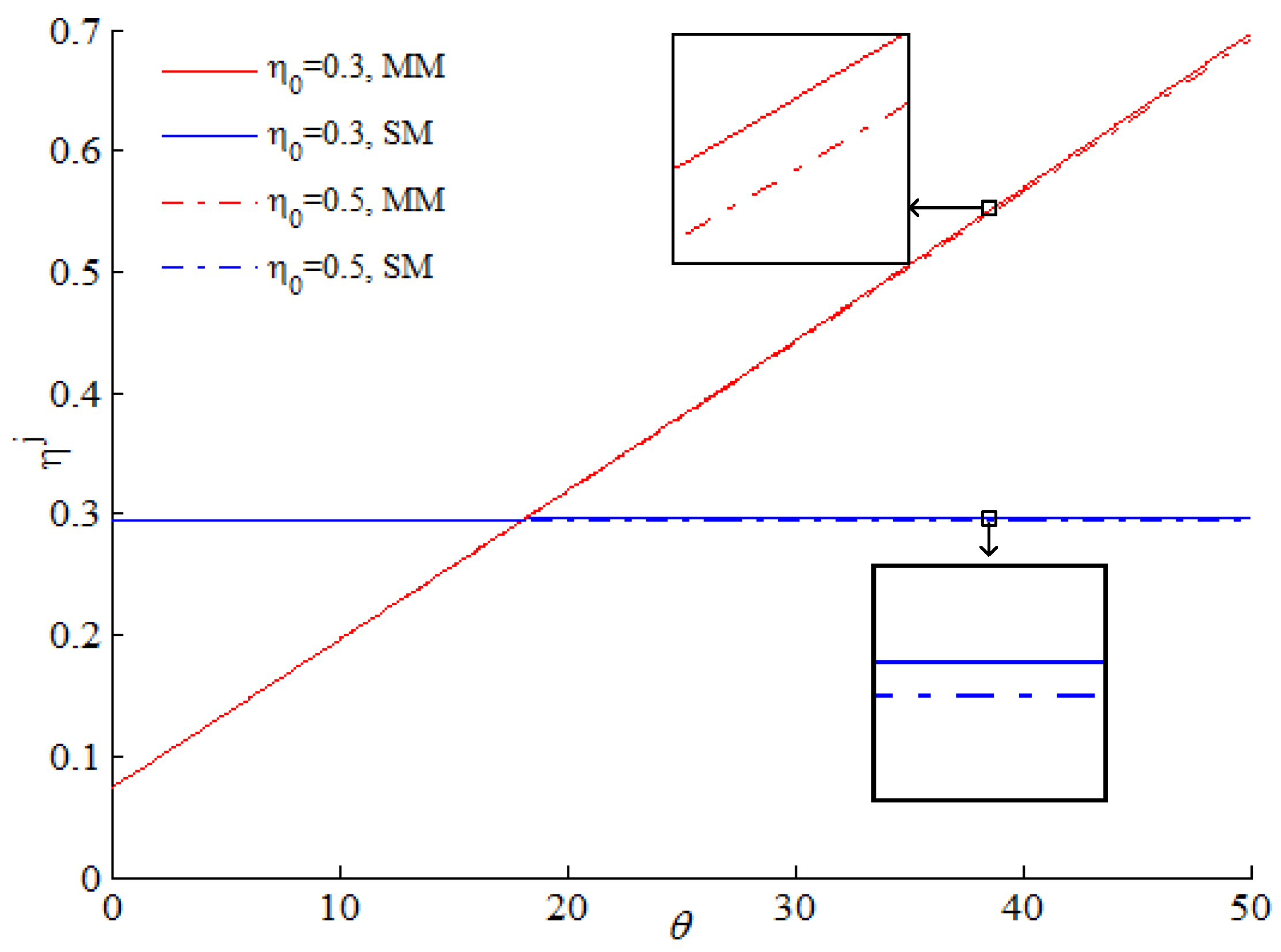
Suppose that the elementary remanufacturing ratio ${\eta }_0$ stays at either 0.3 or 0.5, relations of η, ${\eta }_0$, and $\theta$ are depicted in Figure 2. As we can capture, the actual remanufacturing rate η decreases with the increase of elementary remanufacturing ratio ${\eta }_0$, but is linearly related to $\theta$ in both the MM and SM models. In particular, ${\eta }^{MM}$ is more sensitive to $\theta$ in comparison with ${\eta }^{SM}$. It can be explained by the manufacturer’s stronger desire to attain awards or avoid punishments when facing reward–penalty measures directly in the MM model.

Observation 1.

• To attain a higher remanufacturing rate in reality, it is advisable for the government to raise the unit amount of reward–penalty and cut the elementary remanufacturing ratio. Through such endeavors, an advanced resource circulation system is excepting to be established with the help of the elevated actual remanufacturing rate of the manufacturers.
• When a government’s reward–penalty measures vary, the actual remanufacturing rate in the MM model is more responsive than that in the SM model. Such a result is partly due to the more direct and consequential impacts of rewards or penalties that the government imposes on the manufacturer in the MM model.

(2) Relations among the manufacturer’s profits, the elementary remanufacturing ratio, and the unit amount of reward–penalty under the MM model and SM models.

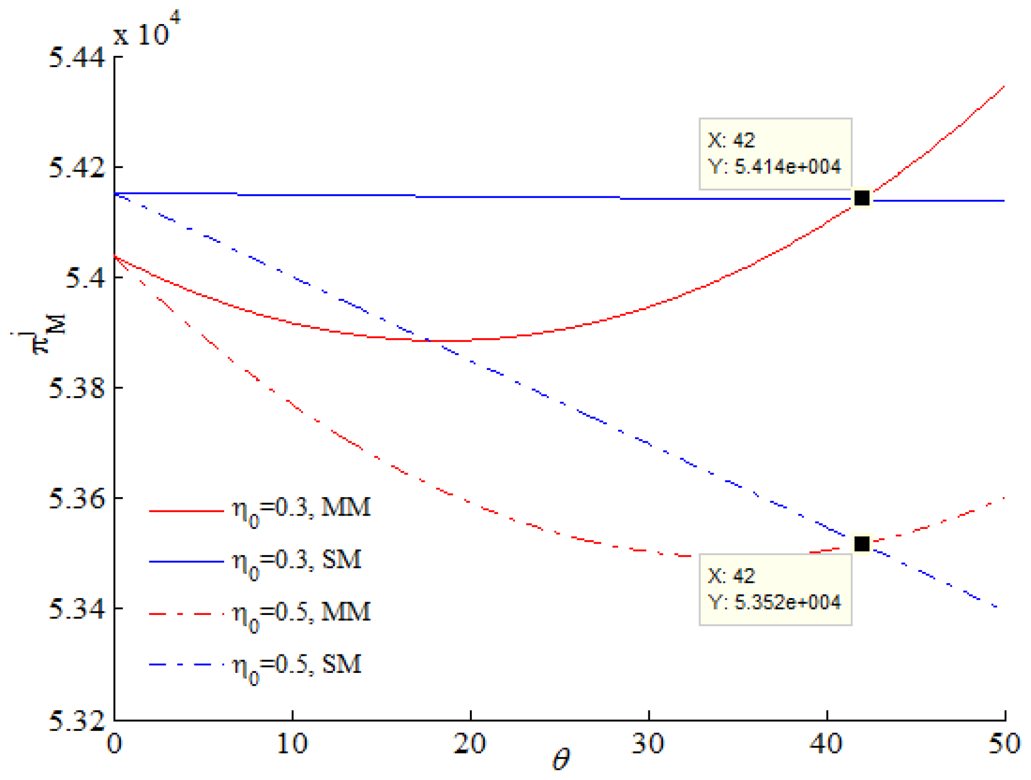
From Figure 3, we notice that the profits of the manufacturer vary contrary to the change of the elementary remanufacturing ratio ${\eta }_0$. ${\pi }_M^{MM}$ is convexly related to $\theta$; it descends first and then increases, while ${\pi }_M^{SM}$ and $\theta$ are negatively interrelated. Specifically, ${\pi }_M^{SM}>{\pi }_M^{MM}$ when $\theta <42$ can be spotted; the rational manufacturer will chose the SM model to achieve maximized profit, while the alternative MM model would be preferred when $\theta >42$.

(3) Relations among the seller’s profits, the elementary remanufacturing ratio, and the unit amount of reward–penalty under the MM model and SM model.

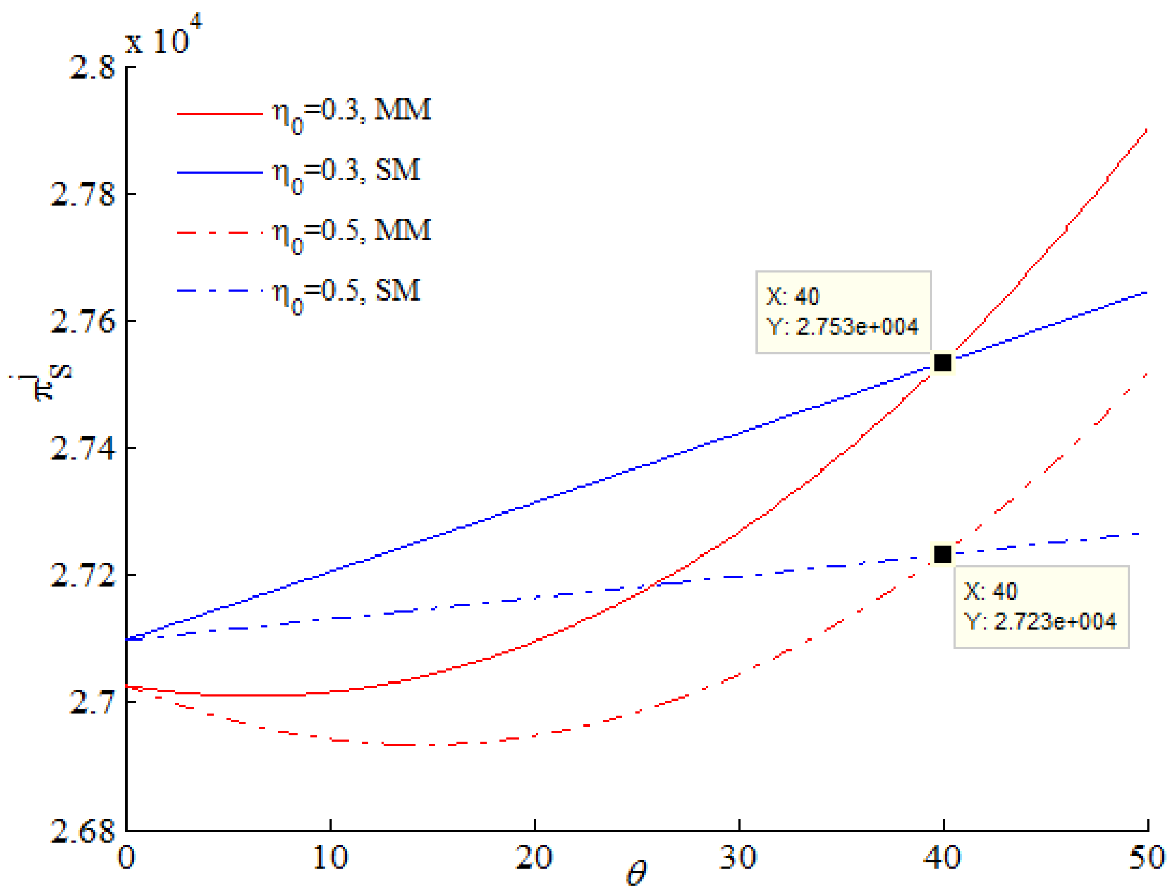
From Figure 4, relations between the seller’s profits and ${\eta }_0$ appear to have the same tendencies as those in Figure 3. Profits of the seller are under the influences of the fiscal instrument: ${\pi }_S^{SM}$ in Figure 4 is positively correlated with $\theta$ expressly. Besides, Figure 4 presents a typical case in which ${\pi }_S^{SM}>{\pi }_S^{MM}$ when $\theta <40$, and the seller will turn to the SM model reasonably. While $\theta >40$ is encountered, on the contrary, predictable results of ${\pi }_S^{SM}<{\pi }_S^{MM}$ will guide the seller to choose the MM model.

Observation 2.

• The increase of the elementary remanufacturing ratio allocated by the government counts against the improvement of the supply chain members’ benefits. As for the relations between the profits of enterprises and the unit amount of reward–penalty imposed by the government, convex correlations can be captured in the MM model. However, in the SM model, strict fiscal measures facilitate the seller in profiting, but are detrimental to the manufacturer.
• When the manufacturer undertakes remanufacturing initiatives, and either itself or the seller conducts waste products collection: (1) If the unit amount of reward–penalty stays within a specified threshold, the profits of the manufacturer, the seller, and the whole channel under the SM model keep an overwhelming advantage over those in the context of the MM model. (2) On the contrary, enhanced reward–penalty measures that stipulate higher rewards and punishments (a greater value of $\theta$) will guide the seller to turn to the MM model.
• Rational manufacturers and sellers in the CLSC system would predictably make sensible model selections between the MM and SM after identifying the strength of the fiscal instruments. In general, the MM model is competitive for both supply chain members when strict reward–penalty measures are adopted.

4.2. Remanufacturer-Remanufacturing Mode with Authorization

In the presence of authorization remanufacturing, the third-party remanufacturer bears up an exhaustive procedure of waste product recycling and reproduction. In a remanufacturer-collection and remanufacturer-remanufacturing mode (noting as the RR model), legislative rewards and punishments are allocated to the manufacturer of $\mu L$, while the remaining $(1-\mu )L$ applies to the remanufacturer.

Channel members in the RR model make decisions in a sequence as ‘manufacturer—remanufacturer—seller’. The manufacturer sets the sales price w and licensing fee f based on its production plan, and then the remanufacturer distributes the remanufacturing rate of the EOL products η. As a matter of course, the remanufacturer determines a certain amount for the collection and remanufacturing of the waste products. The seller takes the last step for the determination of the sales price. The profit functions of the three stakeholders are given as follows:

$$\begin{array}{l}{\pi }_M^{RR}=\left(w-c_n\right)\left(Q-Q_R\right)+\mu L+f{Q}_R\\ \hspace{1em}=\left[w-c_n-\mu \theta {\eta }_0-\left(w-c_n-\mu \theta -f\right)\eta \right]\left(a-bp\right)\end{array},$$

(7)

$$\begin{array}{l}{\pi }_R^{RR}=\left(w-c_r-f\right)Q_R+\left(1-\mu \right)L-C\left(\eta \right)\\ \hspace{1em}=\left\{\left[w-c_r-f-p_C+\left(1-\mu \right)\theta \right]\eta -\left(1-\mu \right)\theta {\eta }_0\right\}\left(a-bp\right)-k_R{\eta }^2\end{array},$$

(8)

$${\pi }_S^{RR}=\left(p-w\right)Q=\left(p-w\right)\left(a-bp\right),$$

(9)

$${\pi }_T^{RR}={\pi }_M^{RR}+{\pi }_R^{RR}+{\pi }_S^{RR}=\left[p-c_n-\theta {\eta }_0+\left(\Delta +\theta -p_C\right)\eta \right]\left(a-bp\right)-k_R{\eta }^2.$$

(10)

Backward induction [41,42] is applied in calculating, which solves decision variables in the order of ‘seller—remanufacturer—manufacturer’. To determine the sales price, we have the following Equation (11) derived from the first order linear condition of Equation (9) to p:

$$p=\frac{a+bw}{2b}.$$

(11)

Plug Equation (11) into Equation (8), and we have the optimal first order condition of η showing as:

$$\eta =\frac{a-bw}{4k_R}\left[w+\left(1-\mu \right)\theta -c_r-f-p_C\right].$$

(12)

Equations (11) and (12) are simultaneously put into Equation (7), to obtain first order conditions of f and w under the prerequisite that the negative definite of the Hessian matrix is satisfied:

$$f^{\ast }=\frac{8k_R\left(a+b{c}_n+\mu b\theta {\eta }_0\right)-ab{\left(\Delta +\theta -p_C\right)}^2}{b\left[16k_R-b{\left(\Delta +\theta -p_C\right)}^2\right]}-\frac{c_n+c_r+p_C+2\mu \theta -\theta }{2},$$

(13)

$$w^{R{R}^{\ast }}=\frac{8k_R\left(a+b{c}_n+\mu b\theta {\eta }_0\right)-ab{\left(\Delta +\theta -p_C\right)}^2}{b\left[16k_R-b{\left(\Delta +\theta -p_C\right)}^2\right]}.$$

(14)

Put Equations (13) and (14) into Equations (11) and (12), and we have:

$$p^{R{R}^{\ast }}=\frac{4k_R\left(3a+b{c}_n+\mu b\theta {\eta }_0\right)-ab{\left(\Delta +\theta -p_C\right)}^2}{b\left[16k_R-b{\left(\Delta +\theta -p_C\right)}^2\right]},$$

(15)

$${\eta }^{R{R}^{\ast }}=\frac{\left(a-b{c}_n-\mu b\theta {\eta }_0\right)\left(\Delta +\theta -p_C\right)}{16k_R-b{\left(\Delta +\theta -p_C\right)}^2}.$$

(16)

Further calculations of market demand and remanufacturing quantity are expressed as:

$$Q^{R{R}^{\ast }}=a-b{p}^{R{R}^{\ast }}=\frac{4k_R\left(a-b{c}_n-\mu b\theta {\eta }_0\right)}{16k_R-b{\left(\Delta +\theta -p_C\right)}^2},$$

(17)

$$Q_R^{R{R}^{\ast }}={\eta }^{R{R}^{\ast }}{Q}^{R{R}^{\ast }}=\frac{4k_R{\left(a-b{c}_n-\mu b\theta {\eta }_0\right)}^2\left(\Delta +\theta -p_C\right)}{{\left[16k_R-b{\left(\Delta +\theta -p_C\right)}^2\right]}^2}.$$

(18)

Now we can substitute optimal solutions of $f^{\ast }$, $w^{R{R}^{\ast }}$, $p^{R{R}^{\ast }}$, ${\eta }^{R{R}^{\ast }}$, $Q^{R{R}^{\ast }}$, and $Q_R^{R{R}^{\ast }}$ into profit functions of Equations (7)–(10), so we obtain:

$${\pi }_M^{R{R}^{\ast }}=\frac{2k_R{\left(a-b{c}_n-\mu b\theta {\eta }_0\right)}^2}{b\left[16k_R-b{\left(\Delta +\theta -p_C\right)}^2\right]},$$

(19)

$${\pi }_R^{R{R}^{\ast }}=\frac{k_R{\left(a-b{c}_n-\mu b\theta {\eta }_0\right)}^2{\left(\Delta +\theta -p_C\right)}^2}{{\left[16k_R-b{\left(\Delta +\theta -p_C\right)}^2\right]}^2}-\frac{4k_R\theta {\eta }_0\left(1-\mu \right)\left(a-b{c}_n-\mu b\theta {\eta }_0\right)}{16k_R-b{\left(\Delta +\theta -p_C\right)}^2},$$

(20)

$${\pi }_S^{R{R}^{\ast }}=\frac{16k_R^2{\left(a-b{c}_n-\mu b\theta {\eta }_0\right)}^2}{b{\left[16k_R-b{\left(\Delta +\theta -p_C\right)}^2\right]}^2},$$

(21)

$$\begin{array}{ll}{\pi }_T^{R{R}^{\ast }}=& \frac{16k_R^2\left(a-b{c}_n-\mu b\theta {\eta }_0\right)\left(3a+\mu b\theta {\eta }_0-3b{c}_n-4b\theta {\eta }_0\right)}{b{\left[16k_R-b{\left(\Delta +\theta -p_C\right)}^2\right]}^2}\\ & -\frac{k_{R}b{\left(\Delta +\theta -p_C\right)}^2\left(a-b{c}_n-\mu b\theta {\eta }_0\right)\left(a+3\mu b\theta {\eta }_0-b{c}_n-4b\theta {\eta }_0\right)}{b{\left[16k_R-b{\left(\Delta +\theta -p_C\right)}^2\right]}^2}\end{array}.$$

(22)

In the light of the above equilibrium solutions of licensing fee $f^{\ast }$, actual remanufacturing rate ${\eta }^{R{R}^{\ast }}$, profits of the manufacturer ${\pi }_M^{R{R}^{\ast }}$, and that of the remanufacturer ${\pi }_R^{R{R}^{\ast }}$, governmental reward–penalty amount $\theta$, reward and punishment sharing factor μ, and elementary remanufacturing ratio ${\eta }_0$, related interrelations of mentioned variables are analyzed, resulting in the following propositions.

Proposition 1.

The optimal licensing fee $f^{\ast }$ and actual remanufacturing rate ${\eta }^{R{R}^{\ast }}$ in the RR model show respective positive and negative variations to the elementary remanufacturing rate ${\eta }_0$, and are negatively influenced by reward–penalty sharing factor μ. Therefore, a greater ${\eta }_0$ value will contribute to a higher $f^{\ast }$ value, but impedes the increase of ${\eta }^{R{R}^{\ast }}$. On the other hand, a slighter μ assists in generating significant $f^{\ast }$ and ${\eta }^{R{R}^{\ast }}$ values concurrently, both of which will benefit the manufacturer as well as the whole remanufacturing operation.

Proposition 2.

The profit of the manufacturer ${\pi }_M^{R{R}^{\ast }}$ and the remanufacturer ${\pi }_R^{R{R}^{\ast }}$ are negatively related with variations of ${\eta }_0$ and μ, and have convex correlations with the unit amount of reward–penalty $\theta$. Such relations indicate that moderate allocations of an elementary remanufacturing ratio and reward–penalty sharing factor, as proactive adoptions of reward and punishment measures, would contribute to enhanced profits of both the manufacturer and remanufacturer in the RR model.

4.3. Comparisons of the MM Model, SM Model, and RR Model

All solutions of the actual remanufacturing rate achieved above should meet the prerequisite of ${\eta }^{\ast }\in \left[0,1\right]$; therefore, Proposition 3 can be obtained.

Proposition 3.

$$k_M\ge \frac{1}{8}\left(\Delta +\theta -p_C\right)\left[B+b\left(\Delta +\theta -p_C\right)\right],$$

(23)

$$k_S\ge \frac{1}{8}\left(p_S-p_C\right)\left[B+2b\left(\Delta +\theta -p_C\right)\right],$$

(24)

$$k_R\ge \frac{1}{16}\left(\Delta +\theta -p_C\right)\left[\left(a-b{c}_n-\mu b\theta {\eta }_0\right)+b\left(\Delta +\theta -p_C\right)\right],$$

(25)

$k_M>k_R>k_S>0$ derived from above equations is in accordance with common knowledge, as an increased coefficient of investment cost k_i will lead to a burdensome I. This result can be explained by the impacts of distinct geographical distances between the CLSC members and waste products on the recovery investment. The remotest manufacturer suffers a high recycling cost, while the closest, seller, who has easy access to customers, significantly saves such expenditure.

Through comparative analyses of remanufacturing rate ${\eta }^j$, remanufacturing quantity $Q_R^j$, enterprises’ profits ${\pi }_i^j$, fiscal instrument $\theta$, reward–punishment sharing factor μ, and elementary remanufacturing ratio ${\eta }_0$ under three models, the following propositions could be attained.

Proposition 4.

Notwithstanding ${\mathrm{Q}}_R^{MM}$, ${\mathrm{Q}}_R^{RR}$ and ${\mathrm{Q}}_R^{SM}$ present nonlinear positive correlations with $\theta$; all of them are negatively related with ${\eta }_0$. ${\eta }^{MM}$, ${\eta }^{RR}$, and ${\eta }^{SM}$ under three models are showing identical variations to $\theta$ and ${\eta }_0$ with respect positive and negative tendencies. Intuitively, a greater $\theta$ and slighter ${\eta }_0$ will generate considerable remanufactured products and an enhanced remanufacturing rate in reality.

Proposition 5.

Profits of stakeholders ${\pi }_i^j$ in the MM and RR models descend firstly, and then ascend with the increase of $\theta$, showing a convex response to the unit amount of reward–penalty. However, relations between the ${\pi }_i^j$ of the manufacturer and the seller in the SM model and $\theta$ express distinctly as linearly negative and positive correlations, respectively.

In addition to the above propositions, numerical analysis is applied to illuminate further implications. Suppose that $\mu =0.3$, and other parameters stay consistent with those in Section 4.1.3, which are introduced and explained from both theoretical and practical points. Various elementary remanufacturing ratios are set to investigate the correlations between the actual remanufacturing rate and fiscal instruments. Relations between profits and the unit amount of reward–punishment are discussed in the meantime. Through such endeavors, favorable mode selections for the CLSC are excepted to be achieved.

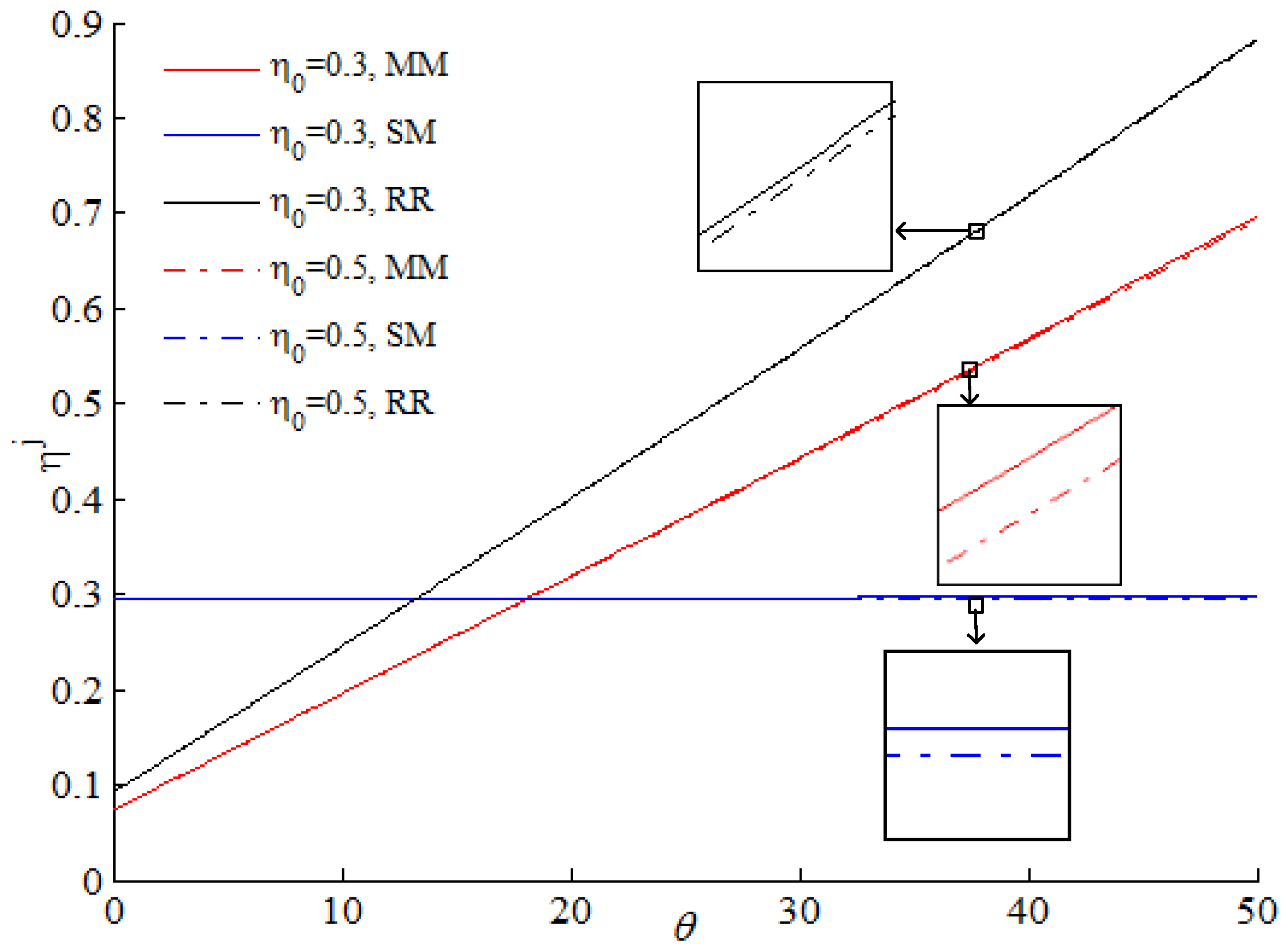
(1) Variation trends of remanufacturing rate ${\eta }^j$ and $\theta$, ${\eta }_0$.

The value of the actual remanufacturing rate validly estimates the renewable availability of resources. Comparing ${\eta }^{MM}$ and ${\eta }^{SM}$ from Figure 5, ${\eta }^{RR}$ is the most responsive to $\theta$, and all ${\eta }^j$ values increase with the decline of ${\eta }_0$ and growth of $\theta$.

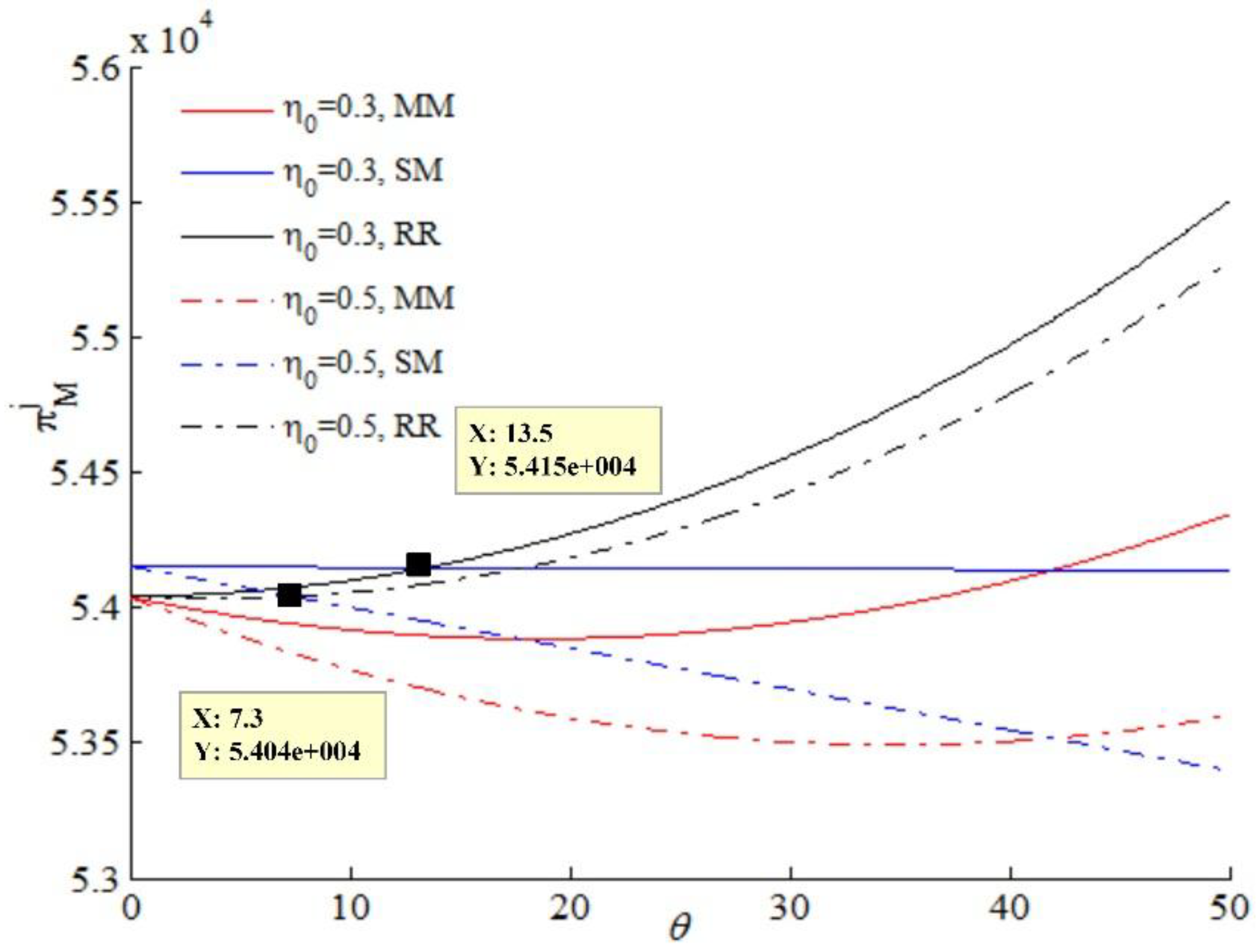
(2) Variation trends of manufacturer’s profits ${\pi }_M^j$ and $\theta$, ${\eta }_0$.

As the core firm in the CLSC system, the manufacturer values its profit as a principal indicator for mode selection. It can be seen from Figure 6 that the manufacturer’s profits under ${\eta }_0=0.3$ remain higher than those under ${\eta }_0=0.5$, which is applicable to all of the models. Besides, $\theta$ excretes convex impacts on ${\pi }_M^j$ under the MM and RR models, and is linearly negative to ${\pi }_M^{SM}$, which imply that the manufacturer will employ appropriate models according to governmental fiscal intensity. When the reward–penalty is underestimated within a certain range—$\theta =13.5$ and $\theta =7.3$ when ${\eta }_0=0.3$ and ${\eta }_0=0.5$, respectively, in Figure 6 for instance—the manufacturer prefers the SM model for product collection and remanufacturing. On the contrary, when $\theta$ happens to be out of the range and stays at a comparatively higher level, the manufacturer will turn to the RR model for more considerable profits.

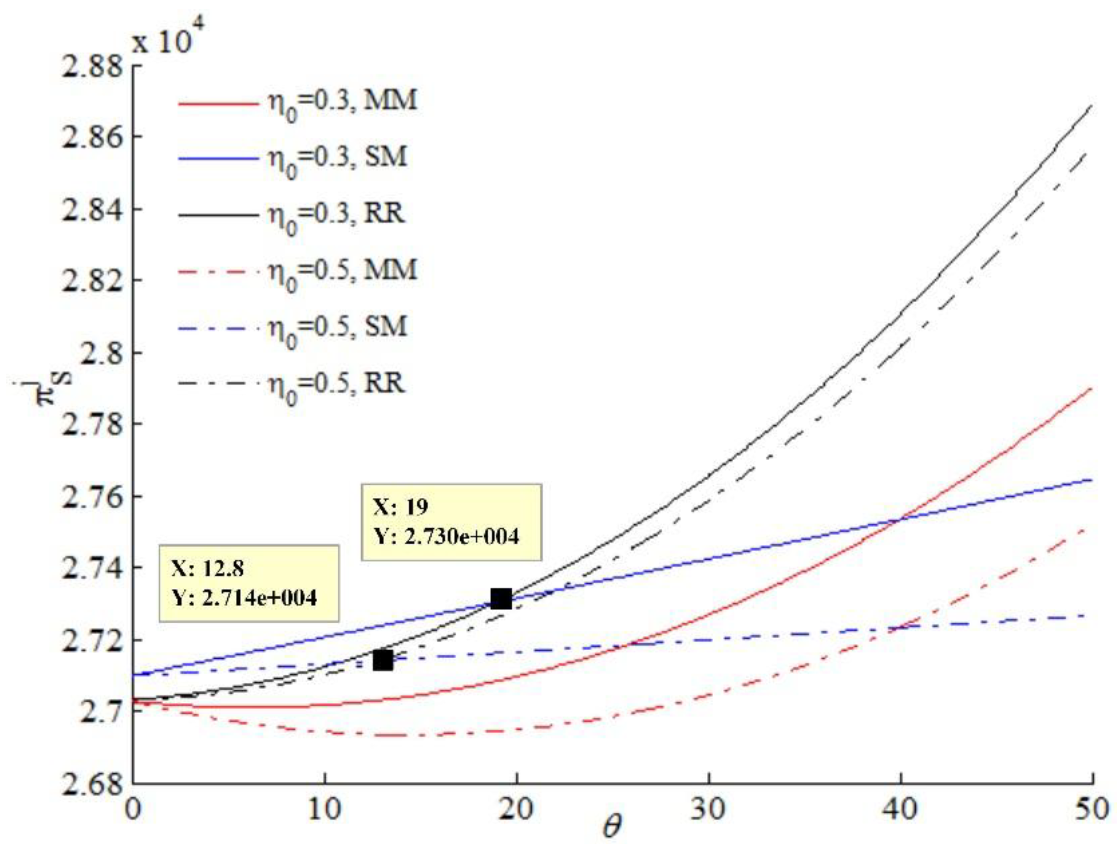
(3) Variation trends of the seller’s profits ${\pi }_S^j$ and $\theta$, ${\eta }_0$.

Profits of the seller have the same variation trends as the diversities among ${\eta }_0$ and $\theta$ in the MM model and the RR model, with those of the manufacturer in Figure 7. ${\pi }_M^{SM}$ in particular is linearly positive to the change of $\theta$. Analogous statements can be concluded that when the unit amount of reward–penalty is under a specific value, as $\theta =19$ and $\theta =12.8$ in the cases of ${\eta }_0=0.3$ and ${\eta }_0=0.5$, respectively, the seller tends to choose the SM model with superior ${\pi }_S^j$, but would otherwise adopt the RR model if $\theta$ reaches a higher value beyond the benchmark.

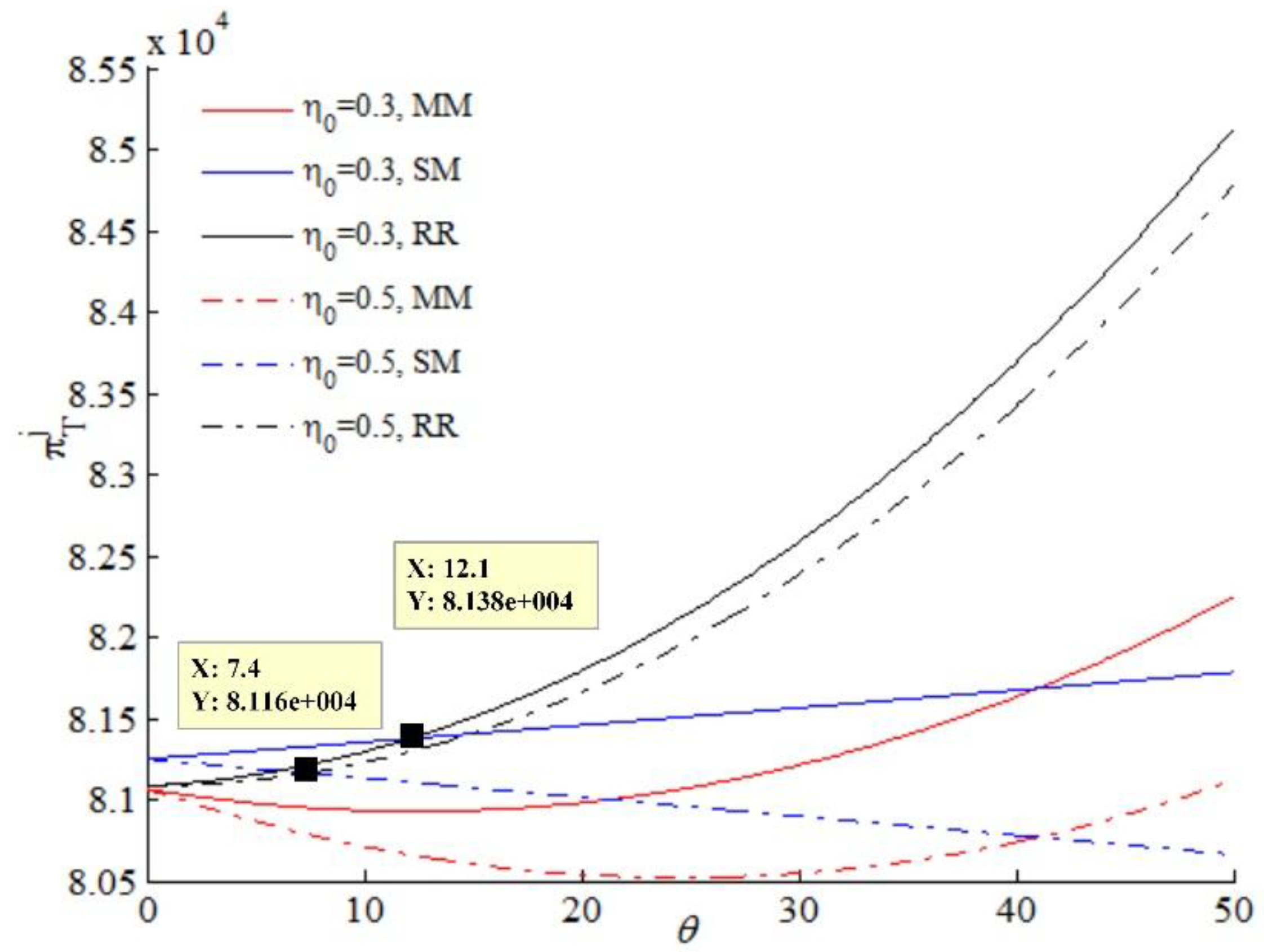
(4) Variation trends of total profits of the CLSC ${\pi }_T^j$ and $\theta$, ${\eta }_0$.

Channel profits in Figure 8 vary opposite to the elementary remanufacturing ratio, and ${\pi }_T^{RR}$ appears to be the least responsive to changes of ${\eta }_0$. Relations between ${\pi }_T^j$ and $\theta$ turn out to be convex in the MM and RR models, while linearly negative correlations occur in the SM model. As such, the optimal profits of the whole system are inevitably influenced by the unit amount of reward–penalty allocated by the government. As the example of $\theta =12.1$ and $\theta =7.4$ when ${\eta }_0=0.3$ and ${\eta }_0=0.5$ in Figure 8 imply, a seller-collection and manufacturer-remanufacturing mode is beneficial for considerable channel profits when the reward–penalty is allocated at a fairly lower level. Yet, supply chain members are most inclined to focus on authorization remanufacturing (the RR model), in order to achieve optimal channel gains as well as integrated profits between the manufacturer and the seller, with a licensing fee charged from the remanufacturer.

Observation 3.

• In all of the collection and remanufacturing models, the actual and elementary remanufacturing ratios are negatively related.
• The actual remanufacturing rates are positively influenced by the unit amount of reward–penalty. Among these, ${\eta }^{RR}$ in the RR model is more responsive to $\theta$ than ${\eta }^{MM}$ and ${\eta }^{SM}$ in the MM and SM models.

Observation 4.

• In the MM and RR models, the profits of the manufacturer, the seller, and the whole system are convexly related with $\theta$ and are negatively influenced by ${\eta }_0$. In general, the profits of all of the stakeholders in the RR model are comparatively more appreciable under certain governmental interventions via fiscal instruments and regulations.
• In the SM model, the unit amount of reward–penalty impacts the profits of the manufacturer and the whole system negatively, but has a positive relationship with the seller’s profits. As the leader in the system, the manufacturer occupies a more essential role in all of the CLSC operations and performances.
• In the SM model, when $\theta$ fails to reach a certain value, the current mode will be the most favored format deployed by the CLSC. On the contrary, when $\theta$ goes out of the threshold, the RR model will take the place of the SM model. In particular, the threshold turns out to be negatively correlated with the elementary remanufacturing rate ${\eta }_0$. Hence, moderate regulation of the government makes the SM model more preferential than its alternatives.

5. Conclusions, Implications, and Directions for Future Research

5.1. Conclusions

Patent protection has been a broad-ranging strategy in maintaining original manufacturers’ benefits by charging licensing fees for brands or authorized technologies, and patented products for remanufacturing are apparently under such exclusive protection. As noted at the outset, the contribution of this paper is to explore optimal strategies for CLSC members in choosing waste product collection and remanufacturing modes under governmental intervention and patent protection. A game-theoretical model is applied to develop two formats of EOL products’ recycling and remanufacturing, which manifest as self-reproduction by the original manufacturer and authorization remanufacturing by the third-party remanufacturer. Manufacturer-collection and manufacturer-remanufacturing (MM), seller-collection and manufacturer-remanufacturing (SM), and remanufacturer-collection and remanufacturer-remanufacturing (RR) models are introduced. Equilibrium quantities, prices, and profits, along with their comparisons under distinct models, are discussed in order to investigate preferential strategies. The main results are summarized as follows.

• higher elementary remanufacturing ratio ${\eta }_0$ allocated by the government is detrimental to the progress of the actual remanufacturing rate in all of the collection and remanufacturing models. On the other hand, strengthened fiscal instruments facilitate the establishment of an advanced resource circulation system by improving the remanufacturing rate in reality (Observation 1, 3; Proposition 4).
• In the MM and SM models without authorization remanufacturing, the actual remanufacturing rate of the manufacturer ${\eta }^{MM}$ is more responsive than ${\eta }^{SM}$ to the unit amount of reward–penalty $\theta$. However, in the presence of third-party remanufacturing under patent protection, ${\eta }^{RR}$ in the RR model turns out to be most responsive to $\theta$ over those in manufacturer-remanufacturing modes (Observation 1, 3).
• In the RR model, the growth of ${\eta }_0$ is beneficial to enhancing the intellectual property rights of the original manufacturer, which leads to an elevated licensing fee f. The reward–penalty sharing coefficient $\mu$, on the contrary, impacts f negatively (Proposition 1).
• In all of the collection and remanufacturing models, the profits of CLSC members are negatively affected by the elementary remanufacturing ratio (Observation 2, 4; Proposition 2).
• (1) In the MM and RR models, the profits of all of the stakeholders, along with the whole channel, are convexly varied with the increase of $\theta$. (2) In the SM model, the profits of the manufacturer and the seller respectively show negative and positive correlations with $\theta$. The profits of the whole CLSC, under both influences of channel members, are negatively impacted by $\theta$, which is consistent with the manufacturer. (Observation 2, 4; Proposition 2, 5).
• (1) When $\theta$ is imposed within a certain threshold, the SM model is more favored than the MM model in the manufacturer-remanufacturing mode. (2) When the third-party remanufacturer participates in product reproduction, the RR model is the most profitable for the CLSC if $\theta$ is allocated at a comparatively higher level. Otherwise, both the manufacturer and the seller prefer the SM model (Observation 2, 4).
• The threshold of $\theta$ in the manufacturer-remanufacturing mode stays constant under the influence of ${\eta }_0$, while it is negatively affected by ${\eta }_0$ when authorization remanufacturing come into notice (Observation 4).
• Distinct effort costs distributed among CLSC members k_i meet the common knowledge of $k_M>k_R>k_S>0$ (Proposition 3).

5.2. Policy and Managerial Implications

The current work is conducted in the realm of the reutilization and remanufacturing of household appliances, electronic instrumentation, mechanical equipment, vehicles, and their components. The strategy selections in the proposed models are applicable to most remanufacturing systems where outsourcing collection and remanufacturing are in parallel with authorization remanufacturing.

The manufacturer, who is possessed with intellectual property rights, primarily refers to the elementary remanufacturing ratio and the unit amount of reward–penalty in selecting models for the collection and remanufacturing of waste products. Governmental policies aiming at raising social welfare, in such contexts, are recommended to enforce resource circulation and environment conservation by incubating an enduring progress for the remanufacturing industry, as specifically setting reasonable and adaptable regulatory and fiscal factors. Implications of policy creation for the government, and strategy selections for the CLSC members, are provided as follows.

From the perspective of the government, reasonable allocations for the elementary remanufacturing ratio and the unit amount of reward–penalty both play a decisive role in the advancement of collection and remanufacturing management.

• It is advisable for the government to raise the reward–penalty amount and cut the mandatory remanufacturing ratio, for the achievement of an elevated remanufacturing rate and increased amount of remanufactured products in reality.

Although a higher elementary remanufacturing ratio could result in increased licensing fees for authorization remanufacturing, it impedes the improvement of the remanufacturing rate in reality, and brings about penalty losses of the CLSC when failing to meet the regulations. Therefore, an excessive elementary remanufacturing rate would discourage the CLSC members other than invigorating their remanufacturing initiatives. The fiscal instrument, on the other hand, is productive in the progress of the collection and remanufacturing system by enhancing CLSC members’ profits and the actual remanufacturing rate.

• Sensible fiscal instruments should be preferred to regulatory measures, especially regarding the management of remanufacturer-remanufacturing model.

In the authorization-remanufacturing mode in particular, the actual remanufacturing rate is the most responsive to the reward–penalty amount, while the profits of the CLSC turn out to be the least responsive to the elementary remanufacturing rate. Therefore, fiscal instruments can be more essential in remanufacturing management.

In general, the fiscal instruments and elementary remanufacturing ratio have respective decreasing and increasing tendencies with the expansion of remanufacturing industry. However, for the emerging industry at its inception, moderate regulation and strict fiscal instruments are recommended for the policy makers.

For firms, prudent and adaptable strategy selections should be made in response to government intervention via regulations and fiscal instruments.

• If the given amount of a reward–penalty set by government appears to be less than a specific value, all of the supply chain members should respond rationally to the SM model. On the contrary, the RR model is the right option for every involved member, in which the third-party remanufacturer assumes both the obligations of remanufacturing and paying licensing fees.
• In particular, the authorization-remanufacturing mode should be embraced, since it is in most cases more profitable than its alternatives. The manufacturer and the seller are able to obtain benefits from the licensing fees charged from the remanufacturer, and reduce collection and reproduction costs with operational efficiency enhanced concurrently.
• The reward–penalty sharing coefficient between the manufacturer and the remanufacturer is suggested to be assigned slightly, which will lead to increased licensing fees and actual remanufacturing rates, as well as profits for both the original manufacturer and the third-party remanufacturer.

5.3. Limitations and Future Research

The game theoretic approach adopted in the current paper jointly addresses the issues of CLSC operation, government regulation, and patent protection that have received continuous attention from both academic and pragmatic fields. Three models of waste product collection and remanufacturing are developed, which are in accordance with practical operation, and can be applied extensively in relevant remanufacturing systems. The results obtained from the game theoretic models are evident and traceable, which are able to provide significant implications from both perspectives of policymakers and enterprises. Therefore, we consider the current approach to be proper and applicable.

Although the current paper, along with its results, has crucial significance from both normative and practical perspectives, the game theoretic approach and model still have several limitations that merit future research.

• It is beyond the scope of our work to analyze CLSC decisions influenced by product differentiation. In practice, newly-made products and remanufactured ones are heterogeneous in customer recognition; this possibility arises when the remanufacturing industry, along with its products in China, is at its inception, and is far from prevailingly accepted. To be specific, the retail price of the remanufactured products is 20–30% cheaper than newly-made commodities, which is partly due to deficient promotion and customer recognition [43,44].
• We do not consider adaptive changes that should be made if relevant stakeholders are risk-preferential; therefore, corresponding risk coefficients will be influential in strategy selections.
• The collection rate of waste products is assumed to be equal to the actual remanufacturing rate. It might be more practical to analyze the actual amount of secondary materials that are re-examined by the manufacturer or the remanufacturer for remanufacturing.
• We consider that all of the stakeholders in the CLSC are completely rational. However, bounded rationality and information asymmetry in reality significantly impact supply chain members regarding strategy adjustments and progresses.
• Multi-period decisions that consider product life cycles are neglected in the current study, which are also worth discussing in future research.

References

- Savaskan, R.C.; Bhattacharya, S.; Van Wassenhove, L.N. Closed-loop supply chain models with product remanufacturing. Manag. Sci. 2004, 50, 239–252. [Google Scholar] [CrossRef]
- Naustdalslid, J. Circular economy in China–the environmental dimension of the harmonious society. Int. J. Sustain. Dev. World Ecol. 2014, 21, 303–313. [Google Scholar] [CrossRef]
- Xu, B.S. Theory and Technology of Equipment Remanufacturing Engineering; National Defense Industry Press: Beijing, China, 2007. [Google Scholar]
- Nie, J.J.; Deng, D.F. Effects of remanufacturing product quality on recovery channel in closed-loop supply chain. Ind. Eng. Manag. 2014, 19, 1–7. [Google Scholar]
- Hatcher, G.D.; Ijomah, W.L.; Windmill, J. Design for remanufacturing in China: A case study of electrical and electronic equipment. J. Remanuf. 2013, 3, 3–19. [Google Scholar] [CrossRef] [Green Version]
- Wongthatsanekorn, W.; Realff, M.; Ammons, J. Multi-time scale Markov decision process approach to strategic network growth of reverse supply chains. Omega 2010, 38, 20–32. [Google Scholar] [CrossRef]
- Toktay, L.B.; Wei, D. Cost allocation in manufacturing-remanufacturing operations. Prod. Oper. Manag. 2011, 20, 841–847. [Google Scholar] [CrossRef]
- Xiong, Z.K.; Wang, K.; Xiong, Y. Research on the closed-loop supply chain that the distributor engages in remanufacturing. J. Manag. Sci. China 2012, 14, 1–9. (In Chinese) [Google Scholar]
- Atasu, A.; Toktay, L.B.; Van Wassenhove, L.N. How collection cost structure drives a manufacturer’s reverse channel choice. Prod. Oper. Manag. 2013, 22, 1089–1102. [Google Scholar] [CrossRef]
- Chen, J.M.; Chang, C.I. Dynamic pricing for new and remanufactured products in a closed-loop supply chain. Int. J. Prod. Econ. 2013, 146, 153–160. [Google Scholar] [CrossRef]
- Xiong, Y.; Zhou, Y.; Li, G.D.; Chan, H.K.; Xiong, Z.K. Don’t forget your supplier when remanufacturing. Eur. J. Oper. Res. 2013, 230, 15–25. [Google Scholar] [CrossRef]
- Xiong, Y.; Zhao, Q.W.; Zhou, Y. Manufacturer-remanufacturing vs supplier-remanufacturing in a closed-loop supply chain. Int. J. Prod. Econ. 2016, 176, 21–28. [Google Scholar] [CrossRef]
- Krumwiedea, D.W.; Sheu, C. A model for reverse logistics entry by third-party providers. Omega 2002, 30, 325–333. [Google Scholar] [CrossRef]
- Chen, L.F.; Wu, G. Applying the principal-agent theory to the study of reverse logistics outsourcing. Math. Pract. Theory 2010, 40, 14–19. (In Chinese) [Google Scholar]
- Wang, N.M.; Sun, Q.L.; Sun, L.Y. Single-item dynamic lot sizing problem with remanufacturing and outsourcing. Oper. Res. Manag. Sci. 2011, 20, 162–168. [Google Scholar]
- Fan, T.J.; Lou, G.X.; Wang, C.L.; Chen, R.Q. Analysis of outsourcing decision-making on used products collection for green manufacturing. J. Manag. Sci. China 2011, 14, 8–15. [Google Scholar]
- Abdulrahman, M.D.; Subramanian, N.; Liu, C.; Shu, C.Q. Viability of remanufacturing practice: A strategic decision making framework for Chinese auto-parts companies. J. Clean. Prod. 2015, 105, 311–323. [Google Scholar] [CrossRef]
- Agrawala, S.; Singh, R.K.; Murtaza, Q. Outsourcing decisions in reverse logistics: Sustainable balanced scorecard and graph theoretic approach. Resour. Conserv. Recycl. 2016, 108, 41–53. [Google Scholar] [CrossRef]
- Yan, W.; Li, H.; Chai, J.; Qian, Z.; Chen, H. Owning or outsourcing? Strategic choice on take-back operations for third-party remanufacturing. Sustainability 2018, 10, 151. [Google Scholar] [CrossRef]
- Xiong, Z.K.; Shen, C.R.; Peng, Z.Q. Closed-loop supply chain coordination research with remanufacturing under patent protection. J. Manag. Sci. China 2011, 14, 76–85. (In Chinese) [Google Scholar]
- Oraiopoulos, N.; Ferguson, M.E.; Toktay, L.B. Relicensing as a secondary market strategy. Manag. Sci. 2012, 58, 1022–1037. [Google Scholar] [CrossRef]
- Xiong, Z.K.; Shen, C.R.; Peng, Z.Q. A remanufacturing strategy for the closed-loop supply chain under patent protection. J. Ind. Eng. Eng. Manag. 2012, 26, 159–165. [Google Scholar]
- He, Y. The Product Design Strategy of the Manufacturer under Patent Protection. Master’s Thesis, Xiamen University, Xiamen, China, 2014. (In Chinese). [Google Scholar]
- Shen, C.R.; Xiong, Z.K.; Meng, W.J. Remanufacturing modes of the closed-loop supply chain under patent protection. J. Syst. Manag. 2015, 24, 123–129. (In Chinese) [Google Scholar]
- Ma, Z.; Qin, Z.; Dai, Y.; Guan, G. To license or not to license remanufacturing business? Sustainability 2018, 10, 347. [Google Scholar] [CrossRef]
- Sheu, J.B. Bargaining framework for competitive green supply chains under governmental financial intervention. Transp. Res. Part E 2011, 47, 573–592. [Google Scholar] [CrossRef]
- Hong, I.H.; Ke, J.S. Determining advanced recycling fees and subsidies in ‘E-scrap’ reverse supply chains. J. Environ. Manag. 2011, 92, 1495–1502. [Google Scholar] [CrossRef] [PubMed]
- Huang, J.; Lei, M.M.; Liang, L.P.; Liu, J. Promoting electric automobiles: Supply chain analysis under a government’s subsidy incentive scheme. IIE Trans. 2013, 45, 826–844. [Google Scholar] [CrossRef]
- Wang, W.B.; Da, Q.L. The decision making of manufacturers for collection and remanufacturing based on premium and penalty mechanism under competition environment. Chin. J. Manag. Sci. 2013, 21, 50–56. (In Chinese) [Google Scholar] [CrossRef]
- Cao, J.; Hu, Q.; Wu, X.B. Incentive mechanism between government and manufacturers based on EPR system. Syst. Eng. Theory Pract. 2013, 33, 610–622. (In Chinese) [Google Scholar]
- Zhang, S.H.; Zhang, J.R.; Chu, Y.P. Pricing and coordination of closed-loop supply chain based on remanufacturing priority. J. Syst. Eng. 2013, 28, 506–512. (In Chinese) [Google Scholar]
- Li, X.R.; Wu, Y.B. Differential price closed-loop supply chain under the government replacement-subsidy. Syst. Eng. Theory Pract. 2015, 35, 1983–1995. (In Chinese) [Google Scholar]
- Pinçe, C.; Ferguson, M.; Toktay, B. Extracting maximum value from consumer returns: Allocating between remarketing and refurbishing for warranty claims. Manuf. Serv. Oper. Manag. 2016, 18, 175–492. [Google Scholar] [CrossRef]
- Cao, J.; Zhang, X.; Zhou, G. Supply chain coordination with revenue-sharing contracts considering carbon emissions and governmental policy making. Environ. Prog. Sustain. Energy 2016, 35, 479–488. [Google Scholar] [CrossRef]
- Tadelis, S. Game Theory: An Introduction; Princeton University Press: Princeton, NJ, USA, 2013. [Google Scholar]
- Orsdemir, A.; Kemahlglu-Ziya, E.; Parlakturk, E.K. Competitive quality choice and remanufacturing. Prod. Oper. Manag. 2014, 28, 48–64. [Google Scholar] [CrossRef]
- Liao, H.; Deng, Q.; Wang, Y. Optimal acquisition and production policy for end-of-life engineering machinery recovering in a joint manufacturing/remanufacturing system under uncertainties in procurement and demand. Sustainability 2017, 9, 338. [Google Scholar] [CrossRef]
- Xie, S.Y. Economic Game Theory; Fudan University Press: Shanghai, China, 2014. [Google Scholar]
- Shu, T.; Wang, Y.; Chen, S.; Wang, S.; Lai, K.; Yang, Y. Decisions on remanufacturing with WTP disparity and recycling competition under government subsidies. Sustainability 2017, 9, 1503. [Google Scholar] [CrossRef]
- Zou, Z.; Wang, J.; Deng, G.; Chen, H. Third-party remanufacturing mode selection: Outsourcing or authorization? Transp. Res. Part E 2016, 87, 1–19. [Google Scholar] [CrossRef]
- Adda, J.; Cooper, R. Dynamic Economic: Quantitative Methods and Applications; MIT Press: Cambridge, MA, USA, 2003. [Google Scholar]
- Kicsinya, R.; Vargaa, Z.; Scarellib, A. Backward induction for a class of closed-loop Stackelberg games. Eur. J. Oper. Res. 2014, 237, 1021–1036. [Google Scholar] [CrossRef]
- Yusop, N.M.; Wahab, D.A.; Saibani, N. Realizing the automotive remanufacturing roadmap in Malaysia: Challenges and the way forward. J. Clean. Prod. 2016, 112, 1910–1919. [Google Scholar] [CrossRef]
- Alqahtani, A.Y.; Gupta, S.M. Warranty as a marketing strategy for remanufactured products. J. Clean. Prod. 2017, 161, 1294–1307. [Google Scholar] [CrossRef]
Figure 1.
Remanufacturing closed-loop supply chain (CLSC) model considering patent protection and government constraints.
Figure 2.
Relations of actual remanufacturing rate and unit amount of reward–penalty under manufacturer-remanufacturing modes.
Figure 3.
Relations between the manufacturer’s profits and the unit amount of reward–penalty under manufacturer-remanufacturing modes.
Figure 4.
Relations of the seller’s profits and unit amount of reward–penalty under manufacturer-remanufacturing modes.
Figure 5.
Relations of actual remanufacturing rate η and the unit amount of reward–penalty θ.
Figure 6.
Relations of the manufacturer’s profits and the unit amount of reward–penalty θ.
Figure 7.
Relations of the seller’s profits and unit amount of reward–penalty θ.
Figure 8.
Relations of channel profits and unit amount of reward–penalty θ.