Article

Effects of Thinning on the Spatial Structure of Larix principis-rupprechtii Plantation

1
College of Soil and Water Conservation, Beijing Forestry University, Beijing 100083, China
2
State Environmental Protection Key Laboratory of Regional Eco-process and Function Assessment, State Key Laboratory of Environmental Criteria and Risk Assessment, Chinese Research Academy of Environmental Sciences, Beijing 100012, China
3
Chinese Academy of Forestry, Institute of Desertification Studies, Beijing 100091, China
*
Author to whom correspondence should be addressed.
Sustainability 2018, 10(4), 1250; https://doi.org/10.3390/su10041250
Submission received: 23 December 2017 / Revised: 15 April 2018 / Accepted: 17 April 2018 / Published: 19 April 2018
(This article belongs to the Special Issue Sustainable Ecology and Forest Management)

Abstract

:
Structure-based forest management is a scientific and easy-to-operate method for sustainable forest management. We analyzed the stand spatial structure of Larix principis-rupprechtii plantation under five reserve densities. The results indicated that with the decrease of densities after thinning, the average mingling degree and uniform angle index had an increasing tendency, but the amplitude was small. Most of the trees were in zero mix, and a few of them were in moderate, strong, and relatively strong mix; the horizontal distribution patterns were uniform or near-uniform random. The distribution of neighborhood comparison and opening degree changed with a fluctuant pattern, but thinning decreased the competitive intensities to some extent. A composite structure index (Ci) was established, based on the relative importance of the above four indicators, to evaluate the overall effect of thinning on stand structure characteristics. The findings showed that Ci increased with the increase of thinning intensity, that is, the stand spatial structure became more complex. This indicated that Ci may be a simple and rapid indicator to evaluate the overall effect of thinning on stand spatial structure within densities after thinning.

1. Introduction

Forest management is a perpetual theme of forestry development, in which the principle is following the law of nature, which, in other words, is abiding by the regular pattern of nature to achieve structural adjustment of the forest, given a certain objective. Forest structure helps us understand the history of forest development, its current condition, and the future development of the ecosystem. This is crucial for analyzing and managing a forest ecosystem [1]. Forest stand structure is one of the important forest ecosystem attributes [2], referring to the spatial distribution of trees, mutual position, diameter, and height differentiation [3]. The spatial structure not only determines the competitive niche and space of trees, but also impacts the stable development and management of stand [4]. The structure of a forest characterized by the diversity of spatial position, species, and dimension, to a greater degree, depends on the spatial relationship of neighborhood trees. Stand spatial structure parameters based on the relationship of neighborhood trees, such as uniform angle index, mingling, and dominance, are widely used both internationally and domestically in the studies of stand spatial structure analysis, competition among trees, calculation of dominance, species diversity measurement, and structure recovery and reconstruction, as well as in optimization adjustment [1]. Thus, how thinning is to be used to optimize the stand spatial structure has been the concern of forest managers [5]. Traditional forest management methods mainly focus on stand age structure, composition structure, and horizontal and vertical structure, using stand age, diameter, height, species composition, density, and distribution patterns of population as indicators. These are significant for the determination of stand quantitative characteristics and population structure, but are not available for uneven-aged and mixed forests [6]. The structure-based management that was recently advocated can promote the active management of stand density through periodic thinning [7,8]. In the last decades, some indictors of stand spatial structure, such as mingling degree, uniform angle index, and neighborhood comparison, were proposed based on traditional methods to evaluate the effect of structure-based forest management and to quantify the uneven-aged and mixed stand spatial structure [9,10,11]. Using these indicators, some studies on spatial structure were conducted, such as the spatial structure change of Fagus longipetiolata forest, optimized spatial model of stand thinning [12], and spatial structure of broad-leaved Korean pine forests [13]. However, current research on forest structure-based management mainly focuses on natural forests, while the research on plantations is rarely reported.
China has the largest plantation area in the world. The FRA (Global Forest Resources Assessment) 2015, published by FAO (Food and Agriculture Organization of the United Nations), showed that the net increases of plantation area and stock volume from 2010 to 2015 in China were 1,542,000 ha and 447 million m3, respectively, and the total was 208,321,000 ha and 1.961 billion m3, respectively [14]. China’s plantation area ranks first in the world [15]. Although the plantation area and stock volume maintain rapid and stable growth, many problems (such as low-quality plantation with only 49.01 m3/hm2 stock volume of forest, unreasonable age group composition, a large ratio of young and middle-aged stand, pest disasters etc.) have resulted in the need for arduous tending [15]. As an important management measure for forest cultivation, thinning can improve forest quality and physical-chemical properties, optimize forest structure, and maintain sustainable ecological function, thereby ultimately creating a good environment for tree growth [16]. A large number of studies—at both national and international level—exist on thinning effects, but many of them focus on the effects of thinning on diversity and community stability of understory plants, stand updates, tree growth, soil characteristics, and other issues affecting hydrological characteristics [17,18,19,20,21,22,23]. The effect of thinning on a plantation’s spatial structure is rarely reported.
Coniferous forest is the most widely distributed vegetation in China, which is distributed from Greater Khingan, in a cold temperate zone, to Hainan Island, in a tropical zone, and from the eastern plain to the western plateau and mountain [24]. Based on the investigation of Larix principis-rupprechtii plantation in five densities after thinning in the state-owned Forestry Bureau of Hebei Province, this study analyzed the response of stand spatial structure to thinning. The ecological significance of thinning was explained in light of the stand spatial structure. According to the above results, a composite spatial structure index was proposed. Our study may provide a scientific basis for management and eco-construction (referring to the application of ecological principles to the development of human ecosystems in order to achieve sustainability, including forest management) [25] in the mountainous areas of North China.
In order to solve the problems mentioned above, two hypotheses were proposed: 1. Thinning intensity impacts the spatial structure of the plantation, and there are relationships between thinning intensity and spatial structure indicators; 2. The composite spatial structural index proposed based on mingling degree, uniform angle index, neighborhood comparison, and opening degree can reflect the complexity of stand spatial structure.

2. Materials and Methods
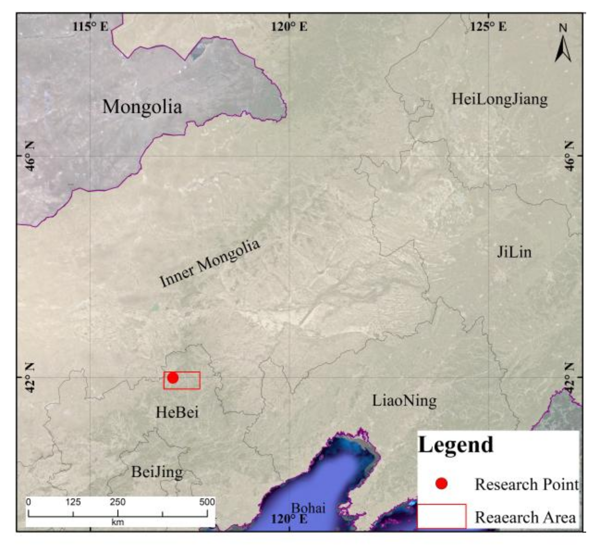
2.1. Study Area

The study area was located in the upstream region of Luan River—Beigou Forest Farm in Hebei Province (41°50′ N, 117°35′ E) (Figure 1). It was also located in the combination of the three major mountains in Northern China (Yinshan Mountain, Daxinganling Mountain, and Yanshan Mountain), where the large-area plantation not only reserved the water source of downstream Panjiakou reservoir and Luan River, but also regulated the sand-wind weather of Beijing [17,26]. This area is located in the Rocky Mountain Area of Northern China, and is characterized by a continental monsoon climate, with an annual average temperature of −1.4 °C to 4.7 °C, an average annual precipitation of 380 to 560 mm, and an average annual evaporation of 1462.9 to 1556.8 mm. The ≥0 °C annual accumulated temperature is 2180 °C and the frost-free period is 67–128 d [17]. The mountain brown soil develops under the natural secondary forest with deep topsoil [27]. The natural slope ranges from 1:150 to 1:350 with the altitude ranging between 750 m and 1829 m. The whole area of Beigou Forest Farm is 5428.8 hectares, including 1485.4 hectares of natural forests and 1180.5 hectares of artificial forests. There are four natural vegetation types; coniferous forest, broad-leaved deciduous forest, deciduous broad-leaved shrub, and subalpine meadow. Artificial forest species include Larix principis-rupprechtii, Pinus tabulaeformis, Betula platyphlla, and Populus davidiana; main shrubs include Corylus mandshuria, Spiraea pubescens, Onicera maackii, Weigela florida, and Rhododendron mucronulatum; and common herbs include Carex lancifolia, Phlomis umbrosa, and Thalictrum minus. Beigou Forest Farm was founded in 1956 and Mulan-Weichang Forestry Administration is responsible for its management [26,27,28,29,30,31].

2.2. Sample Plots and Field Survey

In 2009, we randomly selected Larix principis-rupprechtii plantation with five densities after thinning to set up five plots. Each plot had similar topography and soil conditions. The plots were marked as I, II, III, IV, and V, and their site factors—such as longitude, latitude, altitude, slope, aspect, etc.—were measured (Table 1). Plots I, II, III, and IV were pure L. principis-rupprechtii forest, and the proportion of L. principis-rupprechtii was 100%. Plot V was L. principis-rupprechtiiBetulaplatyphllaSuk mixed forest, and the proportions were 60% and 40%, respectively. Among these five plots, plot I and II were not thinned, while plots III, IV, and V were thinned with tending intensity of 45%, based on DBH (Diameter at Breast High) using the free thinning of regulations for tending of forests (GB/T 15781-1995) in 2006. Each plot was divided into squares of 10 m × 10 m as the investigation unit. Plot I and II had 6 squares each, plot III and IV had 9 squares each, and plot V had 25 squares. We used the grid method and GPS to locate all of the trees with DBH of >3 cm in the sample plots, and recorded the position of the trees. The distance between trees was indicated by the data from the Chinese NFI (National forest resource assessments and monitoring, commonly known as National Forest Inventories). We investigated the arborous layer, with each plot divided into quadrates (10 m × 10 m), as the investigation unit. All the trees with DBH of >3 cm in the sample plots were located. We then recorded DBH, branch height, crown width, height under branch, dominance, and stem form quality.

2.3. Data Processing

We selected four indexes to study the spatial structure of the plantation, including Mingling degree, Uniform angle index, Neighborhood comparison, and Opening degree. Mingling degree (M) referred to the proportion of different species among nearest neighbors and described the spatial isolation relationship of tree species [6]. Uniform angle index (W) indicated the complexity of stand spatial structure using the evenness among neighboring trees around the reference tree [6]. Neighborhood comparison (U) referred to the proportion of neighboring trees that were larger than the reference tree in all neighboring trees [6]. Opening degree (K) was a type of light environment index of the random sampling point [32,33,34].
The parameters of stand spatial structure, such as mingling degree, uniform angle index, neighborhood comparison, and opening degree, were calculated using Winkelmass 1.0. The formulas were as follows:
Mingling   degree :   M i = 1 4 j = 1 4 v i j
Uniform   angle   index :   W i = 1 4 j = 1 4 z i j
Neighborhood   comparison :   U i = 1 4 j = 1 4 K i j
Opening   degree :   K i = j = 1 4 ( D i j / H j )
where Vij, Kij, and Zij are discreteness variables, and are set as different values according to the following criteria: when reference tree i and its neighboring tree j were different species, Vij = 1, otherwise, Vij = 0; when the neighbor tree j was larger than the reference tree i, Kij = 1, otherwise, Kij = 0; when the angle a of the neighboring tree j was smaller than a0 (a0 = 72°), Zij = 1, otherwise, Zij = 0 [27]; Dij is the distance between the reference tree i and its neighboring tree j, Hj is the height of the neighboring tree j [35,36,37].
The values of Mingling degree (M) included 0.00, 0.25, 0.50, 0.75, and 1.00, representing zero degree, weak degree, moderate degree, strong degree, and extremely strong degree. The values of Uniform angle index included 0.00, 0.25, 0.50, 0.75, and 1.00. The stand-level distribution pattern was random, cluster, and uniform distribution when the average W ( W ¯ ) belonged to [0.475, 0.517], above 0.517, and lower than 0.517, respectively [10]. The values of Neighborhood comparison included 0.00, 0.25, 0.50, 0.75, and 1.00, representing superiority, sub-superiority, under the homogeneous, inferior, and absolute inferiority [9]. The values of Opening degree included [0, 0.2], [0.2, 0.3], [0.3, 0.4], [0.4, 0.5], and [0.5, ∞], denoting five spatial growth conditions of trees: seriously insufficient, slight insufficient, insufficient, sufficient, and strongly sufficient, respectively [32,33,34].
The M, W, U, and K can describe the stand spatial structure from the perspective of interspecific isolation, horizontal distribution, and tree height and growth space, respectively. However, it may still be difficult for forest managers to determine which level of reserve density can achieve a complicated spatial structure of the plantation, and therefore evaluate the overall effect of thinning. Thus, in order to develop a rapid and practical evaluation method, a composite structure index (Ci) was proposed based on the above results.
C i = a × M i + b × W i + c × U i + d × K i = a × 1 4 j = 1 4 v i j + b × 1 4 j = 1 4 Z i j + c × 1 4 j = 1 4 k i j + d × 1 4 j = 1 4 ( D i j / H j )
Ci is the overall complexity of the stand spatial structure, ranging between 0 and 1; a, b, c, and d represent the weights of Mi, Wi, Ui, and Ki, respectively, when describing the stand spatial structure. Although the weights of the variables should be considered carefully [32], little guidance can be drawn from the literature on how to assign weights to different variables of stand structural diversity [1]. However, a, b, c, and d were weighted based on the relative importance of each indicator in evaluating the complexity of forest spatial structure in this study. Their values were 0.10, 0.20, 0.30, and 0.40, denoting less important, important, more important, and very important, respectively.
All of the data were analyzed using a one-way ANOVA procedure and multiple comparison (p < 0.05).

3. Results

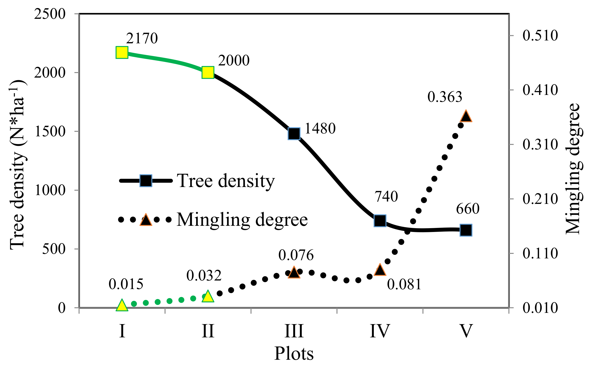
3.1. Effects of Thinning on Mingling Degree of Stand

The M of L. principis-rupprechtii plantation increased with the decreasing densities after thinning (Table 2 and Table 3, Figure 2). The M of plots I–IV were 0.015, 0.031, 0.076, and 0.081, respectively, which belong to the range of 0.00 to 0.25 and close to zero mix; the proportion of trees in zero mix was as high as 93.9%, 92.9%, 78.8%, and 77.4%, and a few were weak and extremely strong mix, with a severe lack of moderate and strong mixed types. With the increase of densities after thinning, the zero mix plantation increased gradually, while weak and extremely strong mix forests decreased. The results of pure L. principis-rupprechtii plantation are consistent with the results of Yong L, TAN Yangxin [38,39].
The interspecific isolation within L. principis-rupprechtiiBetula platyphylla mixed forest (V) was significantly higher than that of pure L. principis-rupprechtii (I–IV), and the overall M was 0.363, belonging to the transitional type between the weak and extremely strong types. The differentiation of the individual mixed status was more serious. The M decreased from zero to extremely strong mingling degree, and the trees with extremely strong mingling were very scarce, only accounting for 5.2% of the total. The results of L. principis-rupprechtiiBetula platyphylla mixed forest had good consistency with those of Zhang E L. et al. [40,41]. M increased slightly, with plant density decreasing, in the non-thinned plantation, while M increased significantly, with plant density decreasing, in the thinned plantation (non-thinned plots are highlighted in color in Figure 2). The reason was that thinning changed the spatial distribution relationship of the nearby trees, which resulted in the changes of M.
Overall, Mingling degree increased with the decrease of tree densities, and two groups of plots were clearly identified: although the thinning effect was an increase of the M index in the pure plantations (from plots I and II to III and IV), the results showed significantly lower values than in the mixed plantation.

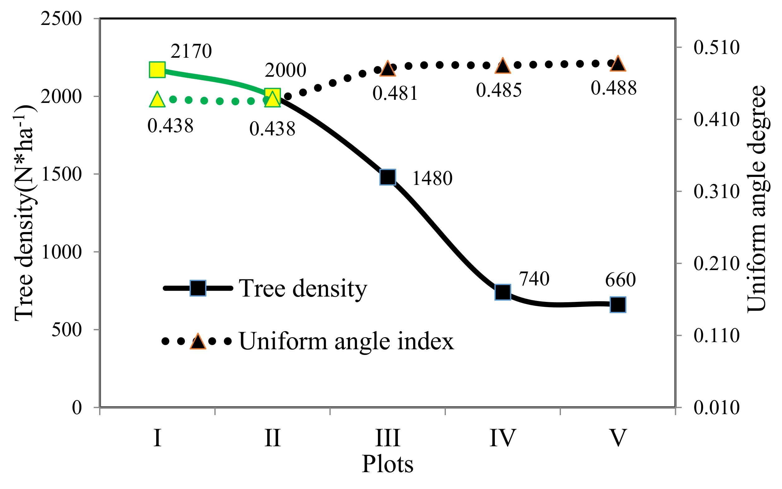
3.2. Effect of Thinning on the Distribution of Uniform Angle Degree

The uniform angle index of L. principis-rupprechtii plantation increased with the decreasing tree densities after thinning, and there was no significant difference (p > 0.05) between L. principis-rupprechtiiBetula platyphylla mixed forest and pure L. principis-rupprechtii forest (Table 2 and Table 3, Figure 3). The W of plot I and plot II with densities were [0.439, 0.438 < 0.475], respectively, and the stand’s horizontal distribution was uniform. The uniform angle indexes of plots III, IV, and V with densities were 0.481, 0.484, and 0.487 ∊ [0.475, 0.517], respectively, indicating that the stand’s horizontal distribution was random. However, the extent of random distribution was so low that it was close to an even distribution. The relative accuracy of the tree distribution was judged to be uniform, random, or regiment, which is consistent with the studies of Gadow K and others [32,33]. The W in five densities showed that the majority within the communities were distributed randomly (Figure 3). Wi = 0.5 meant the ratio of the tree number was close to or more than 0.5; the number of uniformly distributed individual trees (Wi = 0.25) was significantly larger than that of individual trees in a clumped distribution (Wi = 0.75). In contrast, the individual trees in a significantly even distribution (Wi = 0) or a clumped distribution (Wi = 1) were extremely rare [32,33,34]. Among the trees, there were three kinds of distribution patterns: random, cluster, and uniform distribution [42,43,44]. For the whole community, thinning could effectively promote the evolution from uniform to random distribution within the plantation. W increased slightly, with plant density decreasing, in the non-thinned plantation, while W increased significantly, with plant density decreasing, in the thinned plantation. (non-thinned plots are highlighted in color in Figure 3). The uniformity changes of nearby trees, caused by thinning, may change the stand spatial structure and result in the change of W. The most important result was that the W index was sensible to thinning and was able to detect its effects. In particular, as highlighted in Table 3, there were two groups of plots (I–II and III–IV–V), meaning non-thinned and thinned plots.

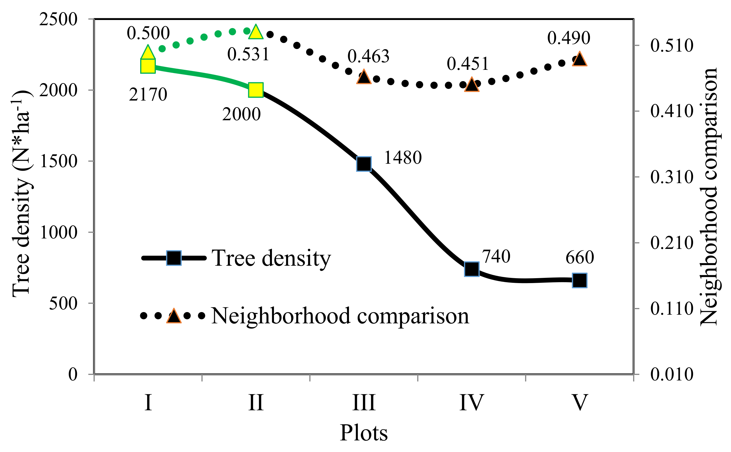
3.3. Effect of Thinning on Neighborhood Comparison

DBH was calculated as the index of neighborhood comparison. Table 2 and Table 3, Figure 4 showed that the U of Larix principis-rupprechtii plantation under five densities after thinning were 0.500, 0.531, 0.462, 0.452, and 0.489 respectively, and the stand was under the homogeneous state. With the decreasing densities after thinning, the response of U became more complicated. Within sample plot I–IV, U decreased with the decrease of densities after thinning, and the competition density among stand individual decreased with the decreasing density after thinning. But the stand density in sample plot IV was greater than that in sample plot II, while U had the opposite trend, indicating that U was a spatial structure parameter associated with the DBH of reference trees, as shown by the equation. Although the densities after thinning in sample plots IV and II were close, DBH in sample plot IV was less than that in sample plot II, which greatly reduced the competitive pressures of trees in sample plot IV. The densities after thinning in Larix principis-rupprechtiiBetula platyphylla mixed forest (V) was the smallest. Two groups of results were concluded. U in non-thinned plots (I, II) (showing a sub-superior structure, U > 0.5) was significantly higher than that in thinned plots (III, IV, V) (showing a sub-superior structure, U > 0.5), and higher in mixed plot (V) than in thinned pure plots (III, IV). The tree density seems to not be an explanatory variable for the U index.
The composition proposition changes of nearby trees, caused by thinning, ultimately resulted in the changes of U. These results were consistent with the research of Hui GY.et al. [45,46]. The U mainly depends on the initial growth status of trees and the competitive ability of trees [47,48,49].

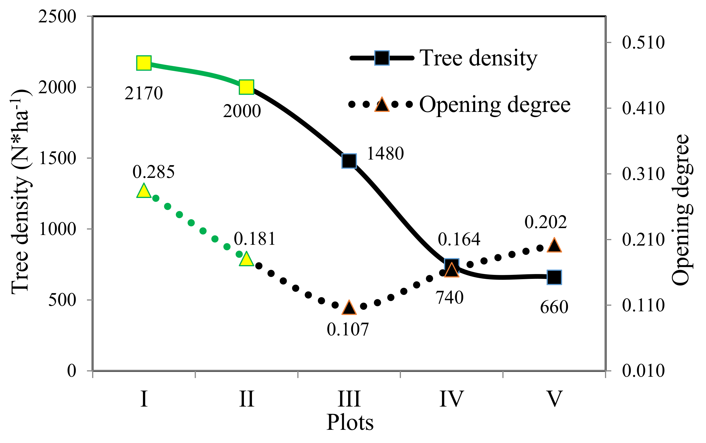
3.4. Effect of Thinning on Opening Degree

Table 2 and Table 3, Figure 5 show that the opening degrees of L. principis-rupprechtii plantation under five densities after thinning were 0.285, 0.181, 0.107, 0.164, and 0.202, respectively, indicating that the stand was seriously insufficient and their growth was significantly inhibited. For individual trees, the vast majority grew in a seriously restricted space. On five sample plots, except for the fact that 30.6% of stands in plot I had basic growth space, all other plots lacked basic growth space. In particular, the proportion of inadequate space in plot III reached nearly 100%. With the increasing densities after thinning, there was no significant variation pattern for K, as in the case of U. It appears that the thinning reduced the structural diversity in the plantation. The growth of forest trees changed regularly with the regulation of K, the results were similar to the results of Riitters K. and other studies on the growth of forest trees [50,51]. Equation (4) shows that the K was not only associated with DBH of the reference tree, but also with the height of neighboring trees. In general, larger densities after thinning resulted in greater competitive intensity among trees, thereby restricting the development of DBH and height. On the contrary, smaller densities after thinning led to lower competitive intensity among trees and facilitated the development of DBH and height. The effect of thinning was to leave the best trees, eliminating the small differences in the forest. K increased slightly, with plant density decreasing, in the non-thinned plantation, while it increased significantly, with plant density decreasing, in the thinned plantation. (non-thinned plots are highlighted in color in Figure 5). Therefore, the limiting factors of K and their variation were more complicated when compared with U.

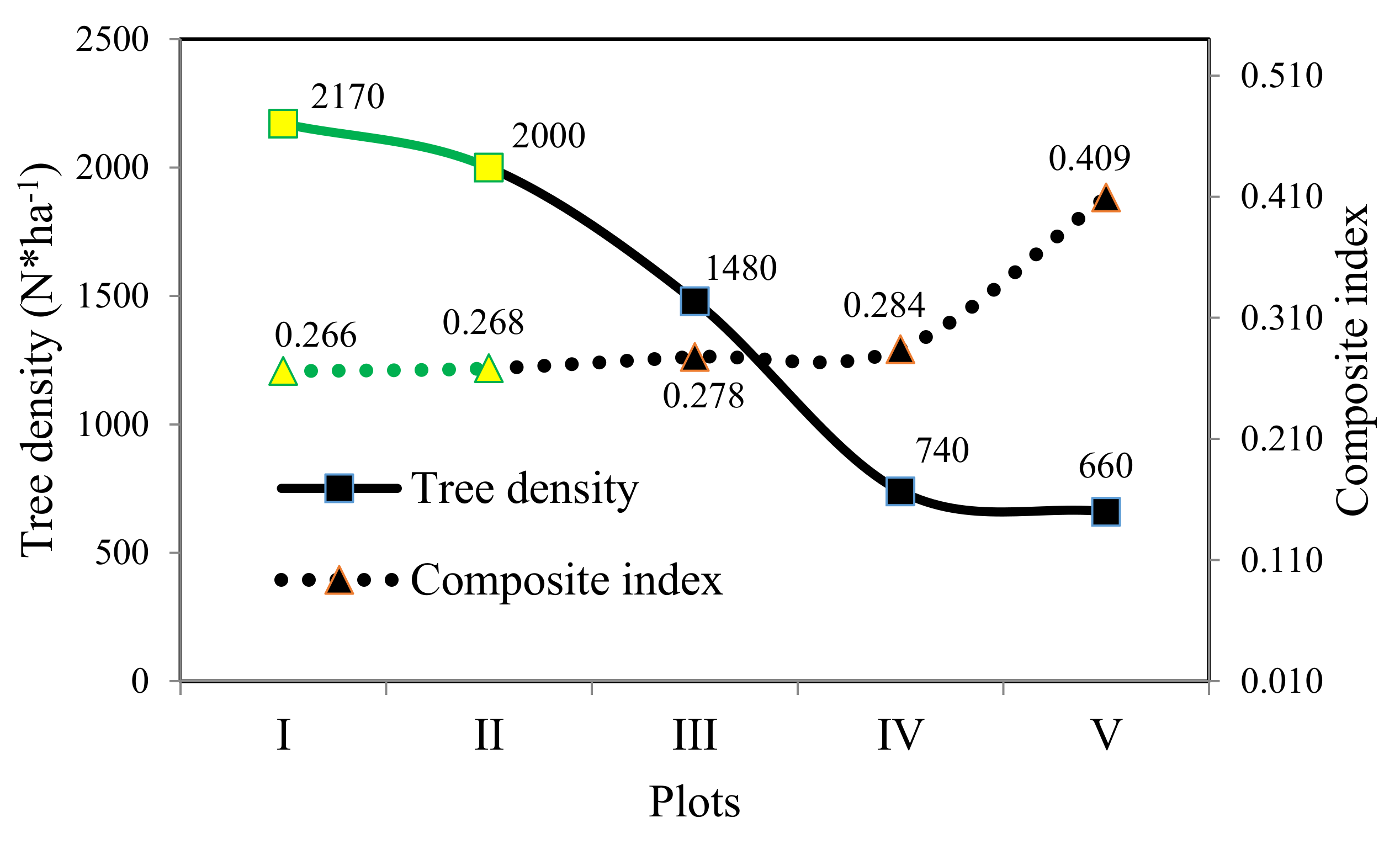
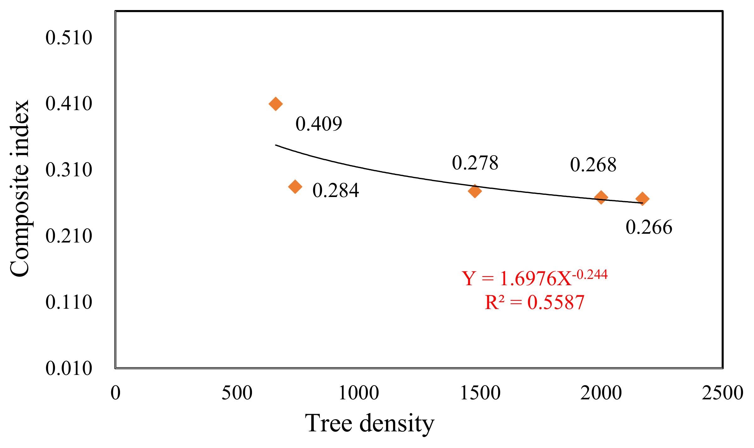
3.5. Multiple Comparison and Construction of Composite Spatial Structure Index

The variance analysis and multiple comparison of M, W, U, and K showed that M between plots I–IV (pure plantation) and plot V (mixed plantation) all had significant differences (p < 0.05), while M among plots I–IV (pure plantation) had no significant differences (p > 0.05). However, among four pure plots I–IV, M of thinned plots I and II were lower than that of non-thinned plots III and IV, and no significant differences were observed. W in plots I–IV had no significant differences, whether pure plantation or mixed plantation. W of thinned plots I and II were lower than that of non-thinned plots III–V, and no significant differences were observed. U between plots I and III–IV, U between plots II and III–V, and U between plots V and III–IV all showed significant differences. U between plots I and II, as well as between plots III and IV, had no significant differences. In the perspective of thinning and non-thinning, except for non-thinned plot I and thinned plot IV, which had no significant differences, U of the other thinned and non-thinned plots had significant differences. In four pure plantation plots, non-thinned plots I and II had similar U, while thinned plots III and IV had similar U. The comparisons of K showed that, except for plot II and V, which had no significant differences, all of the other plots had significant differences. Among the non-thinned plots, plot I and II had significant differences, and plot V and III–IV also showed significant differences (Table 3). This was the reason that the four indexes—namely, M, W, U, and K—all considered the nearby trees. However, because plots I–IV were the same tree, they experienced the same environment under both thinning and non-thinning, although there were no significant differences among the decreasing tree density. This showed that there was some limitation on using any single one of the four indexes to express the differences of stand spatial structure.
The above results showed that Mi and Wi in Larix principis-rupprechtii plantation increased with the decreasing densities after thinning, and that the increasing extent of Mi was larger than that of Wi. Ui showed a decreasing trend. In addition, the action of more complex factors that influenced Ki resulted in no significant variation rule for Ki under the densities after thinning. These findings indicated that Mi had the greatest impact, followed by Wi, Ui, and Ki, such that the weights of a, b, c, and d were 0.10, 0.20, 0.30, and 0.40, respectively. Figure 6 showed that Ci in Larix principis-rupprechtii plantation increased with the decreasing densities after thinning. This means that the stand spatial structure became more complex as the reserve intensity increased. The comparison of results of Ci showed that for thinning and non-thinning, Ci of non-thinned plots I and II were similar, Ci started increasing from plot III–IV, and non-thinned plot I had significant differences with both plots II and V. For the stand composition, pure plantation plots I–IV had significant differences with plot V, but no significant differences among themselves. Figure 7 shows that Ci had the same trend as four single indexes. Thus, Ci can be considered as a simple and rapid evaluation indicator for plantation managers to determine the effect of thinning on stand spatial structure. Moreover, managers can assess the suitability of stand thinning intensity using Ci, which also provides a reference to optimize the plantation management of stand structure in the future.

4. Discussion

4.1. Response of Forest Spatial Structure to Thinning

Structure determines function, according to the system theory [35]. This means that the system functions can only be given full play when a good system structure is maintained [36]. Thinning improves the stand volume growth rate, tree growth, and crown development of the remaining trees. Thinning opens up new niches in forest communities; optimizes the spatial structure, and ultimately relieves the competitive intensity among trees; promotes succession; and improves the forest health. Only healthy and stable forest communities can fully perform their ecological, social, and economic functions, as well as increase the forest structural diversity and improve the stability of the forest ecosystem [52,53]. However, thinning also affects the remaining trees in dimensions that may vary according to the length of the periods after thinning (short-term or long-term), thinning intensity, and environmental conditions. Previous studies have demonstrated a relationship of thinning with growth and yield [54,55]. This suggested that space structure increased after thinning and decreased competition among species for resources (e.g., soil, water, and nutrients), which is beneficial for tree growth. Thus, the above tree growth parameters increased.
Stand spatial structure indicators are defined as indexes to describe the features of forest spatial structure, which not only plays an important role in analyzing and controlling the forest structure and function relationship, but also is the focus, and difficult, point in the research of stand spatial structure [56,57]. This study was based on the analysis of the research status of stand spatial structure unit; it summed up the research trends of stand spatial structure indicators from Mingling degree, Uniform angle index, Neighborhood comparison, and Opening degree; and it built a composite structure index (Ci) to assess the effect of thinning. The results showed that thinning affected the spatial structure of L. principis-rupprechtii plantation to different degrees. With the decreasing densities after thinning, M and W increased, but the mixed degree was generally low and the randomness of horizontal distribution was still poor, resulting in zero mix in the vast majority of trees. The trees in moderate, strong, and extremely strong mixed status were few, and the horizontal distribution under five densities after thinning was uniform or near-uniform random. U and K fluctuated with densities after thinning: U showed a decreasing trend, while K had an increasing trend. This indicated that thinning could alleviate the competitive intensity between trees. However, the detailed response mechanisms among U, K, stand density, DBH, and height were more complex, and require further study. Additionally, because of the longer natural succession process in forest vegetation, proper human disturbance is recommended, such as the introduction of native species and broad-leaf species and the creation of mixed forests to accelerate the recovery and reconstruction of the plantation structure.

4.2. Determination and Evaluation of Thinning Intensity in Structure-Based Forest Management

Most of the thinning operations in China are based on traditional forest management theory, which mainly focuses on growth indexes, such as DBH and height, while ignoring the stand spatial structure, resulting in a poor management effect. With the traditional thinning mode, a passive response of stand spatial structure to thinning greatly restricts the production and eco-efficiency of thinning operations. Thinning operations based on modern structured forest management advocated the business philosophy that included tree-oriented, nurturing-based, and ecological priority to foster a healthy and stable forest. Furthermore, according to the principle that structure determines function, as well as the succession process of natural forest, the quantitative analysis and management methods of spatial structure should be advocated based on the relationship among the adjacent trees. This effectively avoids the operating risks, greatly enhances the effects of thinning, and precisely adjusts the stand structure. Therefore, thinning can be a simple, sustainable method for scientific forest management [58].
A study on the stand spatial structure is one of the core contents in structure-based forest management. The purpose of stand management is to find a reasonable representation of spatial structure, including appropriate parameters, and effectively rebuild the spatial distribution pattern [59]. Many analysis methods for stand spatial structure have been discussed, such as the combination of remote sensing (RS) and Geographic Information Systems (CIS) [60], statistical analysis of community structure characteristics [61,62,63,64,65], and the establishment of an evaluation model and indexes [63,64,65,66,67]. Although the new spatial structure indicators—including M, W, U, and K—provide a more detailed analysis for stand spatial structure than common indicators, it is still difficult for forest managers to quickly determine which level of stand spatial structure is more sophisticated and beneficial for maintaining forest ecosystem functions [65,66,67]. Additionally, it is important for managers to consider the problem of how to quickly and efficiently evaluate the effect of management measures, such as thinning on the plantation’s spatial structure, when optimizing the structure. Therefore, a composite structure index (Ci) was proposed according to the effect of five reserve intensities on L. principis-rupprechtii plantation structure. The results suggested that Ci is feasible as an indicator.
Using Mingling degree, Uniform angle index, Neighborhood comparison, and Opening degree indexes as “input” and the forest spatial structure as “output”, the production function of forest spatial structure is constructed. At present, there are some shortcomings in the method of calculating the spatial structure of forest stand with four kinds of single index. However, when we generate a weighted comprehensive index, we can increase the complementarity among the indicators to offset these shortcomings as much as possible. Therefore, the comprehensive index Ci, built based on M, W, U, and K, provided a more convenient and useful tool for forest management. Since Ci was established on the basis of this study, it needs to be further studied in other areas.

5. Conclusions

Thinning affects the spatial structure of L. principis-rupprechtii plantation to different degrees. Mingling degree increased with the decrease of tree densities in both pure L. principis-rupprechtii plantation and L. principis-rupprechtii–Betula platyphylla mixed forest. The uniform angle index of L. principis-rupprechtii plantation increased with the decreasing densities after thinning, and there was no significant difference between the mixed forest and pure forest. The stand’s horizontal distribution of L. principis-rupprechtii plantation was uniform, while that of L. principis-rupprechtii–Betula platyphylla mixed forest was random. U of Larix principis-rupprechtii plantation under five densities after thinning was under the homogeneous state. With the decreasing densities after thinning, the response of U became more complicated. The opening degree of L. principis-rupprechtii plantation indicated that the stand was seriously insufficient and their growth was significantly inhibited. With the increasing densities after thinning, there was no significant variation pattern for K, as in the case of U. K was associated not only with DBH of the reference tree, but also with the height of neighboring trees. The limiting factors of K and their variation were more complicated when compared with U. Overall, with the decreased densities after thinning, mingling degree and uniform angle index increased, but the mix degree was generally low and the randomness of the horizontal distribution was still poor. The horizontal distribution under five densities after thinning was uniform or near-uniform random. The neighborhood comparison and opening degree fluctuated with densities after thinning: neighborhood comparison showed a decreasing trend, while opening degree had an increasing trend, indicating that thinning could alleviate the competitive intensity between trees.
From the point of view of thinning or non-thinning, in the non-thinned plantations (plots I and II), M, W, and U showed the same trends—that is, they increased with the decreased tree density—while K showed the opposite trend. In the thinned plantation, M, W, U, and K increased, with strengthened thinning intensity, and showed the same trends. Overall, in both the thinned/non-thinned plantation and the pure/mixed plantation, all of the above four indexes increased, with plant density decreased, and especially, increased significantly with strengthened thinning intensity. This showed that plant density had significant effects on the different structure indexes. Thus, thinning with decreasing plant density changed the stand spatial structure. The changes caused by thinning also could be reflected by spatial structure indexes, M, W, U, and K (the correlations with the tree density were 0.54, 0.79, 0.93, and 0.94, respectively), which verified our first hypothesis that there was a positive relationship between the thinning intensity and spatial structure indexes. M, W, U, and K showed the same trends after thinning, suggesting our second hypothesis was feasible, that is, the composite spatial structure index (Ci), based on M, W, U, and K, can reflect the complexity of stand spatial structure.
The Ci of L. principis-rupprechtii plantation increased with the decreasing densities after thinning. That is, stand spatial structure became more complex as thinning intensity increased, suggesting that Ci can be used as a simple and rapid evaluation indicator for plantation managers to determine the effect of thinning on stand spatial structure. Moreover, managers can assess the suitability of stand thinning intensity using Ci, which also provides a reference to optimize the plantation management of stand structure in the future. Since the parameters used for calculating Ci were estimated from the results of this study, the index is site-specific. Further studies would be necessary to improve the applicability of the proposed index.

Acknowledgments

This work was funded by the Fundamental Research Funds for the Central Universities (No. 2015ZCQ-SB-02) and the National Natural Science Foundation of China (31270749).

Author Contributions

Guodong Ding and Guanglei Gao conceived and designed the experiments; Shengxing Ye, Yanfeng Bao and Yundong Liu performed the experiments; Guanglei Gao and Shengxing Ye analyzed the data; Shengxing Ye and Zhirong Zheng wrote the paper; Zhirong Zheng charted the map of study area and revised the manuscript.

Conflicts of Interest

The authors declare no conflict of interest.

References

  1. Hui, G. Studies on the application of stand spatial structure parameters based on the relationship of neighborhood trees. J. Beijing For. Univ. 2013, 35, 1–8. [Google Scholar]
  2. Pretzsch, H. Analysis and modeling of spatial stand structures Methodological considerations based on mixed beech-larch stands in Lower Saxony. For. Ecol. Manag. 1997, 97, 237–253. [Google Scholar] [CrossRef]
  3. Pastorella, F.; Paletto, A. Stand structure indices as tools to support forest management: An application in Trentino forests. J. For. Sci. 2013, 59, 159–168. [Google Scholar] [CrossRef]
  4. Hui, G.Y.; Hu, Y.B. Measuring Species Spatial Isolation in Mixed Forests. For. Res. 2001, 14, 23–27. [Google Scholar]
  5. Hui, G.Y.; Klaus, V.G.; Matthias, A. A New Parameter for Stand Spatial Structure—Neighbourhood Comparison. For. Res. 1999, 12, 1–6. [Google Scholar]
  6. Hui, G.Y.; Klaus, V.G.; Matthias, A. The neighborhood pattern—A new structure parameter for describing distribution of forest tree potation. Sci. Silv. Sin. 1999, 35, 37–42. [Google Scholar]
  7. Hu, Y.B.; Hui, G.Y. A Discussion on Forest Management Method Optimizing Forest Spatial Structure. For. Res. 2006, 19, 1–8. [Google Scholar]
  8. Zhong, J.F.; Liu, D.L.; Zheng, X.X. The Quantitative Research Progress of Water Conservation Forest’s Structure and Function. Mod. Agric. Sci. 2009, 16, 110–112. [Google Scholar]
  9. Oliver, C.D. A landscape approach: Achieving and maintaining biodiversity and economic productivity. J. For. 1992, 90, 20–25. [Google Scholar]
  10. Franklin, J.F.; Spies, T.A.; Pelt, R.V.; Carey, A.B.; Thornburgh, D.A.; Berg, D.R.; Lindenmayer, D.B.; Harmon, M.E.; Keeton, W.S.; Shaw, D.C.; et al. Disturbances and structural development of natural forest ecosystems with silvicultural implications, using Douglas-fir forests as an example. For. Ecol. Manag. 2002, 155, 399–423. [Google Scholar] [CrossRef]
  11. Carey, A.B.; Elliot, C.E.; Lippke, B.R.; Sessions, J.; Chambers, C.J.; Oliver, C.D.; Franklin, J.F.; Raphael, M.G. Washington Forest Landscape Management Project—A Pragmatic, Ecological Approach to Small Landscape Management; Report No.2; Washington State Department of Natural Resources: Olympia, WA, USA, 1996.
  12. Tang, M.P. Study on Forest Spatial Structure Analysis and Optimal Management Model; Beijing Forestry University: Beijing, China, 2003. [Google Scholar]
  13. An, H.; Hui, G.; Zheng, X.; Zhang, T.; Hu, Y.; Meng, Q. Study on the spatial structure of broad-leaved Korean pine forest in the different growth stage. Acta Sci. Nat. Univ. Neimongol 2005, 36, 714–718. [Google Scholar]
  14. FAO Yearbook of Forest Products; FAO: Rome, Italy, 2015.
  15. State Forestry Administration. The Results of Seventh National Forest Resources Inventory. 2010. Available online: http://www. Forestry.gov.cn/partal/main/s/65/content-326341.html (accessed on 4 May 2010).
  16. State Forestry Administration of Forest Resources Management. The seventh national forest resources inventory and the status of the forest resources. For. Resour. Manag. 2010, 39, 1–8. [Google Scholar]
  17. Gao, G.L.; Ding, G.D.; Xiao, M.; Zhang, L.L.; Ren-Meng, L.; Zhang, X.; Li, W.; Liu, Y. A study on stand visualization of artificial mixed forests. Bull. Soil Water Conserv. 2012, 32, 158–162. [Google Scholar]
  18. Ma, L.Y.; Li, C.Y.; Wang, X.Q.; Xu, X. Effects of Thinning on the Growth and the Diversity of Undergrowth of Pinus tabulae formis Plantation in Beijing Mountainous. Sci. Silv. Sin. 2007, 43, 1–9. [Google Scholar]
  19. Zheng, L.F.; Zhou, X.N. Dynamics Effects of Selective Cutting Intensity on the Species Composition and Diversity of Natural Forest. J. Mount. Sci. 2008, 26, 699–706. [Google Scholar]
  20. An, Y.; Ding, G.D.; Liang, W.J.; Gao, G.L.; He, Y.; Wei, B.; Bao, Y.; Bao, B. Effects of Tending and Thinning on the Community Stability of Pinus tabulae formis Plantation in Rocky Mountain Area of Northern China. J. Sichuan Agric. Univ. 2012, 30, 12–17. [Google Scholar]
  21. Zhu, J.J.; Li, F.Q.; MatsuzakiI, T.; Gonda, Y. Influence of thinning on regeneration in a coastal Pines thunbergii forest. Chin. J. Appl. Ecol. 2002, 13, 1361–1367. [Google Scholar]
  22. Bréda, N.; Granier, A.; Aussenac, G. Effects of thing on soil and tree water relations, transpiration and growth in an oak forest (Quercuspetraea (Matt.) Liebl). Tree Physiol. 1995, 15, 295–306. [Google Scholar] [CrossRef] [PubMed]
  23. An, Y.; Ding, G.D.; Liang, W.J.; Gao, G.L.; He, Y.; Wei, B.; Bao, Y.; Bao, B. Effects of Thinning on the Growth and the Development of Undergrowth of Pinus tabulae formis Plantation in Rocky Mountain Area of North China. Res. Soil Water Conserv. 2012, 19, 86–90. [Google Scholar]
  24. Liu, Q. Ecological Problems of Subalpine Coniferous Forest in the Southwest of China. World Sci. Technol. R&D 2001, 23, 63–69. [Google Scholar]
  25. Hu, D.; Wang, R. Exploring eco-construction for local sustainability: An eco-village case study in China. Ecol. Eng. 1998, 11, 167–176. [Google Scholar] [CrossRef]
  26. Ren, L.N.; Wang, H.Y.; Ding, G.D.; Gao, G.L.; Yang, X.J. Effects of Pinus tabulaeformis Carr. plantation density on soil organic carbon and nutrients characteristics in rocky mountain area of northern China. Arid Land Geogr. 2012, 35, 456–464. [Google Scholar]
  27. Yao, W.; Hu, J.; Yang, X. Physical Properties of Soil Water in Mixed Forest of Larix principis-rupprechti in Northern Mountain of Hebei Province. Prot. For. Sci. Technol. 2016, 155, 1–3. [Google Scholar]
  28. Tang, J.W.; Qi, Y.; Xu, M.; Misson, L.; Goldstein, A.H. Forest thinning and soil respiration in a ponderosa pine plantation in the Sierra Nevada. Tree Physiol. 2005, 25, 57–66. [Google Scholar] [CrossRef] [PubMed]
  29. He, Y.; Ding, G.D.; Liang, W.J.; Zang, Y.T.; Gao, G.L.; An, Y. Influence of stand density on water-holding characteristics of litter layer. J. Northwest A&F Univ. 2012, 40, 68–72. [Google Scholar]
  30. Zhao, J.C.; Kong, Z.P. Flora of Mulan Weichang in Hebei; Science Press: Beijing, China, 2008; Volume 1, pp. 68–72. ISBN 9787030232151. [Google Scholar]
  31. Gao, G.L.; Ding, G.D.; Zhang, J.Y.; Ren, L.N.; Zang, Y.T.; Liang, W.J. Spatial Structural Characteristics of Natural Secondary Forest in Rocky Mountain Area of Northern China. Bull. Soil Water Conserv. 2011, 31, 81–85. [Google Scholar]
  32. Gadow, K. Zur Bestandesbeschreibung in der Forsteinrichtung. Forst Holz 1993, 48, 601–606. [Google Scholar]
  33. Dong, L.; Liu, Z.; Ma, Y.; Ni, B.; Li, Y. A new composite index of stand spatial structure for natural forest. J. Beijing For. Univ. 2013, 35, 16–22. [Google Scholar]
  34. Hu, Y.; Bo, H.Y.; Bo, X.H. Structured Forest Management; China Forestry Publishing: Beijing, China, 2007; Volume 1, pp. 56–60. ISBN 9787503847639. [Google Scholar]
  35. Hao, Y.Q.; Wang, J.X.; Wang, Q.H.; Sun, P.; Pu, C.L. Preview of Spatial Structure of Cryptomeriafortunei Plantation after Stand Improvement. Sci. Silv. Sin. 2006, 42, 8–12. [Google Scholar]
  36. Gao, G.L.; Ding, G.D.; Ren, L.N.; Zang, Y.T.; Liang, W.J. Application of spatial competition index to the natural secondary forest of rocky mountain area in Northern China. J. Arid Land Resour. Environ. 2012, 26, 134–138. [Google Scholar]
  37. Lv, Y.; Tan, Y.; Lv, F.; Li, X.; Zhang, J. Research on Thinning Intensity of Natural Secondary Forest—A Case of Schima superba Secondary Forest of Qingshigang Forest Farm. For. Resour. Manag. 2013. [Google Scholar] [CrossRef]
  38. Tan, Y. The Thinning Intensity Research of Natural Secondary Forest Based on Cutting Index; Central South University of Forestry and Technology: Changsha, China, 2014. [Google Scholar]
  39. Zhang, E.L. Study on Route of Natural Secondary Forest Management. J. Anhui Agric. Sci. 2015, 43, 77–78. [Google Scholar]
  40. Wang, A.; Liu, B. Study on Manage of Natural Secondary Forest. Jiangxi For. Technol. 2000, 3, 1–4. [Google Scholar]
  41. Lei, X.D.; Tang, S.Z. Indicators on structural diversity within-stand: A review. Sci. Silv. Sin. 2002, 38, 140–146. [Google Scholar]
  42. Pan, Y.; Birdsey, R.A.; Phillips, O.L.; Jackson, R.B. The Structure, Distribution, and Biomass of the World’s Forests. Annu. Rev. Ecol. Evol. Syst. 2013, 44, 593–622. [Google Scholar] [CrossRef]
  43. Ren, H.; Jian, S.; Lu, H.; Zhang, Q.; Shen, W.; Han, W.; Yin, Z.; Guo, Q. Restoration of mangrove plantations and colonisation by native species in Leizhou bay, South China. Ecol. Res. 2008, 23, 401–407. [Google Scholar] [CrossRef]
  44. Hui, G.Y.; Hu, Y.B.; Zhao, Z.H. Further discussion on “Structure-based Forest Management”. World For. Res. 2009, 22, 14–19. [Google Scholar]
  45. Huang, L.; Huo, Y.; Jin, H.; Li, N. Relationship between Neighborhood Comparison and Diameter Growth of Secondary Poplar-birch Forest in the Mountains of North Hebei. For. Resour. Manag. 2014. [Google Scholar] [CrossRef]
  46. Gao, G.L.; Xin, Z.B.; Ding, G.B.; Li, C.C.; Zhang, J.Y.; Liang, W.; An, Y.; He, Y.; Xiao, M.; Li, W. Forest health studies based on remote sensing: A review. Acta Ecol. Sonica 2013, 33, 1675–1689. [Google Scholar]
  47. Hao, Z.; Zhang, J.; Song, B.; Ye, J.; Li, B. Vertical structure and spatial associations of dominant tree species in an old-growth temperate forest. For. Ecol. Manag. 2007, 252, 1–11. [Google Scholar] [CrossRef]
  48. Ma, L.K. Forest vegetation and soil succession the natural process of change. In Proceedings of the TEP Seminar XIII: Trees, Roots, Fungi, Soil (Part 2), Bristol, UK, 20 June 2009. [Google Scholar]
  49. Riitters, K.; Wickham, J.; O’Neill, R.; Jones, B.; Smith, E. Global-scale patterns of forest fragmentation. Conserv. Ecol. 2000, 4, 1924–1925. [Google Scholar] [CrossRef]
  50. Wang, J.W.; Hou, M.M.; Huang, L.Y.; Zhang, J.; Zhou, H.-C.; Cheng, Y.-X. Phylogenetic and functional beta diversity in a broadleaved Korean pine mixed forest in Changbai Mountains, northeastern China. J. Beijing For. Univ. 2016. [Google Scholar] [CrossRef]
  51. Onaindia, M.; Ametzaga-Arregi, I.; Sebastián, M.S.; Mitxelena, A.; Rodríguez-Loinaz, G.; Peña, L.; Alday, J.G. Can understorey native woodland plant species regenerate under exotic pine plantations using natural succession? For. Ecol. Manag. 2013, 308, 136–144. [Google Scholar] [CrossRef]
  52. Li, J.; Zheng, X. The Forest Health Assessment Indicator System for the Water conservation Forests in Beijing Area. For. Resour. Manag. 2004, 1, 31–34. [Google Scholar]
  53. Yen, T.M.; Lee, J.S.; Li, C.L.; Chen, Y.T. Aboveground biomass and vertical distribution of crown for Taiwan red cypress 20 years after thinning. Dendrobiology 2013, 70, 109–116. [Google Scholar] [CrossRef]
  54. Yen, T.M. Relationships of Chamaecyparis formosensis crown shape and parameters with thinning intensity and age. Ann. For. Res. 2015, 58, 323–332. [Google Scholar] [CrossRef]
  55. Zhang, P.F.; He, W.R.; He, X.; Zhang, J.; Li, Y.M. An approach on forest spatial change in Xishuangbanna. Acta Geogr. Sin. 1999, 54, 139–145. [Google Scholar]
  56. McElhinny, C.; Gibbons, P.; Brack, C.; Bauhus, J. Fauna-habitat relationships: A basis for identifying key stand structural attributes in temperate Australian eucalypt forests and woodlands. Pac. Conserv. Biol. 2006, 12, 89–110. [Google Scholar] [CrossRef]
  57. Shu, Y.Q.; Lan, Z.R.; Chen, C.C. Analysis and Simulation of the time-varying property of Forest Spatial Data. Comput. Eng. 2005, 31, 27–29. [Google Scholar]
  58. Riitters, K.H. Downscaling indicators of forest habitat structure from national assessments. Ecol. Indic. 2005, 5, 273–279. [Google Scholar] [CrossRef]
  59. Segura, A.; Castaño-Santamaría, J.; Laiolo, P.; Obeso, J.R. Divergent responses of flagship, keystone and resource-limited bio-indicators to forest structure. Ecol. Res. 2014, 29, 925–936. [Google Scholar] [CrossRef]
  60. McElhinny, C.; Gibbons, P.; Brack, C. An objective and quantitative methodology for constructing an index of stand structural complexity. For. Ecol. Manag. 2006, 235, 54–71. [Google Scholar] [CrossRef]
  61. Hui, G.; Hu, Y. Application of Neighborhood Pattern in Forest Spatial Structure Regulation. For. Resour. Manag. 2006, 2, 31–36. [Google Scholar]
  62. Aguirre, O.; Hui, G.; Gadow, K.V.; Jiménez, J. An analysis of spatial forest structure using neighborhood-based variables. For. Ecol. Manag. 2003, 183, 137–145. [Google Scholar] [CrossRef]
  63. Yue, Y.J.; Yu, X.X.; Li, G.T.; Fan, D.X.; Ye, J.D. Spatial structure of Quercus mongolica forest in Beijing Songshan Mountain Nature Reserve. J. Appl. Ecol. 2009, 20, 1811–1816. [Google Scholar]
  64. Porté, A.; Bartelink, H.H. Modelling mixed forest growth: A review of models for forest management. Ecol. Model. 2002, 150, 141–188. [Google Scholar] [CrossRef]
  65. Canham, C.D.; Uriarte, M. Analysis of neighborhood dynamics of forest ecosystems using likelihood methods and modeling. Ecol. Appl. 2006, 16, 62–73. [Google Scholar] [CrossRef] [PubMed]
  66. Queenborough, S.A.; Burslem, D.F.; Garwood, N.C.; Valencia, R. Neighborhood and community interactions determine the spatial pattern of tropical tree seedling survival. Ecology 2007, 88, 2248–2258. [Google Scholar] [CrossRef] [PubMed]
  67. McElhinny, C.; Gibbons, P.; Brack, C.; Bauhus, J. Forest and woodland stand structural complexity: Its definition and measurement. For. Ecol. Manag. 2005, 218, 1–24. [Google Scholar] [CrossRef]
Figure 1. The location of the study area.
Sustainability 10 01250 g001
Figure 2. The effect of tree density on mingling degree. (Hereinafter the N*ha−1 refers to the tree number in per ha).
Sustainability 10 01250 g002
Figure 3. The effect of tree density on uniform angle degree.
Sustainability 10 01250 g003
Figure 4. The effect of tree density on neighborhood comparison.
Sustainability 10 01250 g004
Figure 5. The effect of tree density on opening degree.
Sustainability 10 01250 g005
Figure 6. The effect of tree density on the composite structure index.
Sustainability 10 01250 g006
Figure 7. The relationship between tree density and the composite structure index.
Sustainability 10 01250 g007
Table 1. General situation of the sample plots.
Sample PlotArea (m2)Tree Density (Tree Number⋅ha1)Mean Diameter at Breast High (cm)Average Height (m)Basal Area (m2⋅ha−1)Stand Age (a)Slope (°)Altitude (m)
I60021706.886.528.5140101233
II600200011.3310.0322.0040121293
III900148016.7420.0736.6840211370
IV90074020.0714.8724.0840211318
V250066019.1817.7825.3740211338
Table 2. Distributions of M, W, U, and K in different stand relative frequency distributions.
IndicatorValueSample Plot
IIIIIIIVV
M 0.000.9390.9290.7880.7740.296
0.250.0610.0540.1820.1940.252
0.500.0000.0000.0000.0000.209
0.750.0000.0000.0000.0000.191
1.000.0000.0180.0300.0320.052
M ¯ 0.0150.0320.0760.0810.363
W 0.000.0000.0000.0150.0320.000
0.250.4080.2860.1970.1940.244
0.500.4490.6790.6520.5810.600
0.750.1220.0360.1210.1940.122
1.000.0200.0000.0150.0000.035
W ¯ 0.4380.4380.4810.4850.488
U 0.000.1840.2140.2270.2260.200
0.250.2450.1250.2120.2260.217
0.500.1630.1960.2120.2260.191
0.750.2040.2500.1820.1610.209
1.000.2040.2140.1670.1610.183
U ¯ 0.5000.5310.4630.4510.490
K 0–0.20.0410.7321.0000.8390.574
0.2–0.30.5920.2500.0000.1610.365
0.3–0.40.3060.0000.0000.0000.026
0.4–0.50.0610.0000.0000.0000.017
>0.50.0000.0180.0000.0000.017
K ¯ 0.2850.1810.1070.1640.202
Notes: the numbers in the table represent the relative number of trees in each category and the average value for each index in each plot.
Table 3. Multiple comparison of M, W, U, and K under different reserve densities.
IIIIIIIVV
M0.015 ± 0.003b0.032 ± 0.006b0.076 ± 0.012b0.081 ± 0.014b0.363 ± 0.067a
W0.438 ± 0.082ab0.438 ± 0.081ab0.481 ± 0.089a0.485 ± 0.091a0.488 ± 0.093a
U0.500 ± 0.201ab0.531 ± 0.213a0.463 ± 0.197c0.451 ± 0.193c0.490 ± 0.199b
K0.285 ± 0.157a0.181 ± 0.126b0.107 ± 0.109d0.164 ± 0.113c0.202 ± 0.136b
Notes: Different lowercase letters within the same line indicate significant differences among different plots (p < 0.05).

