Co-Benefits of CO₂ Mitigation for NO_X Emission Reduction: A Research Based on the DICE Model

Abstract

Actions to reduce carbon emissions often entail co-benefits for environmental protection, like air pollutants reduction. Previous studies made contributions to estimate these co-benefits, but few considered the feedbacks from the socioeconomic system and the natural system. This paper extends the Dynamic Integrated model of Climate and the Economy (DICE) model, a classical Integrated Assessment model (IAM), into the Dynamic Integrated model of Climate, Air pollution and the Economy (DICAE) model. Through the hard link between a new air pollution module and the other modules in the original DICE, this paper quantifies the co-benefits of mitigating CO₂ emissions for NO_X emission reduction, and compares the predicted climate change, economic output and social utility under seven mixed policy scenarios. In addition, uncertainty analysis based on Monte Carlo simulation is carried out to verify the robustness of the DICAE model. The results indicate that the NO_X emissions co-emitted with CO₂ emissions would be over 0.6 Gt/year in a no-policy scenario. In policy scenarios, mitigating CO₂ emissions can simultaneously reduce at least 15% of the NO_X emissions, and the more severe the climate mitigation target is, the more obvious co-benefits for NO_X emission reduction. Although these co-benefits can offset some mitigation costs, it will not be cost-effective when NO_X emission reduction is achieved completely depending on ambitious carbon mitigation, so the end-of-pipe technology for NO_X emission is also indispensable. For policymakers, they should recognize the co-benefits of climate policies, actively taking mitigation actions. Moreover, they are encouraged to combine CO₂ mitigation with NO_X emission reduction and coordinate their policy intensities to make wise use of the co-benefits.

1. Introduction

The world today faces the dual challenge of global warming and air pollution, and the two issues are not independent. Major sources of greenhouse gases (GHG) and air pollutants are both the combustion of fossil fuels, so actions to mitigate carbon dioxide often reduce air pollutant emissions at the same time. Previous studies demonstrate that climate mitigation can bring positive impacts for air pollution control and improve human welfare in addition to its initial climate goals, and these indirect benefits are often referred to as “co-benefits” [1,2,3].

The earliest research on co-benefits can be traced back to the work of Davis et al., in which the positive impacts of global climate policies on particulate-matter (PM) exposures and public health were discussed [4]. Since then, more and more scholars from diverse disciplines begun to identify and quantify co-benefits, so that a series of methodologies emerged in this research field. The commonly used modeling tools can be divided into two categories: the top-down model (TD model) and bottom-up model (BU model). They have differences in characterizing the avoided cost of air pollutant reduction due to the co-benefits from mitigation actions. Specifically, TD models often reflect the co-benefits with the avoidance of total economic output loss or total social utility loss [5], while BU models represent the avoided cost of certain mitigation technologies [6]. As both kinds of models have inevitable limitations, some researchers began to use hybrid models in recent years, which combine the TD model with the BU model and capture both macroeconomic changes and technology details [7,8]. After nearly 20 years of development, the academic studies concerning co-benefits of climate mitigation have become comprehensive and widely covered, including cases of the whole world, countries, regions and cities. Among previous co-benefit research, several studies have shown that climate policy will generate co-benefits of the same magnitude as mitigation costs, especially in developing countries [9,10]. Even in developed countries such as the United States, there are studies which have found that co-benefits will significantly offset the net cost of greenhouse gas mitigation [11].

The Integrated Assessment Model (IAM) is a main tool for assessing climate policy, which has been widely used by researchers [12,13,14]. Compared with traditional TD, BU or hybrid models, IAM can represent the interactions and feedbacks between the economics, policy, and scientific aspects of climate change, bringing together the costs and benefits of climate policies in a systematic framework. However, although the co-benefits for air quality due to climate actions have gained widespread recognition in academia, and some papers did analyze these co-benefits based on IAMs [15,16,17], few IAM tools consider these benefits in the policy assessment framework. Nemet et al. conducted a review about 13 IAM-based climate policy assessment models (including 10 TD models, two BU models and one cost-benefit analysis). Among them, 12 models estimate greenhouse gas emissions, but only three models assess the lost value of climate change, and only two out of these three models estimate the co-benefits for air pollution. Lastly, only one model put these co-benefits into the final value assessment of climate mitigation [18]. Even some of the existing models have shortcomings. For instance, the Greenhouse gas-Air pollution INteraction and Synergies (GAINS) model, an integrated model developed by International Institute for Applied Systems Analysis (IIASA) based on the Regional Air Pollution INformation and Simulation (RAINS) model, fails to point out the ultimate impact of co-benefits on social utility [19].

Besides, as climate change itself has uncertainties, plus the absence of full understanding of climate processes and the way in which human activities affect global climate, the entire IAM modeling process does introduce lots of uncertainties. Therefore, the results of quantifying co-benefits from different assessments vary greatly because of the models and parameters chosen in different studies [18]. In this case, these uncertainties need to be recognized and reduced. For policymakers, they also need to know about the robustness and credibility of the simulation model, which helps to minimize the risks of decision making.

The DICE (Dynamic Integrated model of Climate and the Economy) model is one of the most classical IAMs in the field of climate change research [20]. Its structure is relatively simple and clear when compared with others, and the model results can reflect the impact of different climate policy scenarios on economic output and social utility. To date, it has many developed versions through adjustment and update, with higher time resolution, more accurate forecast of output, population and emissions, and monetized estimate of climate damage. Moreover, the DICE model itself has good scalability, which makes it easy to adjust the existing model framework. Zhang has used an extended DICE model to study the co-benefits of CO₂ emission reduction for SO₂ emission reduction, but her work didn’t extend to other air pollutants and lack the uncertainty analysis [21].

In this context, this study aims to address the literature gap by extending the DICE model into the DICAE (Dynamic Integrated model of Climate, Air pollution and the Economy) model, which can quantify the co-benefits of mitigating CO₂ emissions for air pollution reduction. Moreover, to identify the optimal pathway to address the climate change and air pollution issues, some model outputs like predicted climate change, economic output and social utility are compared under seven mixed policy scenarios. In this paper, we only select NO_X as a case study because of data limitation for other pollutants. More specifically, this paper attempts to solve four sub-questions: (1) How much NO_X emissions can be reduced due to CO₂ mitigation, and will these co-benefits change under different policy scenarios? (2) After incorporating co-benefits into the IAM framework, what would happen to the model results of climate change prediction? (3) If both CO₂ mitigation and NO_X emission reduction are implemented, how will the joint policy affect the economic output and social utility? (4) How about the model robustness as well as the uncertainty ranges? The rest of this paper is organized as follows. Section 2 describes the methodology. Section 3 presents the model results under different policy scenarios and detailed interpretations. Finally, Section 4 addresses the main conclusions and some policy recommendations.

2. Methods

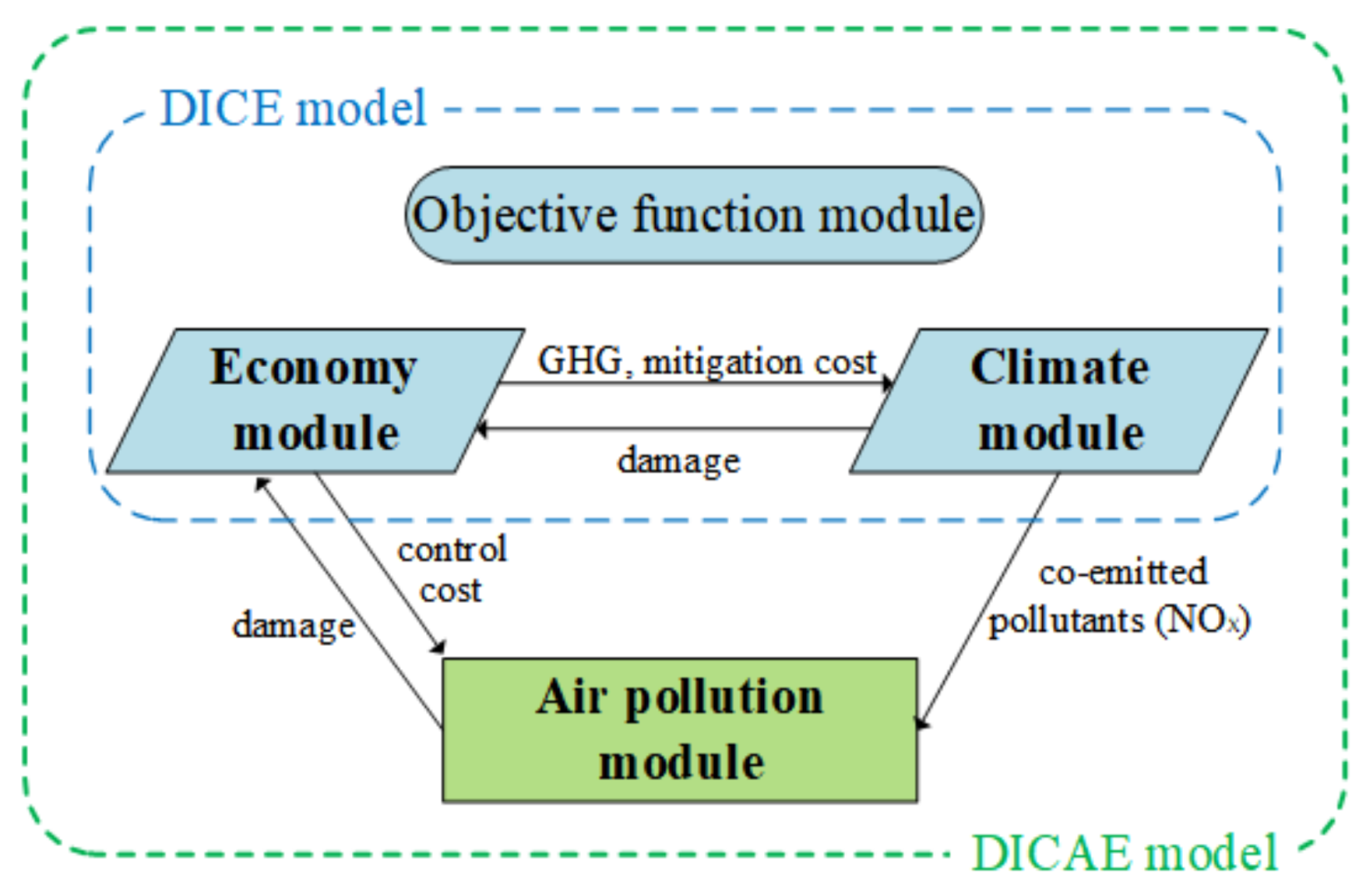
2.1. The DICAE Model

The DICE model consists of three modules: objective function module, global economic module and the climate change module [22]. Through the monetization of climate change damages and mitigation costs, the climate module is linked to the economic module, then the whole model seeks for the optimal economic development and climate mitigation pathway under the goal of social utility maximization.

Our study is based on the DICE-2013R version [23]. The original time step of DICE-2013R is five years, but it takes a long time for the computer to solve the nonlinear optimization problem (NLP), especially when we do Monte Carlo simulations by interfacing General Algebraic Modeling System (GAMS) and MATrix LABoratory (MATLAB) (which will be explained in detail in Section 2.3). As the choice of time step does not affect the model results, this paper sets it to 10-year to improve the computing efficiency. Accordingly, the parameters and initial variables relating to time step need to be adjusted (See

Table A1. The adjusted parameters and initial variables in the Dynamic Integrated model of Climate and the Economy (DICE) model.

Parameter/Variable	Value	Parameter/Variable	Value
Preference		Carbon Cycle
Elasticity of marginal utility of consumption	1	Initial Concentration in atmosphere 2010 (GtC)	830.4
Initial rate of social time preference (per year)	0.03	Initial Concentration in upper strata 2010 (GtC)	1527
Decrease in social time preference (per year)	0.002572	Initial Concentration in lower strata 2010 (GtC)	10,010
Population & Technology		Carbon cycle transition matrix ${\phi }_{11}$	0.912
Initial population growth rate (per decade)	0.08	Carbon cycle transition matrix ${\phi }_{12}$	0.088
Decrease in population growth rate (per decade)	0.3	Carbon cycle transition matrix ${\phi }_{21}$	0.03833
Initial level of total factor productivity	0.032	Carbon cycle transition matrix ${\phi }_{22}$	0.95917
Initial technical progress rate (per decade)	0.15	Carbon cycle transition matrix ${\phi }_{23}$	0.0025
Decrease in technical progress (per decade)	0.005	Carbon cycle transition matrix ${\phi }_{32}$	0.0034
Initial world gross output (trill 2005 USD)	63.69	Carbon cycle transition matrix ${\phi }_{33}$	0.99966
Initial world population (millions)	6838	Climate
Initial capital value (trill 2005 USD)	135	Initial lower stratum temp change (°C from 1900)	0.0068
Depreciation rate on capital (per year)	0.1	Initial atmospheric temp change (°C from 1900)	0.8
Capital elasticity coefficient	0.3	Carbon emissions from land in 2010 (GtCO2 per decade)	9
Emission		Climate sensitivity	1.41
Initial carbon intensity (emission-output rate)	0.12618	Climate equation coefficient for upper level	0.226
Growth rate of carbon intensity (per decade)	-0.15	Transfer coefficient upper to lower stratum	0.44
Decline rate of decarbonization (per period)	0.0065	Transfer coefficient for lower level	0.02
Damage		Reduction cost
Coefficient of damage function	0	Coefficient of reduction cost function	0.03
Exponent of damage function	0.00267	Exponent of reduction cost function	2.15

in Appendix A).

In this paper, the main work about the modeling is designing an air pollution module and realizing the hard-link with the original DICE model (as shown in Figure 1). In the DICAE model, the economy module and the climate module are same as that in the DICE model [23], so we do not introduce them in this paper. Besides, the explanations of the objective function, as well as how to construct the air pollution module and how it connects with other modules are given in the next sections.

2.1.1. The Objective Function

The DICAE model assumes that economic and climate policies should be designed to optimize the flow of consumption over time. It is important to emphasize that consumption should be interpreted as “generalized consumption,” which includes not only traditional market goods and services like food and shelter but also non-market items such as leisure, health status, and environmental services [23,24].

The mathematical representation of this assumption is that policies are chosen to maximize a social utility function. The following equation is the mathematical statement of the objective function:

$$maxU=\frac{{\sum }_{t=1}^{Tmax}{L}^{\ast }\left(t\right)\left[c{\left(t\right)}^{1-\alpha }/\left(1-\alpha \right)\right]}{{\left(1+\rho \right)}^t}$$

(1)

where $U$ is the present value of total social utility; $L^{\ast }\left(t\right)$ is the effective labors/population; $c\left(t\right)$ is the per capita consumption; $\alpha$ and $\rho$ represent the marginal utility elasticity of consumption and pure social time preference, respectively.

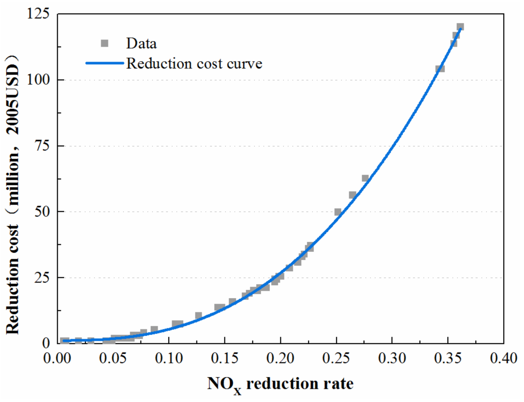
2.1.2. The Air Pollution Module

The air pollution module includes the quantitative description of air pollutant emissions co-emitted with CO₂ emissions, their damages to the socioeconomic system and the costs of abatement. It should be noted that we only analyze one type of air pollutant, NO_X, in this study because of data limitation, and we hope to incorporate more air pollutants, expanding the scope of model applications in future work.

● NO_X emissions

Nitrogen oxides co-emitted with carbon dioxides mainly come from the combustion of coal, oil and natural gas [25], and carbon emissions from energy consumption are also mainly derived from these three major fossil fuels. In this context, we can build the relationship between CO₂ and NO_X based on the homology of emissions.

Assuming that the total energy consumption of the economy is $EC\left(t\right)$, and the proportions of coal, oil and natural gas are $Coal\left(t\right)$, $Oil\left(t\right)$, $Gas\left(t\right)$; The proportion of CO₂ emissions produced by energy consumption is $w$; CO₂ emission factors (emissions from per unit of fuel) of coal, oil and natural gas are $E{F}_{coal}^C$, $E{F}_{oil}^C$, $E{F}_{gas}^C$, and NO_X emission factors are $E{F}_{coal}^N$, $E{F}_{oil}^N$, $E{F}_{gas}^N$; CO₂ emissions and NO_X emissions are $E_C\left(t\right)$ and $E_N\left(t\right)$, respectively. Thus, we can use two equations below to represent the emissions.

$$E_C\left(t\right)\times w=EC\left(t\right)\times \left[Coal\left(t\right)\times E{F}_{coal}^C+Oil\left(t\right)\times E{F}_{oil}^C+Gas\left(t\right)\times E{F}_{gas}^C\right]$$

(2)

$$E_N\left(t\right)=EC\left(t\right)\times \left[Coal\left(t\right)\times E{F}_{coal}^N+Oil\left(t\right)\times E{F}_{oil}^N+Gas\left(t\right)\times E{F}_{gas}^N\right]$$

(3)

Please note that the NO_X emissions calculated in Equation (2) are only the emissions from fossil fuel combustion, under the assumption that all the NO_X co-emitted with CO₂ comes from the combustion of coal, oil and natural gas. According to Equations (2) and (3), we can get another equation to express NO_X emissions:

$$E_N\left(t\right)=E_C\left(t\right)\times w\times \frac{Coal\left(t\right)\times E{F}_{coal}^N+Oil\left(t\right)\times E{F}_{oil}^N+Gas\left(t\right)\times E{F}_{gas}^N}{Coal\left(t\right)\times E{F}_{coal}^C+Oil\left(t\right)\times E{F}_{oil}^C+Gas\left(t\right)\times E{F}_{gas}^C}$$

(4)

Then we use ${\alpha }_{CN}$ to indicate the amount of NO_X emissions co-emitted by a unit of CO₂ emission, calling it co-emit coefficient.

$${\alpha }_{CN}=w\times \frac{Coal\left(t\right)\times E{F}_{coal}^N+Oil\left(t\right)\times E{F}_{oil}^N+Gas\left(t\right)\times E{F}_{gas}^N}{Coal\left(t\right)\times E{F}_{coal}^C+Oil\left(t\right)\times E{F}_{oil}^C+Gas\left(t\right)\times E{F}_{gas}^C}$$

(5)

$$E_N\left(t\right)=E_C\left(t\right){\alpha }_{CN}$$

(6)

Based on the above equations, it is possible to calculate the NO_X emissions based on the CO₂ emissions and the energy consumption structure. In addition, if there are actions to reduce CO₂ and NO_X, Equation (6) needs to be modified. Here we use ${\mu }_C\left(t\right)$ and ${\mu }_N\left(t\right)$ to indicate the emission reduction rates of CO₂ and NO_X, respectively, so now their relation satisfies the following equation.

$$E_N\left(t\right)=\left[1-{\mu }_C\left(t\right)\right]\times \left[1-{\mu }_N\left(t\right)\right]\times E_C\left(t\right){\alpha }_{CN}$$

(7)

The emission factors in this paper are collected from IPCC EFDB (Emission Factor Database) [26], and their values are shown in

Table 1. The values of emission factors.

Emission Factor	$\mathit{E}{\mathit{F}}_{\mathit{c}\mathit{o}\mathit{a}\mathit{l}}^{\mathit{C}}$	$\mathit{E}{\mathit{F}}_{\mathit{o}\mathit{i}\mathit{l}}^{\mathit{C}}$	$\mathit{E}{\mathit{F}}_{\mathit{g}\mathit{a}\mathit{s}}^{\mathit{C}}$	$\mathit{E}{\mathit{F}}_{\mathit{c}\mathit{o}\mathit{a}\mathit{l}}^{\mathit{N}}$	$\mathit{E}{\mathit{F}}_{\mathit{o}\mathit{i}\mathit{l}}^{\mathit{N}}$	$\mathit{E}{\mathit{F}}_{\mathit{g}\mathit{a}\mathit{s}}^{\mathit{N}}$
Value (KG/TJ)	94,600	73,300	56,100	300	200	150

.

According to the IPCC AR4 report, CO₂ emissions produced by fossil fuels account for more than 80% of the total anthropogenic CO₂ emissions. Therefore, we set the parameter $w$ as 0.8.

This study assumes that the changes of the energy consumption structure are exogenous. Considering the time span and fitting effect of the energy structure data, we choose the data from the baseline scenario of the Emissions Prediction and Policy Analysis (EPPA) model developed by Massachusetts Institute of Technology (MIT) [27], and get the proportion trends of fossil fuels in the energy consumption structure through the Curve Fitting Toolbox in MATLAB [28] (the coefficient of determination R-square is over 95%). The precise expressions are shown below:

$$Coal\left(t\right)=b_1{t}^2+b_{2}t+b_3$$

(8)

$$Oil\left(t\right)=c_1{t}^{c_2}$$

(9)

$$Gas\left(t\right)=d_{1}t+d_2$$

(10)

The coefficients in the above equations are obtained from data fitting, and their values are shown in

Table 2. The values of coefficients in energy structure equations.

Coefficient	${\mathit{b}}_1$	${\mathit{b}}_2$	${\mathit{b}}_3$	${\mathit{c}}_1$	${\mathit{c}}_2$	${\mathit{d}}_1$	${\mathit{d}}_2$
Value	−0.000225	0.01245	0.2438	0.4058	−0.082	−0.0027	0.218

.

● NO_X damages

Inspired by the DICE model, which divides the impacts of carbon dioxide on the socio-economic system into two parts—environmental damages caused by emissions and control costs of mitigation measures, we divide the impacts of NO_X into damages and costs in the DICAE model. As for damages of air pollutants, many studies have approximated them as human health losses. For example, Yang et al. represented the environmental damages of SO₂, NO_X and PM₁₀ by the value of premature deaths [29]. Thus, in this paper, we also indirectly quantify the environmental damages of NO_X emissions through health impairment. Meanwhile, in terms of abatement costs, this paper fits a cost curve of NO_X abatement, which will be described in detail in the next sub-section.

To evaluate the health impacts caused by NO_X, the inhalation factor method inferred by Li was adopted [30]. Inhalation factor refers to the proportion of total pollutants absorbed by the human body, so it is a dimensionless parameter and can also be called exposure efficiency [31]. This method calculates the inhaled dose in human body firstly, then calculates the health impacts through a dose-response coefficient, and it can be used to evaluate the economic losses further.

The formula for calculating the health damages of NO_X is as follows:

$$HE=\gamma \times IF\times E_N\left(t\right)$$

(11)

where $HE$ is the health losses (incidence and mortality); $\gamma$ is the coefficient of dose-response, which represents the health impacts caused by per unit of inhaled NO_X; The inhalation factor is $IF$, and the value is 2.47 × 10⁻⁶ [32]; $E_N\left(t\right)$ indicates the NO_X emissions which we have discussed in the previous section.

● NO_X reduction costs

In this paper, the reduction costs are calculated based on the NO_X emission data in the RAINS model developed by IIASA [33]. Figure 2 shows the NO_X reduction cost curve, and the corresponding function of the curve is:

$$T{C}_N\left(t\right)={\theta }_3+{\theta }_4\times {\left[{\mu }_N\left(t\right)\right]}^{{\theta }_5}$$

(12)

where ${\theta }_3=1.280$, ${\theta }_4=1643.047$, ${\theta }_5=2.584$; ${\mu }_N\left(t\right)$ refers to the reduction rate of NO_X, and $T{C}_N\left(t\right)$ refers to the reduction costs.

2.1.3. Linking with the DICE Model

After creating the air pollution module, we can extend the DICE model into the DICAE model. As shown in Figure 1, carbon emissions in the climate module connect with NO_X emissions in the air pollution module, which has already been realized through Equation (7). And environmental damages and reduction costs of air pollutants would influence the final output in the economic module through the following Equations (13)–(18).

In the original economic module, the production function is based on a Cobb-Douglas function which is fixed-scale returns, and then we introduce a climate-feedback coefficient to form an expression of the aggregate output:

$$Y\left(t\right)=\phi \left(t\right)A\left(t\right)K{\left(t\right)}^{\delta }L{\left(t\right)}^{1-\delta }$$

(13)

where $Y\left(t\right)$ is the total economic output at time $t$; $A\left(t\right)$, $K\left(t\right)$ and $L\left(t\right)$ represent the total factor productivity, capital stock and labors (population) at time $t$; $\delta$ represents the capital elasticity; $\phi \left(t\right)$ is the climate-feedback coefficient which is calculated by environmental damages $DA\left(t\right)$ and mitigation costs $TC\left(t\right)$ of CO₂, and its specific expression is:

$$\phi \left(t\right)=\frac{1-TC\left(t\right)}{1+DA\left(t\right)}$$

(14)

After introducing the air pollution module, we update the above equations:

$$Y^{\ast }\left(t\right)={\phi }^{\ast }\left(t\right)A^{\ast }\left(t\right)K{\left(t\right)}^{\delta }{L}^{\ast }{\left(t\right)}^{1-\delta }$$

(15)

$${\phi }^{\ast }\left(t\right)=\frac{1-T{C}_C\left(t\right)-T{C}_N\left(t\right)}{1+DA\left(t\right)}$$

(16)

$$L^{\ast }\left(t\right)=L\left(t\right)\times \left[1-\mathsf{\omega }\left(t\right)\right]$$

(17)

$$A^{\ast }\left(t\right)=A\left(t\right)\times \left[1-v\left(t\right)\right]$$

(18)

By adding NO_X reduction costs $T{C}_N\left(t\right)$, Equation (16) adjusts the climate-feedback coefficient into a climate & environment-feedback coefficient ${\phi }^{\ast }\left(t\right)$. Then this paper reflects the health damages of NO_X on the population and productivity. Concretely, the mortality rate $\mathsf{\omega }\left(t\right)$ would affect the effective labors $L^{\ast }\left(t\right)$, while the incidence rate $v\left(t\right))$ could reduce the actual productivity $A^{\ast }\left(t\right)$.

Consequently, the two-way feedback between the air pollution module and the original DICE model is realized in the DICAE model. The DICAE model totally includes 45 parameters and 29 variables, since the number of equations is greater than the number of variables, the optimal solution for each variable can be obtained. We solve this NLP problem using the GAMS software [34].

2.2. Scenarios

To discuss the influence of adding NO_X on the model results and compare the implementation effects of CO₂ reduction policies, as well as NO_X control policies with different intensity levels, setting different scenarios for future emission target is extremely necessary. Therefore, seven mixed emission scenarios are developed in this paper to compare the effects of different emission reduction policies for CO₂ and NO_X. These scenarios are made up of three CO₂ emission scenarios: reference scenario (REF), mitigation scenarios (MIT550 and MIT450), and three NO_X emission scenarios: no policy (NP), relaxed policy (RP), and stringent policy (SP). The specific meanings of each scenario are listed in

Table 3. Overview of emission scenarios in the DICAE model.

Scenario	CO2 Emission Policy	NOX Emission Policy
REF-NP	No policy	No policy
MIT550-NP	Achieve 550 ppm stabilization	No policy
MIT550-RP	Achieve 550 ppm stabilization	Reduction rate is 20%
MIT550-SP	Achieve 550 ppm stabilization	Reduction rate is 60%
MIT450-NP	Achieve 450 ppm stabilization	No policy
MIT450-RP	Achieve 450 ppm stabilization	Reduction rate is 20%
MIT450-SP	Achieve 450 ppm stabilization	Reduction rate is 60%

.

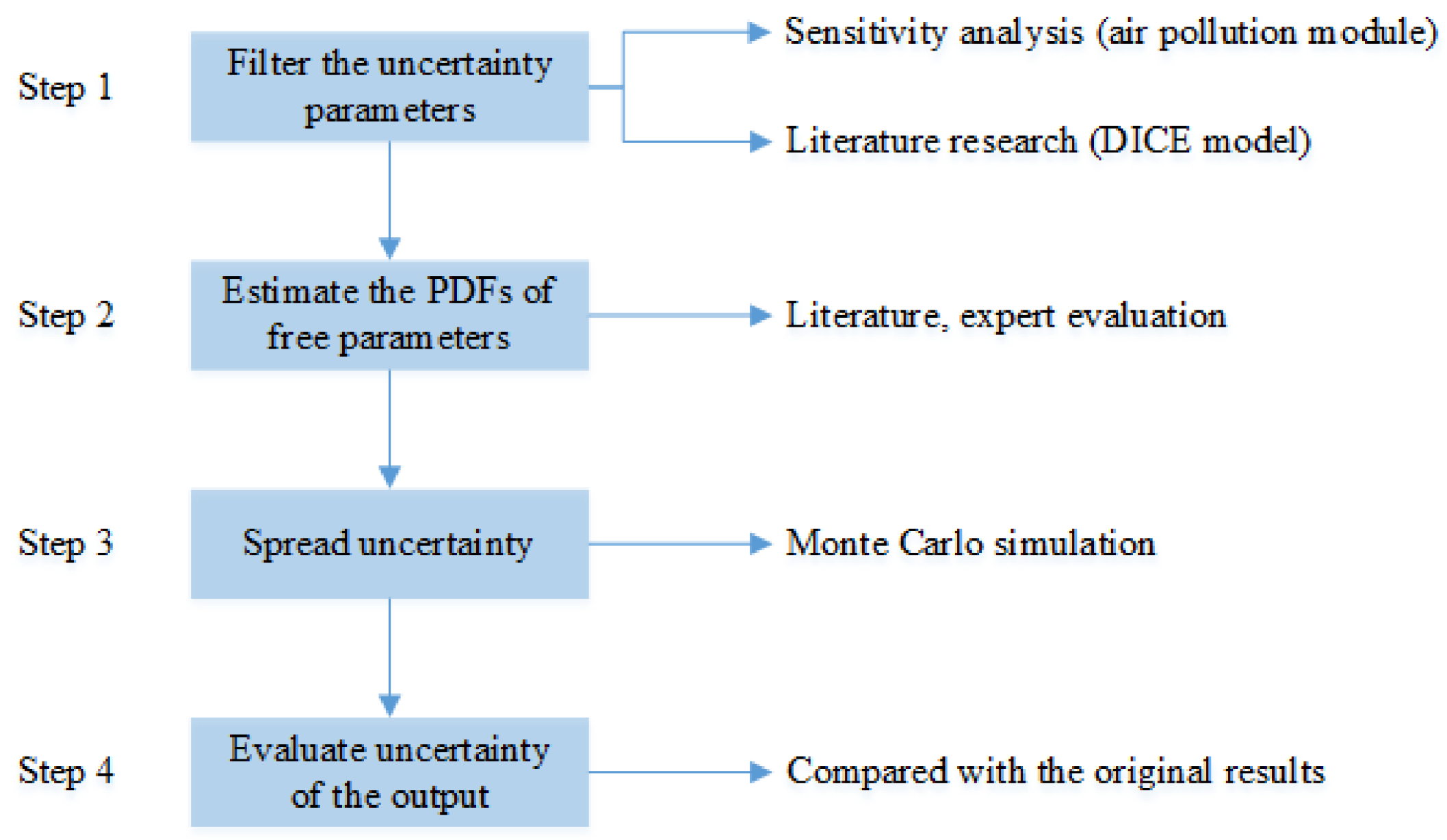
2.3. Uncertainty Analysis

In the DICAE model, in addition to the deviation of the model assumptions from the scientific facts, some parameters are collected from expert evaluation or data fitting, which also contains a certain degree of subjectivity and bias. In this case, it is worth doing uncertainty analysis of free parameters.

The framework of uncertainty analysis is shown in Figure 3. Since the DICAE model consists of the DICE model and an air pollution module, so we filter sensitive parameters from these two parts, respectively. First, we filter the sensitive parameters of the air pollution module by single-value sensitivity analysis, and then identify the parameters which have relatively great impacts on model outputs in the climate module and the economy module based on the previous literature [35,36,37,38]. After defining the probability density functions (PDFs) of these selected free parameters, Monte Carlo simulation is applied to spread the joint uncertainties of all the sensitive parameters through interfacing GAMS and MATLAB software [39]. Finally, we compare the new outputs with the original results. Figure 3 shows the framework of uncertainty analysis.

3. Results

This section reports the model results under different emission scenarios to answer the four sub-questions proposed in the introduction section. Hence, the results are presented in four sections: (1) co-benefits for NO_X emission reduction across scenarios; (2) predicted climate change across scenarios; (3) effects of joint policies for CO₂ and NO_X emission reduction, and; (4) results of the uncertainty analysis.

3.1. Co-Benefits for NO_X Emission Reduction

In this section, we quantify the co-benefits of climate mitigation for NO_X abatement and compare the co-benefits under different policy scenarios. We unify NO_X emissions into the no policy scenario (NP) and divide CO₂ emissions into three scenarios of different policy intensity (REF, MIT550 and MIT450), so that we can discuss the co-benefits under three combined scenarios (REF-NP, MIT550-NP and MIT450-NP).

Figure 4 and Figure 5 illustrate that climate mitigation can effectively reduce carbon dioxide emissions and significantly reduce nitrogen dioxides emissions, realizing coordinated emission reduction of both greenhouse gases and air pollutants. In Figure 6, if we do not take any mitigation actions, the CO₂ emission shows an increase tendency, reaching 157.48 Gt in 2050 and nearly 250 Gt in 2150. If the mitigation target is set at 550 × 10⁻⁶CO₂e, the CO₂ emissions will still increase slightly at the initial stage but decline thereafter, and finally become stable after realizing the mitigation target. When the target is set to be more ambitious, at 450 × 10⁻⁶ CO₂e, the emissions decline rapidly in the early periods, and gradually be stabilized at around 10 Gt. As for NO_X (Figure 5), the changes of NO_X emissions are largely the same as CO₂. In the absence of carbon mitigation, a great amount of CO₂ emissions will co-emit lots of NO_X, and the quantity can be 0.6 Gt/year. Fortunately, reducing CO₂ emissions can at least cut down 15% of the NO_X emissions in the first two periods. Comparing MIT550-NP and MIT450-NP, it is not difficult to find that the more severe the climate mitigation target, the more obvious co-benefits for NO_X abatement. However, finally, NO_X emissions can be stabilized at a low level in both cases.

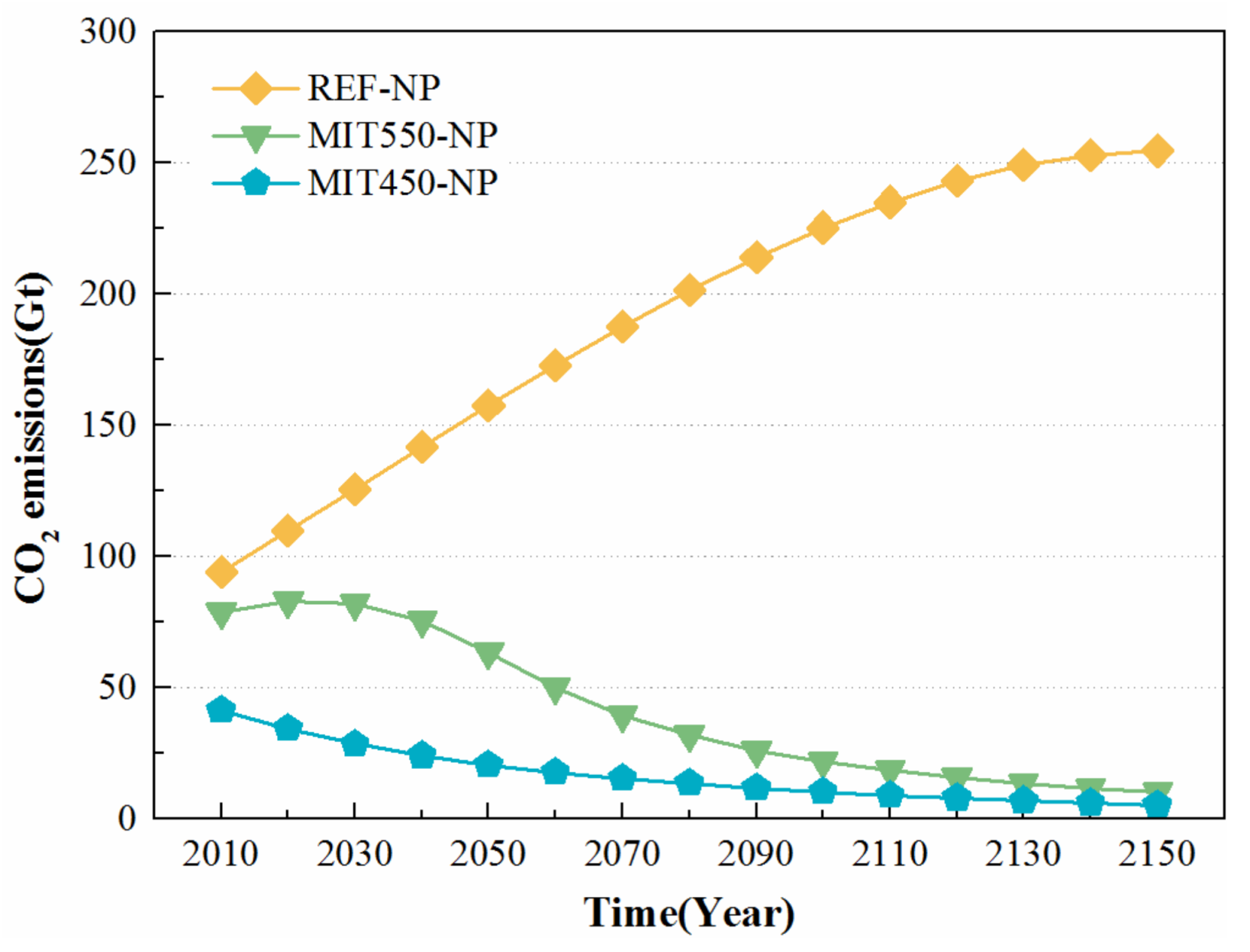
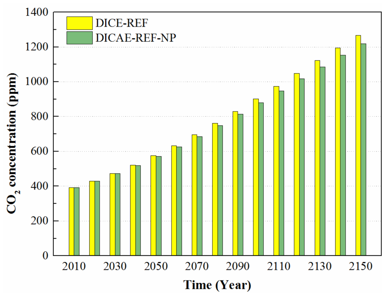
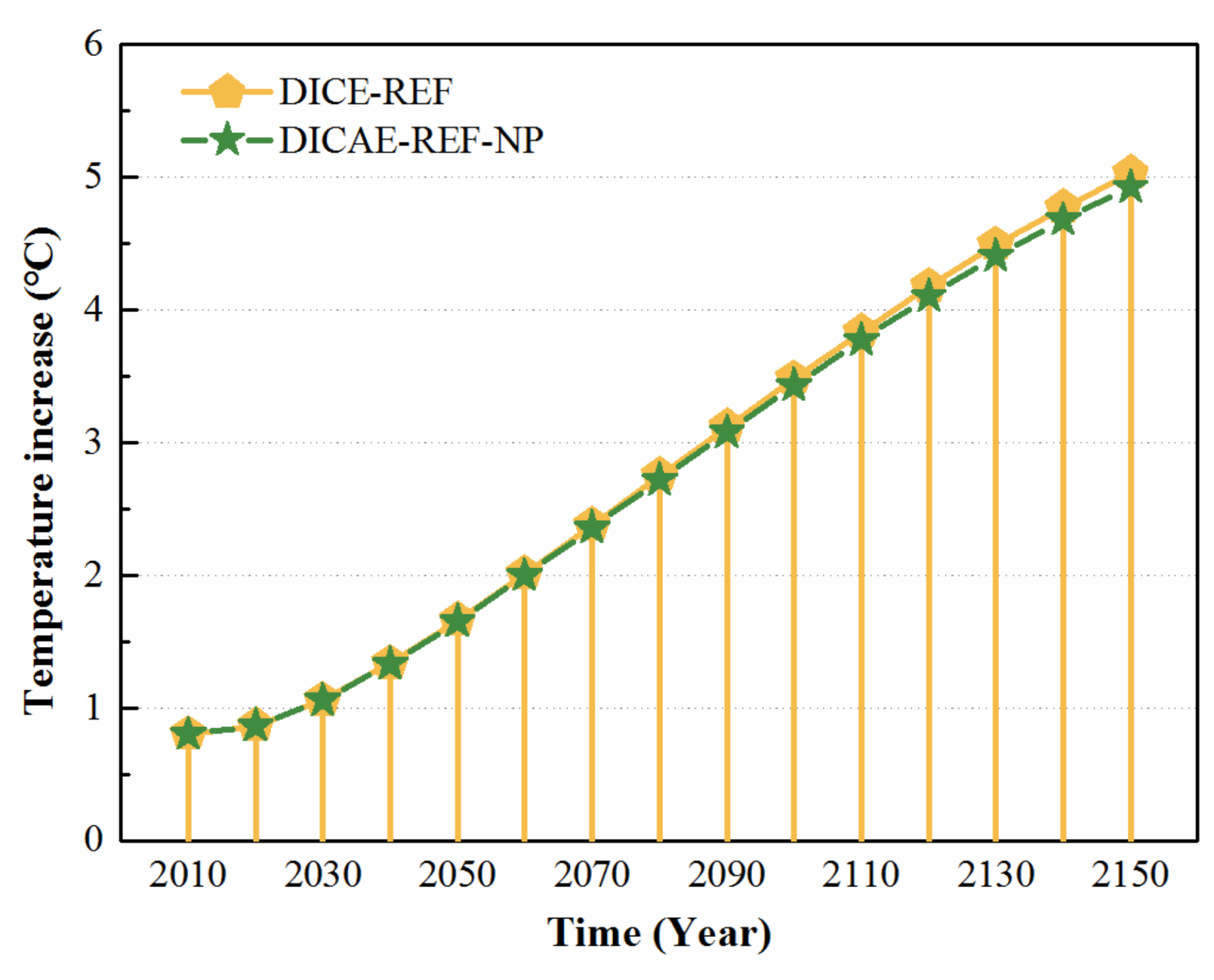
3.2. Climate Change Prediction

To answer question 2 raised in the introduction section, we compare the CO₂ concentration and global temperature increase of the reference scenario in DICE model (not listed in Table 3, this scenario means no climate mitigation in DICE model) and the REF-NP scenario in DICAE model.

From Figure 6, we can find that in the first three periods, the atmospheric CO₂ concentration after considering NO_X (DICAE-REF-NP scenario) is basically the same as it does when NO_X is not considered (DICE-REF scenario). But later, the concentration in the DICAE model is lower than that in the DICE, and the gap is gradually increasing. Correspondingly, the global temperature rise in the DICAE-REF-NP scenario is also progressively lower than that in the DICE-REF scenario over time (indicated in Figure 7). By 2150, the difference reaches approximately 0.103 °C.

After considering the co-emitted NO_X from CO₂, per unit CO₂ emissions will bring greater losses to the whole economy, as it includes damages from both carbon dioxide and nitrogen dioxides. With the increase of CO₂ emissions from human activities, it can produce more co-emitted air pollutants, then, the negative impacts on the economic output becomes increasingly severe. Therefore, under the goal of maximizing the discounted sum of the utilities of per capita consumption in the DICAE model, less anthropogenic CO₂ would be emitted as considering the co-benefits of CO₂ mitigation, even in the no mitigation policy scenario (DICAE-REF-NP). As a result, less CO₂ is emitted in DICAE-REF-NP, which leads to lower concentration and lower temperature rise in the middle and later periods.

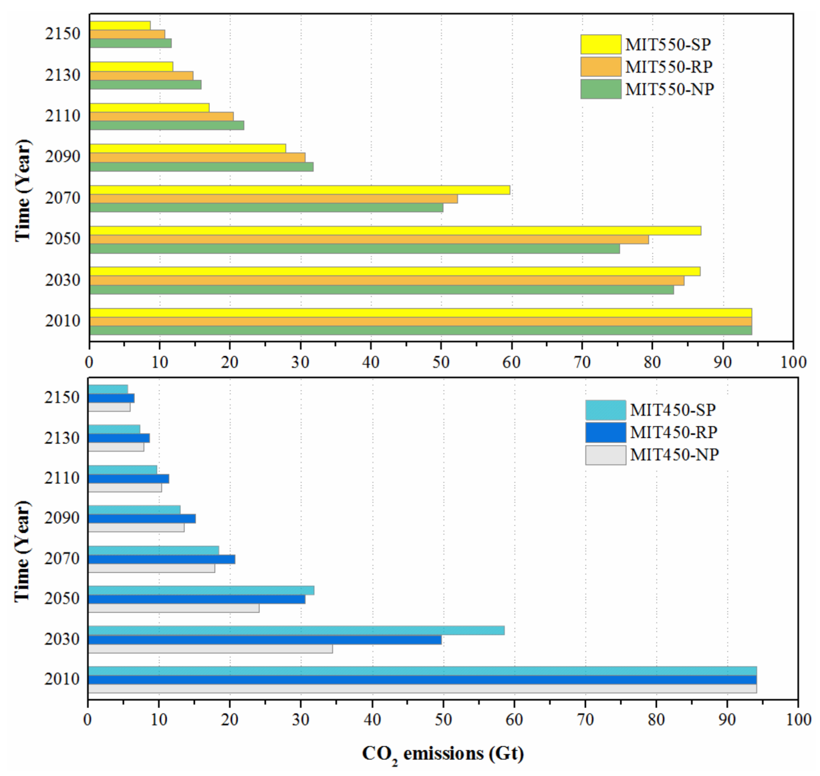
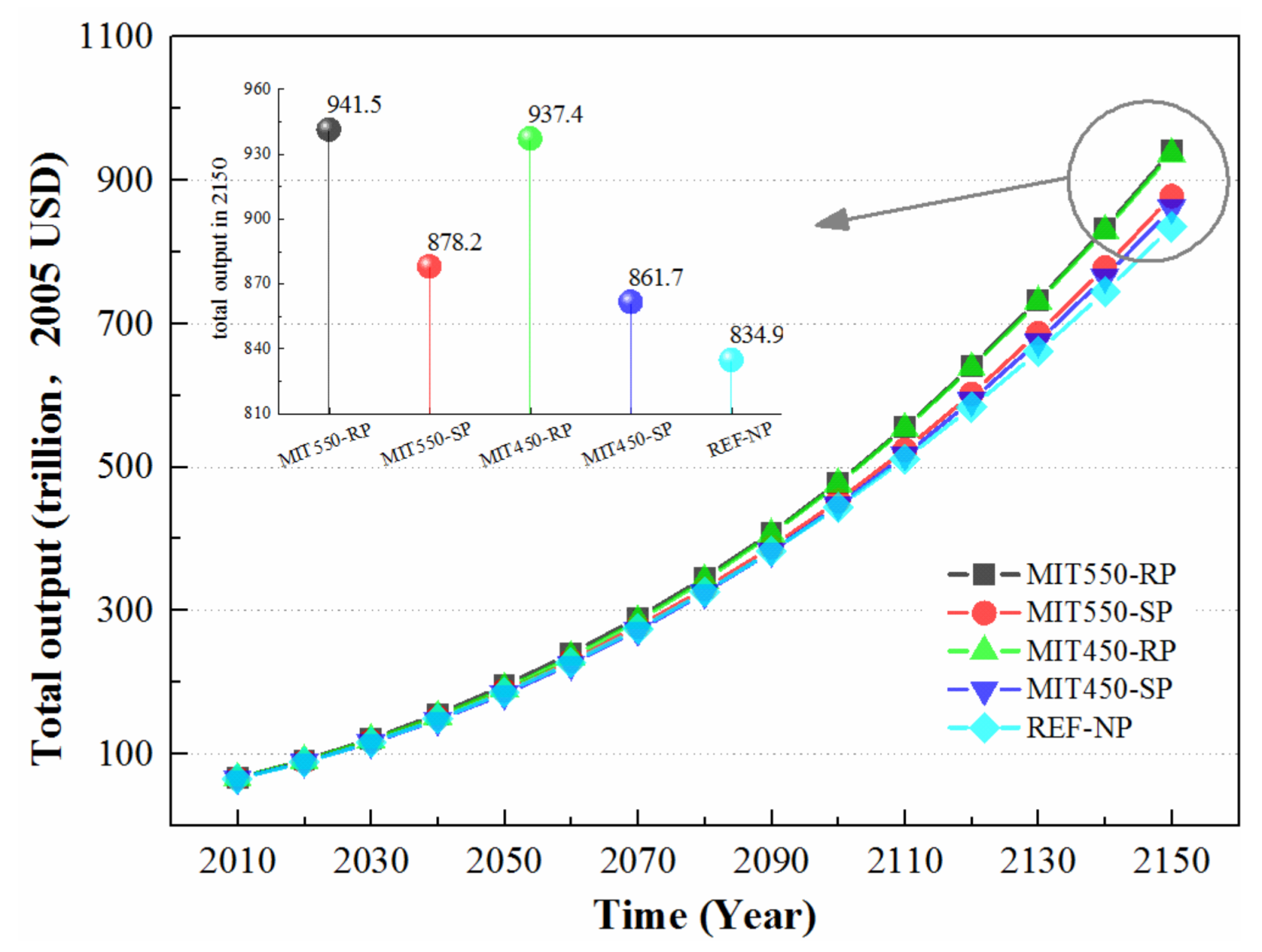
3.3. Effects of Joint Policies

Since climate mitigation can bring co-benefits for air pollutant management, in turn, will air pollution policies affect CO₂ emissions? Figure 8 states the answer. Since NO_X emissions associated with CO₂ emissions from combusting fossil fuels can be reduced through end-of-pipe technology, some of them will not emit into the atmosphere, so the environmental damages can be decreased, which means the negative impact of per unit CO₂ emission can be weakened. Hence, the amount of CO₂ emissions in the early periods is larger than that under the no NO_X policy scenario. When we compare MIT550-SP with MIT550-RP or MIT450-SP with MIT450-RP, it reveals that stricter NO_X reduction policies will allow for more CO₂ emissions. Nevertheless, this situation will change later (after about 2070), because for the aim of achieving the climate goal, CO₂ emissions must be drastically reduced at that time, which can compensate for the previous over-emissions. Now the more severe NO_X reduction policy corresponds to a lower level of CO₂ emissions, although the gaps among different scenarios are not obvious. In this case, in terms of CO₂ emissions, there is no evidence to prove that the end-of-pipe technology for NO_X will have absolute positive or negative synergies on CO₂ mitigation, because the short-term impacts are different from that in the long term.

Now we explore the impacts of joint policies on world economic output and social utility From Figure 9, we can see that the total outputs in different scenarios all have an increase trend, and the gaps are totally negligible in the early periods but become bigger in the later periods. For ease of comparison, the total output in 2150 is enlarged to the upper left corner of Figure 9, so it is easy to find that the outputs from high to low are: MIT550-RP > MIT450-RP > MIT550-SP > MIT450-SP > REF-NP. It suggests that no emission reduction actions or radical reduction measures cannot bring the highest economic output, while the relatively moderate emission reduction policies for CO₂ and NO_X can produce the greatest economic benefits. The reason behind this phenomenon is clear. Without mitigation, the environmental damages of CO₂ and NO_X will affect the economic growth, but if people make ambitious efforts to reduce CO₂ emissions, they need to invest a lot, which may reduce the net economic output and affect economic growth when the co-benefits cannot cover the mitigation costs. For instance, in the MIT450-RP scenario, people need to invest 8 trillion USD/year more for mitigation than that in the MIT550-RP scenario, which can produce more co-benefits for NO_X emission reduction. However, the overall economic output would reduce by 0.43% in MIT450-RP even if the co-benefits of mitigation have been added. In contrast, modest joint policies can balance the environmental damages caused by emissions and the fiscal costs of emission reductions, and ultimately maximize the total output.

Comparing the social utilities (the mathematical statement is shown in Equation (1)) in each scenario, as shown in

Table 4. Social utility in different scenarios.

Scenario	Social Utility (Rank)	Scenario	Social Utility (Rank)
REF-NP	6587.163 (5)	MIT450-NP	6436.893 (7)
MIT550-NP	6546.670 (6)	MIT450-RP	6580.858 (4)
MIT550-RP	6639.827 (3)	MIT450-SP	6690.395 (2)
MIT550-SP	6731.567 (1)

, the quantities from high to low are: MIT550-SP > MIT450-SP > MIT550-RP > MIT450-RP > REF-NP > MIT550-NP > MIT450-NP. It illustrates that the combination of a modest CO₂ policy and a stringent NO_X policy yields the greatest utility and other joint policies can also make higher social utilities than the no policy scenario (REF-NP). It is worth noting that the social utility in the case of only reducing CO₂ emissions but without NO_X abatement (MIT550-NP) would be even lower than the REF-NP scenario. On the one hand, the costs of carbon mitigation cause a burden on the economy which does harm to the utility growth. On the other hand, it shows that the co-benefits of CO₂ reduction on NO_X abatement is not enough to cover the negative externalities caused by air pollutants. Therefore, the end-of-pipe technology for NO_X is still quite necessary.

3.4. Uncertainties

The single-value sensitivity analysis is carried out by floating $\pm 5\%$ on the free parameters in air pollution module. According to the fluctuation of model outputs, we select three sensitive parameters: coal consumption coefficient 2, NO_X reduction cost coefficient 1, and the proportion of CO₂ emissions from energy consumption. What’s more, their induced fluctuations of the model outputs are all in the range of 1%~2%, which means the newly extended air pollution module doesn’t introduce much uncertainty. As for the other three modules, we select nine sensitive parameters and define their probability distribution functions (PDFs) based on some previous studies pertaining to uncertainty analysis of the DICE model [35,36], including some researches discussing fat-tailed probability distributions and unbounded climate risks [37,38]. Therefore, we filter 12 sensitive parameters in the DICAE model, and their PDFs are listed in

Table 5. Probability distribution of free parameters.

No.	Free Parameter	PDF	Parameters of the PDF
01	Capital elasticity coefficient	Beta distribution	up = 0.4, lo = 0.2, $\mu$ = $\nu$ = 9
02	Capital depreciation rate	Beta distribution	up = 0.12, lo = 0.08, $\mu$ = $\nu$ = 4.5
03	Initial productivity growth rate	Beta distribution	up = 0.19, lo = 0.11, $\mu$ = $\nu$ = 4.5
04	Decline rate of population growth	Beta distribution	up = 0.4, lo = 0.2, $\mu$ = $\nu$ = 6
05	Pure rate of social time preference	Beta distribution	up = 0.06, lo = 0, $\mu$ = 7,$\nu$ = 4
06	Growth rate of carbon intensity	Beta distribution	up = −0.05, lo = −0.2, $\mu$ = 4, $\nu$ = 6
07	Carbon reduction cost coefficient 1	Beta distribution	up = 0.04, lo = 0.02, $\mu$ = $\nu$ = 5.5
08	Climate sensitivity	Logarithmic normal distribution	avg = 1.071, sd = 0.527
09	Damage function exponent	Triangular distribution	max = 5, min = 1, avg = 2
10	Coal consumption coefficient 2	Normal distribution	avg = 0.012, sd = 1
11	NOX reduction cost coefficient 1	Normal distribution	avg = 1643.048, sd = 0.527
12	Proportion of CO2 emissions from energy consumption	Normal distribution	avg = 0.8, sd = 1

Note: $\mu$ and $\nu$ are two parameters of the beta distribution function, which can control the distribution shape; up = upper limit, lo = lower limit, avg = average value, sd = standard deviation, max = maximum, min = minimum. Probability distribution functions (PDFs).

.

Then, according to the PDFs, we adopt the Monte Carlo simulation to spread the uncertainties of 12 free parameters and focus on three indicate endogenous variables (temperature increase, co-emitted NO_X and total output) from different modules to check the changes of model results. After perturbing these free parameters randomly by ±5% through 1000 simulations, the distributions of the indicator variables in the MIT550-RP scenario in year 2050 are shown in Figure 10. Their values can pass the normal distribution test. Based on the 3σ principle, the 95% confidence intervals for each indicator variable can be calculated using the mean value and standard deviation. Choosing 2050 as an example, the confidence interval of temperature increase is (1.432, 1.628) °C, and the interval for NO_X emissions is (0.082, 0.120) Gt, as for total output, it is (182.898, 194.439) trillion USD.

Similarly, the confidence intervals in each year can be estimated. Figure 11 depicts the original results of the indicator variables from 2010 to 2150, as well as their 95% confidence intervals from Monte Carlo simulation. It can be found that after introducing the randomness of free parameters, the model results would have a great deal of uncertainties. First, for temperature increase, uncertainties in the later periods are obvious, since the uncertainties gradually accumulate, leading to great deviations from the original output. Moreover, the blue line is a bit below the center of the light blue shade, indicating that the mean value of temperature increase in the uncertain condition is higher than that of the original model. It may relate to our definition about the PDF of the climate sensitivity parameter based on the fat-tailed distribution. Second, in view of NO_X emissions co-emitted with CO₂ emissions, the values fluctuate within the ±20% range of the original result, which means when all the 12 sensitive parameters in the DICAE model are perturbed randomly by ±5%, it may be difficult to get an accurate estimation of NO_X emissions. Finally, as for economic output, the initial confidence interval is (65.47, 67.58) trillion USD, with a fluctuation range of 3.15%, but the interval becomes larger afterwards. In 2150, the interval is (828.54, 1011.54) trillion USD, and the fluctuation range is 20.18%. Likewise, it demonstrates that the uncertainty in subsequent periods of the model is larger than that in the early years. Although there are lots of uncertainties, if we understand the sources and scope of the uncertainty, the model results can still have reasonable applications.

4. Conclusions

Integrated Assessment Models (IAM) that do not consider co-benefits would inevitably underestimate the real benefits of climate mitigation actions and may hamper policy makers from selecting the optimal mitigation pathways. In this paper, we extend the Dynamic Integrated model of Climate and the Economy (DICE) model into the Dynamic Integrated model of Climate, Air pollution and the Economy (DICAE) model by linking an air pollution module, and taking NO_X as an example, the co-benefits of CO₂ mitigation for air pollutants reduction are analyzed. Furthermore, the predicted climate change, the economic output and social utility of joint policies are also explored. At last, we do an uncertainty analysis to test the robustness of the DICAE model and give the uncertainty ranges of model results. The following implications can be drawn from this study.

Firstly, CO₂ mitigation has significant co-benefits for NO_X emission reduction, which can reduce at least 15% of the NO_X emissions, and the emission reduction rate would be greater if we increase the climate mitigation intensity. These benefits can invariably occur in the short-term and lower the net costs of climate mitigation. However, the end-of-pipe technology for NO_X emissions is also necessary, as it will not be cost-effective when NO_X emission reduction is achieved completely depending on ambitious CO₂ mitigation. The predominant joint policy is the one that can coordinate the environmental damages and mitigation costs, maximizing the total output or social utility in a sustainable pathway. The single-value sensitivity analysis identifies three sensitive parameters from the air pollution module. After disturbing them by ±5%, respectively, the changes of main output variables are negligible, which means that the new module doesn’t introduce many uncertainties. Further, the results of Monte Carlo simulation of 12 selected sensitive parameters manifest that the uncertainties in the later period of the model are larger than that in the early years. Ignoring these uncertainties may cause great risks.

Secondly, there are some implications for policy decision. Comparing the climate change predictions in the DICE model and the DICAE model, the global warming would be relieved to some extent in DICAE, because humans tend to take active mitigation actions due to the incentives from co-benefits for NO_X emission reduction. Thus, policy makers should recognize the co-benefits of climate mitigation policies and join in climate actions actively. Especially for developing countries, the government should be aware that, when compared to the long-term and global features of climate mitigation, co-benefits for air pollutants can happen quickly and locally, which would offset some costs of climate policies and strike a balance between short-term interests and long-term development. Furthermore, in the joint policy scenarios, the economic output and social utility are both higher than that in single policy scenarios, which indicate the significance of combining climate policies with air pollution policies and coordinating their intensities to make full use of the co-benefits between them.

Finally, as for modeling work, our study shows the attempt to incorporate co-benefits of climate mitigation into the IAM framework which can capture the feedbacks between the socioeconomic system and the natural system, as well as provide cost-benefit analysis for various policy scenarios. Based on the DICAE model, this paper gives more accurate estimations of these co-benefits for NO_X emission reduction and predicted future climate change after considering the response from human-beings and the natural system in an integrated policy assessment framework. However, it has some limitations and more future work needs to be done. For instance, we can apply the framework of the DICAE model to other air pollutants, getting a more comprehensive analysis about co-benefits for air pollutants. Another promising area of future research is realizing the partitioning of the model, to focus on specific mitigation policies within a country or a region, which could lay a more concrete foundation for informed decision-making.

References

1. Swart, R.; Amann, M.; Raes, F.; Tuinstra, W. A good climate for clean air: Linkages between climate change and air pollution. An editorial essay. Clim. Chang. 2004, 66, 263–269. [Google Scholar] [CrossRef]
2. Wei, W.; Li, P.; Wang, S.; Gao, J. CO2 emission driving forces and corresponding mitigation strategies under low-carbon economy mode: evidence from China’s Beijing-Tianjin-Hebei region. Chin. J. Popul. Resour. Environ. 2017, 15, 109–119. [Google Scholar] [CrossRef]
3. Bollen, J.; Guay, B.; Jamet, S.; Corfee-Morlot, J. Co-Benefits of Climate Change Mitigation Policies: Literature review and New Results; OECD Economics Department Working Papers 693; OECD Publishing: Paris, France, 2009. [Google Scholar]
4. Davis, D.L.; Kjellstrom, T.; Slooff, R.; Mcgartland, A.; Atkinson, D. Short-term improvements in public health from global-climate policies on fossil-fuel combustion: An interim report. Lancet 1997, 350, 1341–1349. [Google Scholar] [CrossRef]
5. Dessus, S.; O’connor, D. Climate policy without tears cge-based ancillary benefits estimates for Chile. Environ. Resour. Econ. 2003, 25, 287–317. [Google Scholar] [CrossRef]
6. Shrestha, R.M.; Pradhan, S. Co-benefits of CO2 emission reduction in a developing country. Energy Policy 2010, 38, 2586–2597. [Google Scholar] [CrossRef]
7. Rypdal, K.; Rive, N.; Astrom, S.; Karvosenoja, N.; Aunan, K. Nordic air quality co-benefits from European post-2012 climate policies. Energy Policy 2007, 35, 6309–6322. [Google Scholar] [CrossRef]
8. Dong, H.; Dai, H.; Liang, D.; Fujita, T.; Geng, Y. Pursuing air pollutant co-benefits of CO2, mitigation in China: A provincial leveled analysis. Appl. Energy 2015, 144, 165–174. [Google Scholar] [CrossRef]
9. Davis, D.L.; Krupnick, A.; Mcglynn, G. Ancillary benefits and costs of greenhouse gas mitigation: An overview. In Ancillary Benefits and Costs of Greenhouse Gas Mitigation; OECD: Paris, France, 2000; pp. 9–50. ISBN 9789264188129 (ebook). 9789264185425 (paperbook). [Google Scholar]
10. National Research Council. Hidden Costs of Energy: Unpriced Consequences of Energy Production and Use; The National Academies Press: Washington, DC, USA, 2010; ISBN 9780309155809 (ebook). 9780309146401 (paperbook). [Google Scholar]
11. Burtraw, D.; Krupnick, A.; Palmer, K.; Paul, A.; Toman, M. Ancillary benefits of reduced air pollution in the US from moderate greenhouse gas mitigation policies in the electricity sector. J. Environ. Econ. Manag. 2003, 45, 650–673. [Google Scholar] [CrossRef]
12. Parson, E.A.; Fisher-Vanden, A.K. Integrated assessment models of global climate change. Annu. Rev. Energy Env. 1997, 22, 589–628. [Google Scholar] [CrossRef]
13. Metcalf, G.E.; Stock, J. The Role of Integrated Assessment Models in Climate Policy: A User’s Guide and Assessment; The Harvard Project on Climate Agreements Discussion Paper; Harvard Kennedy School: Cambridge, MA, USA, 2015; pp. 15–68. [Google Scholar]
14. Weyant, J. Some contributions of integrated assessment models of global climate change. Rev. Environ. Econ. Policy 2017, 11, 115–137. [Google Scholar] [CrossRef]
15. Bollen, J.; Zwaan, B.; Brink, C.; Eerens, H. Local air pollution and global climate change: A combined cost-benefit analysis. Resour. Energy Econ. 2009, 31, 161–181. [Google Scholar] [CrossRef]
16. Wager, F.; Amann, M.; Borken, K.J.; Cofala, J.; Höglund, I.L. Sectoral marginal abatement cost curves: Implications for mitigation pledges and air pollution co-benefits for annex I countries. Sustain. Sci. 2012, 7, 169–184. [Google Scholar] [CrossRef]
17. Rao, S.; Klimont, Z.; Leitao, J.; Riahi, K.; van Dingenen, R. A multi-model assessment of the co-benefits of climate mitigation for global air quality. Environ. Res. Lett. 2016, 11, 124013. [Google Scholar] [CrossRef]
18. Nemet, G.F.; Holloway, T.; Meier, P. Implications of incorporating air-quality co-benefits into climate change policymaking. Environ. Res. Lett. 2010, 5, 014007. [Google Scholar] [CrossRef]
19. Amann, M. Future challenges for integrated assessment modelling. In Proceedings of the Air Pollution and its Relationship to Climate Change and Sustainable Development—Linking Immediate Needs with Long Term Challenges, Gothenburg, Sweden, 12–14 March 2007; Volume 3, pp. 12–14. [Google Scholar]
20. Nordhaus, W.D. An optimal transition path for controlling greenhouse gases. Science 1992, 258, 1315–1319. [Google Scholar] [CrossRef] [PubMed]
21. Zhang, S.H. Co-Benefit Analysis Based on the DICE model. Bachelor’s Thesis, Tsinghua University, Beijing, China, 2015. (In Chinese). [Google Scholar]
22. Nordhaus, W.D. The ‘DICE’ Model: Background and Structure of a Dynamic Integrated Climate-Economy Model of the Economics of Global Warming; Cowles Foundation Discussion Papers 1009; Cowles Foundation for Research in Economics; Yale University: New Haven, CT, USA, 1992. [Google Scholar]
23. Nordhaus, W.D.; Paul, S. DICE 2013R: Introduction and User’s Manual. Available online: http://sites.google.com/site/williamdnordhaus/dice-rice (accessed on 7 April 2018).
24. Nordhaus, W.D. Rolling the ‘DICE’: An optimal transition path for controlling greenhouse gases. Resour. Energy Econ. 1993, 15, 27–50. [Google Scholar] [CrossRef]
25. Qin, X.L. Co-Benefit Analysis of Greenhouse Gas Reduction and Air Pollution Control—A Case Study in Shenzhen. Master’s Thesis, South China University of Technology, Guangzhou, China, 2012. (In Chinese). [Google Scholar]
26. IPCC NGGIP. Emission Factor Database. Available online: http://www.ipcc-nggip.iges.or.jp/EFDB/main.php (accessed on 26 February 2018).
27. Paltsev, S.; Reilly, J.M.; Jacoby, H.D.; Eckaus, R.S.; McFarland, J.R. The MIT Emissions Prediction and Policy Analysis (EPPA) Model: Version 4; MIT Joint Program on the Science and Policy of Global Change: Cambridge, MA, USA, 2005. [Google Scholar]
28. MathWorks. Fit curves and surfaces to data using regression, interpolation, and smoothing. Available online: https://www.mathworks.com/products/curvefitting.html (accessed on 25 March 2018).
29. Yang, X.; Teng, F.; Wang, G. Incorporating environmental co-benefits into climate policies: A regional study of the cement industry in China. Appl. Energy 2013, 112, 1446–1453. [Google Scholar] [CrossRef]
30. Li, J. Valuation of Regional Environmental Damage Cost from Air Pollution. Ph.D. Thesis, Tsinghua University, Beijing, China, 2002. (In Chinese). [Google Scholar]
31. Levy, J.I.; Spengler, J.D.; Hlinka, D.; Sullivan, D.; Moon, D. Using CALPUFF to evaluate the impacts of power plant emissions in Illinois: Model sensitivity and implications. Atmos. Environ. 2002, 36, 1063–1075. [Google Scholar] [CrossRef]
32. Li, J.; Hao, J.; Ye, X.; Zhu, T. Population exposure to air pollutant emissions in Hunan Province. Environ. Sci. 2003, 24, 16–20. [Google Scholar] [CrossRef]
33. Cofala, J.; Syri, S. Nitrogen Oxides Emissions, Abatement Technologies and Related Costs for Europe in the RAINS Model Database; IIASA Interim Report; IIASA: Laxenburg, Austria, 1998. [Google Scholar]
34. Rosenthal, R.E. GAMS: A User’s Guide; GAMS Development Corporation: Washington, DC, USA, 2008. [Google Scholar]
35. Pizer, W.A. The optimal choice of climate change policy in the presence of uncertainty. Resour. Energy Econ. 1999, 21, 255–287. [Google Scholar] [CrossRef]
36. Zhang, Y. The DICE Model and Uncertainty Analysis of Parameters. Bachelor’s Thesis, Tsinghua University, Beijing, China, 2004. (In Chinese). [Google Scholar]
37. Ackerman, F.; Stanton, E.A.; Bueno, R. Fat tails, exponents, extreme uncertainty: Simulating catastrophe in DICE. Ecol. Econ. 2010, 69, 1657–1665. [Google Scholar] [CrossRef]
38. Dietz, S. High impact, low probability? An empirical analysis of risk in the economics of climate change. Clim. Chang. 2011, 108, 519–541. [Google Scholar] [CrossRef] [Green Version]
39. Ferris, M.C.; Jain, R.; Dirkse, S. Gdxmrw: Interfacing gams and matlab. Available online: http://citeseerx.ist.psu.edu/viewdoc/download?doi=10.1.1.590.7254&rep=rep1&type=pdf (accessed on 26 February 2018).
Figure 1. Basic structure of the Dynamic Integrated model of Climate, Air pollution and the Economy (DICAE) model. Source: own elaboration.
Sustainability 10 01109 g001
Figure 2. NOX reduction cost curve.
Sustainability 10 01109 g002
Figure 3. The framework of uncertainty analysis. Source: own elaboration.
Sustainability 10 01109 g003
Figure 4. Global CO2 emissions in the CO2 mitigation scenarios.
Sustainability 10 01109 g004
Figure 5. Global NOX emissions in the CO2 mitigation scenarios.
Sustainability 10 01109 g005
Figure 6. Atmospheric CO2 concentration.
Sustainability 10 01109 g006
Figure 7. Global temperature increase (compared with 1990).
Sustainability 10 01109 g007
Figure 8. Global CO2 emissions in the NOX mitigation scenarios.
Sustainability 10 01109 g008
Figure 9. Total output in different scenarios.
Sustainability 10 01109 g009
Figure 10. Frequency distribution histograms of three indicate variables in 2050. (a) Temperature increase in 2050, compared with 1990; (b) NOX emissions in 2050; (c) Total output in 2050.
Sustainability 10 01109 g010
Figure 11. Results of Monte Carlo simulation. (a) Temperature increase from 2010 to 2150, compared with 1990; (b) NOX emissions from 2010 to 2150; (c) Total output from 2010 to 2150. The solid line indicates the original model results, and the shade part represents the 95% confidence interval of the model results from Monte Carlo simulation.
Sustainability 10 01109 g011