Study of the Cooling Effects of Urban Green Space in Harbin in Terms of Reducing the Heat Island Effect

School of Architecture, Harbin Institute of Technology, Heilongjiang Cold Region Architectural Science Key Laboratory, No. 66 Xidazhi Street, Nangang District, Harbin 15001, China
*
Author to whom correspondence should be addressed.
Sustainability 2018, 10(4), 1101; https://doi.org/10.3390/su10041101
Submission received: 5 March 2018
/
Revised: 2 April 2018
/
Accepted: 4 April 2018
/
Published: 6 April 2018
Abstract
:The urban heat island (UHI) effect might cause extreme weather, which would seriously affect people’s health, increase energy consumption and cause other negative impacts. To construct urban green spaces is a feasible strategy to effectively weaken the UHI effect. In this study, the cooling effect of green spaces on the UHI effect was carefully investigated in summer and winter in Harbin city. Specifically, the vegetation index and surface temperature information were extracted by the grid method, and based on this data, the relationship between the urban green space and the UHI effect was analyzed quantitatively. In summer, the cooling effect is more significant. The average cooling extent reached 1.65 °C, the average maximum temperature change was 7.5 °C, and the cooling range was mainly 120 m. The cooling effect can be improved by adjusting the green space area, perimeter and shape. Increasing the green area (within 37 ha) or the green circumference (within 5300 m) can most economically improve its cooling effect. The shape factor would significantly affect the cooling effect within 0.03. The simpler the green space shape, the more obvious the cooling effect. In contrast, in winter the green spaces had a certain cooling effect when there was no snow cover or little snow cover, although this was still less significant compared with the situation in summer. The average cooling extent reached 0.48 °C, the average maximum temperature change was 4.25 °C, and the cooling range was mainly 90 m. However, there is no correlation between urban green space and the UHI effect in areas mainly covered by ice and snow. This work could provide protocols for urban green space design to effectively control the UHI effect of sub-frigid cities.
1. Introduction
The urban heat island (UHI) effect is primarily triggered by dense built environments as well as anthropogenic heat in cities [1]. It may have a great impact on urban dwellers. The local climate of an urban area may be substantially affected by landscape factors as well as geometrical characteristics, anthropogenic activities, and heat sources present in the area [2,3]. The planting of vegetation in urban areas is one of the main strategies employed to mitigate the UHI effect [4], since vegetation plays a significant role in regulating the urban climate. It is an effective measure to create an “oasis effect” and mitigate urban warming at both the macro- and micro-levels.
Urban green spaces provide a cooling role through evaporation and shading effects that help to mitigate UHI effects [5,6,7]. Green space composition refers to the variety of land cover types (i.e., size, density and evenness of urban green space patches), and configuration is related to the spatial arrangement and layout (i.e., shape, aggregation and cohesion of patches) [8,9]. The size of urban green space has a strong influence on its cooling effect [10,11,12]. Green spaces of average-size (50 ha) can lower the temperature range 1.5–3.0 °C [13,14], while the larger ones (>150 ha) have a more substantial cooling effect on the surrounding temperature [7]. The percentage of vegetation cover can significantly decrease the air temperature [15,16]. Large urban parks can extend the positive effects to the surrounding built environment [17]. Air temperature gradually increases with increasing distance from the park boundary [18]. According to research in Beijing, an increase of 10% in the percent cover of green space would result in a 0.86 °C decrease in land surface temperature (LST) [19]. In addition, the configuration of green spaces also affects the cooling efficiency [20]. These results may be indicative of an extension of the green space’s cooling effect into its surroundings, suggesting that green spaces modify the urban thermal environment.
UHI can be mitigated by optimizing the urban land cover spatial configuration [9]. Green spaces with a simple shape have a more substantial cooling effect than those with a complex shape [21]. The relevant body of literature has focused primarily on correlation analysis between landscape indices and LST [22,23], and the results depend on spatial and temporal conditions. The area-weighted parameter area ratio had a stronger relationship with temperature changes than patch density and shape index [24]. The percent cover of green space, mean patch area, and shape index had a negative correlation with LST, while patch density had a positive relationship [25]. However, another study found that the patch density of vegetation showed no significant relationship, while edge density had a negative relationship with LST in multi-linear regression models [19]. Although, many studies have examined the effects of the configuration of green spaces on UHI intensity [26,27], configuration factors such as the anisotropic influence of the cooling distance and distribution of urban green spaces on heat islands have rarely been examined. These factors might provide insights for optimizing the configuration of green spaces to mitigate the UHI effect via urban planning. It is meaningful to study the relationship between the intensity of the UHI effect and the spatial pattern of green spaces, as well as their composition and configuration, especially in cold regions. The purposes of this study can be summarized as follows:
- (1)
- To determine the UHI variation trend in Harbin in summer and winter;
- (2)
- To determine the quantitative relationship between urban green space spatial distribution and the UHI intensity;
- (3)
- To determine the correlation between green space morphology (area, perimeter and shape factor) and its cooling effect.
2. Methodology
2.1. Study Area
Harbin (125°42′–130°44′ E longitude, 10°04′–46°40′ N latitude), the capital of Heilongjiang province, is located in the south of Heilongjiang province, in northeast China, with a total area of 5.31 square kilometers. The municipal district covers an area of 10,198 square kilometers and the total population is 9.614 million people. Harbin is the largest low-temperature city in China. The climate type is continental monsoon, with a long winter and short summer. The annual average precipitation is 569.1 mm and the snow period is from November to January. The average winter temperature is about minus 19 °C. The average summer temperature is about 23 °C. The location of the study area can be seen in Figure 1.
2.2. Data and Processing
In this work, remote sensing images with a resolution of 30 m from Landsat 5 TM were taken in 2007, 2011 and 2015. These images were downloaded from the US Geological Survey website. In addition, only the images taken when the cloud cover did not surpass 2% were selected for the study. Applying ENVI5.1 and ArcGIS10.3 for all five periods, we conducted radiometric calibration, atmospheric correction, geometric correction (single-point precision below one pixel) and masking, etc., on the image data. Afterwards, the urban green spaces were located in Harbin by screen visual interpretation. Besides this, an accuracy assessment of the urban green space classification was conducted using ground truthing from an independent field study. The classification accuracy reached 95% or higher.
2.3. Parameter Calculation
2.3.1. Land Surface Temperature (LST) and UHI Intensity
We adopted the mono-window algorithm to retrieve the LST with a spatial resolution of 30 m from the Landsat TM/OLI TIR channel [28]. For Landast series images, the inversion of brightness temperature is realized by combining the gray value (DN value) of the thermal infrared band with the corresponding algorithm. It is first converted to radiance (Lb). The formula is as follows:
where, Lb is brightness temperature (K); DN is the grayscale value of infrared band; and a and b are constants, a = 0.1238 mW/(cm2·sr·μm), b = 0.005632156 mW/(cm2·sr·μm).
Lb = a + b × DNLb = a + b × DN
According to the Planck formula, the real ground temperature (TS) can be calculated as:
where, TS is real ground temperature (K); and K1 = 607.76 mW/(cm2·sr·μm), K2 = 1206.56 K.
TS = K2/ln(K1/B(TS) + 1)
To account for variability in the temperature obtained from remote sensing images over several time periods, we used the following Equation (3) [29] to calculate the relative temperature (°C) and then divided the UHI intensity into different grades using this threshold value [30] (Table 1):
where, TR is the relative surface temperature (°C); Ti is surface temperature of the point i (°C); and Ta is the mean surface temperature of study area (°C).
TR = ΔT/Ta = (Ti − Ta)/Ta
2.3.2. Urban Green Space Information Extraction
There are many factors that affect the cooling effect of urban vegetation. The most important thing is the cover area, followed by its growth status and the green space configuration. Thus, one should pay attention when extracting information to not extract a single region of information, but to extract the normalized difference vegetation index. The normalized differential vegetation index (NDVI) can calculate the vegetation coverage precisely and the formulas are as follows:
where NIR is reflectance of near-infrared bands; and VIS is the reflectivity of visible bands. When the NDVI is between 1 to 0, it represents visible light reflection when the ground is mainly composed of cloud cover, water, snow, etc. When the NDVI is 0, it represents ground covers made of bare rock or soil. When the NDVI value is between 0 and 1, it represents ground covered by plants, and NDVI values and ground vegetation coverage were positively correlated.
NDVI = (NIR − VIS)/(NIR + VIS)
2.3.3. Selection of Green Space and Buffer Setting
The quadrant division methodology was adopted to analyze the changing rules of the UHI intensity in the urban spaces of Harbin City. The midpoint of the bounding rectangle was chosen as the center, on which the horizontal and vertical axes were plotted. Based on the above, the study area was divided into four quadrants, namely a southeast, northeast, southwest northwest quadrant. The grid numbers of UHI intensity were collected for the four quadrants, the ratios of which for the total grid numbers of the studied area were also calculated.
This work chose green space with an area of more than 3600 m2 and a green coverage ratio of more than 60% as the research object. The green space distribution can be seen in Figure 1. Within 500 m, urban green space plays an important role in cooling the surrounding environment [31]. Thus, this work selected the remote sensing image information space with a precision of 30 m × 30 m and set up 17 buffer zones within 500 m to conduct analysis and research (Figure 2). The cooling extent is the average temperature difference between the average surface temperature inside the green space and the average surface temperature in the buffer zone of 30 m outside the green space. The maximum temperature difference is the maximum temperature difference that is obtained by subtracting the lowest inside surface temperature from the highest surface temperature in the buffer zone of 30 m.
3. Results and Analysis
3.1. Spatiotemporal Variations of UHI Intensity
According to Table 1, six grades were used to show the UHI intensity within three time periods (Figure 3). We found that the low-temperature area is mainly locates the northwest, consisting of strong cold islands and weak cold islands, with an intensity that tended to decrease. The high-temperature area was located in the east, consisting of strong hot islands and extremely hot islands, the intensity of which tended to expand in summer. In winter over the past eight years, the UHI intensity increased, and WHI turned to MSHI and SHI begin to appear.
Figure 4 shows the 2007 data for the area of the southwest quadrant. The temperature in the southeast of Harbin was the highest while in the northwest it was the lowest. In 2007 and 2011 the UHI intensity decreased in the order southwest > southeast > northeast > northwest. In 2015, the UHI intensity decreased in the order southwest > northeast > southeast > northwest. In the last ten years, the UHI effect tended to transfer from the northeast to the southwest. The ratio for the southwest quadrant increased year by year; the ratio for the northeast quadrant tended to decrease; the ratio for the northwest quadrant tended to be gentle; and the ratio for the northeast quadrant decreased. Overall, the ratio tended to increase on the direction from the northeast to the southwest.
According to Figure 5, the UHI intensity is not in balanced distribution in the dimensional orientation and the UHI intensity is the largest in the northeast in winter. In 2007, the UHI effect had not yet formed, although it could be observed that the UHI intensity decreased in the order northeast > northwest > southwest > southeast. In 2011, the UHI effect was not significant, however it had formed compared with the situation in 2007. In 2015, the surface temperature difference was the largest of the three years (2007, 2011 and 2015) and an obvious UHI effect had formed. In 2011 and 2015, the UHI intensity decreased in the order: northeast > southeast > southwest > northwest. The UHI intensity distribution in winter is distinct to that in summer in the dimensional orientation. In addition, the differences in the UHI intensity are far larger than those of summer. Although the loop distribution tendency is similar to that for summer, it is quite distinct in the dimensional orientation. The relative surface temperature change in the dimensional orientation is far larger than that in summer, which might be due to the change of the plants and the heat supply in winter.
3.2. Gradient Variation of the Surrounding Temperature of Green Space Analysis
The changing rules for the cooling effects of green spaces are different. The cooling curves intuitively indicated the variation tendencies of the surrounding temperatures of the studied green spaces, as summarized in Table 2.
Comparing the green space distribution in Figure 1 and the data in Table 2, the order of the cooling effect is northwest < southwest < southeast < northeast. There are multiple factors affecting the cooling effect of green space, including the greening configuration, areas, shape and other landscape pattern metrics, which are also tightly related to environment factors, climate factors and human factors. In this work, the cooling extent and maximum temperature difference were chosen as the two evaluation indexes. From Table 2, it can be seen that the cooling extent is in the range of 0.14–3.58 °C in summer and 0.024–1.43 °C in winter. The average was 1.65 °C in summer and 0.48 °C in winter. The maximum temperature difference for summer and winter reached 13.38 °C and 9.6 °C, the minimum reached 2.23 °C and 0.024 °C, and the average temperature difference reached 7.5 °C and 4.25 °C. The northwest quadrant had the smallest cooling extent of only 1.22 °C while the southwest and southeast quadrant had the largest cooling extents of 1.85 °C and 1.8 °C, respectively. In summary, the order of cooling extent was northwest < northeast < southeast < southwest. The southeast and northeast quadrants had the smallest standard deviations of cooling effects, while the southwest and northwest quadrants had relatively larger standard deviations. This result indicated that the cooling extent in the southeast quadrant is adjacent to that of the northeast quadrant, which takes on rather small change. However, the cooling extents in the southwest quadrant and the northwest quadrant show larger fluctuations.
As for the aspect of maximum temperature difference, the northwest quadrant had the smallest value among the four quadrants. The maximum temperature differences of the southwest and northeast quadrants were 8.31 °C and 8.22 °C, respectively. The order of the maximum temperature difference was northwest < southeast < northeast < southwest in summer and northwest = northeast < southeast < southwest in winter. The largest standard deviation for the maximum temperature difference was far larger than that for cooling effects, which is quite distinct for the four quadrants. The order of the standard deviation of the maximum temperature difference was southeast < northeast < northwest < southwest in summer and northeast < northwest < southeast < southwest in winter. The cooling rate is small in winter. The change in temperature is not obviously noticeable to humans. The average cooling extent was 0.48 °C and the minimum was 0.024 °C in winter, which is almost no difference to the human senses. However, the local temperature difference due to green spaces and other underlying causes can be 4.25 °C, which can form a pressure difference causing wind that removes the heat in the air. This also can remit the UHI and air turbidity in winter.
The types of cooling effects for different green spaces have been divided into uniform variant type, logarithmic variant type and parabolic variant type. As shown in Table 3 and Table 4, the main type of cooling effect curve for green spaces in summer in Harbin belongs to the parabolic variant type (PV), which occupies 53.1% of all selected green space samples. There are 11 green spaces with the logarithmic variant type, which is slightly fewer than the parabolic variant type. Only four green spaces are of the uniform variant type, which is the smallest number of all three types. The three types of cooling effect curves were analyzed in detail, combining the spatial distribution characteristics and environmental characteristics of the corresponding green spaces. In winter, the main cooling curve type is parabolic, which occupies 71.9% of all selected green space samples. The number of green spaces with a logarithmic cooling effects curve is five and the number of the uniform variant type is four. In summer, the cooling distance of green spaces is between 30–300 m, which is mainly between 120–210 m. The number of green spaces with a cooling distance of 120 m is the largest. In winter this is between 30–210 m, which is mainly between 60–150 m. The number of green spaces with a cooling distance of 90 m is the largest.
3.3. Relationship between the Area and Cooling Effects of Green Space
Based on the statistics of the cooling distances and cooling extent relevant to the areas of the green spaces as summarized in Table 2, a regression analysis of the area with cooling distance, cooling extent and maximum temperature difference was made, respectively, as shown in Figure 6.
The green space areas have a logarithmic relationship with cooling distance, cooling extent and maximum temperature difference. Although they have different logarithmic relationship coefficients, as the increase of the areas in the initial stage (the area range for the cooling distance is 0–32.6 ha, the cooling extent is 37 ha and the maximum temperature difference is 33.7 ha) the three functions all increase. While further increasing the areas, the uptrend would decrease and tend to certain values. The correlation coefficients of the regression equations R2 for three functions as fitted are 0.459, 0.633 and 0.672, respectively. The results above illustrated that the areas of green spaces are highly correlated with the cooling distance, cooling extent and maximum temperature difference. It is notable that the area has the highest correlation with the maximum temperature difference. While the relevance of the area regarding the cooling distance and the cooling extent is rather equivalent. Therefore, increasing the area of the green space could effectively improve the cooling effect.
According to Figure 7, the cooling distance took on a scatter distribution with the area of the green space in winter. The correlation coefficient R2 for the regression analysis is only 0.005, which indicates that the cooling distance has nearly no relevance with the area. The area is in logarithmic relationship with the maximum temperature difference. Although the correlation coefficient is distinct (for the cooling extent it is 0.549 and the maximum temperature difference is 0.431), while in a certain range (the cooling extent is 33.7 ha and the maximum temperature difference is 36.8 ha), as the increase of the area, the cooling extent and the maximum temperature difference would both increase and tends to fixed values that are nearly same as those for summer. Based on the above, in the range of 37 ha, no matter whether in summer or winter, a certain increase of the area of the green space would effectively improve the cooling effect.
3.4. Relationship between the Perimeter and the Cooling Effect of Green Space
The perimeter of green space is in a logarithmic relationship with cooling distance, cooling extent and maximum temperature difference. Similarly to the area of green space, although with different logarithmic relationship coefficients, as the increase of the perimeters in the initial stage (the perimeter range for the cooling distance is 3800 m, the cooling extent is 5100 m and the maximum temperature difference is 5300 m) the three functions all increase. When further increasing the area, the uptrend would decrease and tend to certain values.
Therefore, it can be seen that increasing the perimeter could effectively improve the cooling effect. However, as it was the aim in this work to comprehensively consider the cooling distance and extent in the range of 5300 m, a certain increase of the perimeter of a green space could effectively and economically improve the cooling effect. The correlation coefficients of the regression equations R2 for three functions as fitted were 0.417, 0.529 and 0.614, respectively (Figure 8). This result indicates that the perimeter of a green space has high relevance with the cooling distance, cooling extent and maximum temperature difference in summer. Notably, the perimeter has the highest relevance for the maximum temperature difference. The relevance between the perimeter and the cooling distance and extent is similar. Obviously, the perimeter has the largest influence for the maximum temperature difference.
In winter, the cooling distance took on a scatter distribution with the perimeter of green spaces, and the regression coefficient R2 is 0.011, which indicates that the cooling distance has no significant relevance with the perimeter (Figure 9). The perimeter of green space is in a logarithmic relationship with the cooling extent and maximum temperature difference. As the perimeters increase in the initial stage (the perimeter range for the cooling extent is 3800 m and the maximum temperature difference is 5300 m) the two functions both increase. While further increasing the perimeters, the uptrend would decrease and tend to certain values. Based on all of the above, it can be seen that increasing the perimeter of green spaces within 5300 m can improve the cooling effect economically. The slope of the regression equation for the cooling extent is larger than that for the maximum temperature difference, indicating that with the same perimeter of green space, the cooling extent is larger than the corresponding maximum temperature difference.
3.5. Relationship between the Shape Factor and Cooling Effect of Green Space
Regression analysis of the shape factor of green spaces with the cooling distance, cooling extent and the maximum temperature difference is shown in Figure 10 and Figure 11. No matter whether in summer or winter, the shape factor of green spaces both exhibit a power function relationship with the cooling distance, cooling extent and the maximum temperature difference. When the shape factor tends to zero, the three functions all tend to positive infinity, and vice versa. In the range of 0.03, the increase of the three functions is obvious. For a range larger than 0.03, the extent of the increase all tend to decrease. Specifically, the simpler and neater the green shape, the more significant the cooling effect. The coefficients R2 of the fitted regression equations obtained for the cooling distance, cooling extent and the maximum temperature difference were 0.404, 0.482 and 0.543, respectively. The R2 values indicate that the shape factor possesses high relevancy with the three functions. It is noteworthy that it has the largest relevancy with the maximum temperature difference while relatively low relevancy with the cooling distance.
4. Discussion
4.1. Relationship between the Urban Heat Island and Green Space
Besides the effect of the three factors discussed above, NDVI is a more comprehensive factor relevant to the surface temperature. In this work, the NDVI effect is also investigated and discussed. As shown in Table 5, the average ΔLST and NDVI values were extracted from the Landsat series remote sensing information by the grid method during the period of summer and winter in the years of 2007, 2011 and 2015.
Through two-tail validation, the verified accuracy is 0.001. For three correlation verification methods—Pearson, Kendall and Spearman—the correlation coefficients were all above 0.6 in the summer and above 0.18 in the winter, which takes on a significant negative relevance. These results indicate that the NDVI values are negatively relevant to the surface temperature differences in summer. In winter, NDVI values have certain relevance to surface temperature differences, while still being significantly affected by other factors. The specific correlation between NDVI and surface temperature is shown below in detail.
In summer, as shown in Figure 12, the green spaces could significantly mitigate the UHI effect. The regression equation between the NDVI and the LST difference is linear and the NDVI values are negatively relevant to the surface temperature difference. The correlation coefficient of the regression equation R2 reflects the relevancy between the green space and the surface temperature difference, which were 0.746, 0.593 and 0.73, respectively. The slope of the equations could certainly reflect the mitigation effect of the plants. Increasing the NDVI by 0.1 would lead to a decrease of surface temperature of 1.82 °C (2007), 0.51 °C (2011) and 1.82 °C (2015). Li et al. reported a correlation between NDVI and the UHI effect in the city of Baotou, which has similar latitude to Harbin, during the growing season (July–August) [12]. We obtained a similar conclusion, namely that NDVI had a negative relationship with the UHI effect during summer.
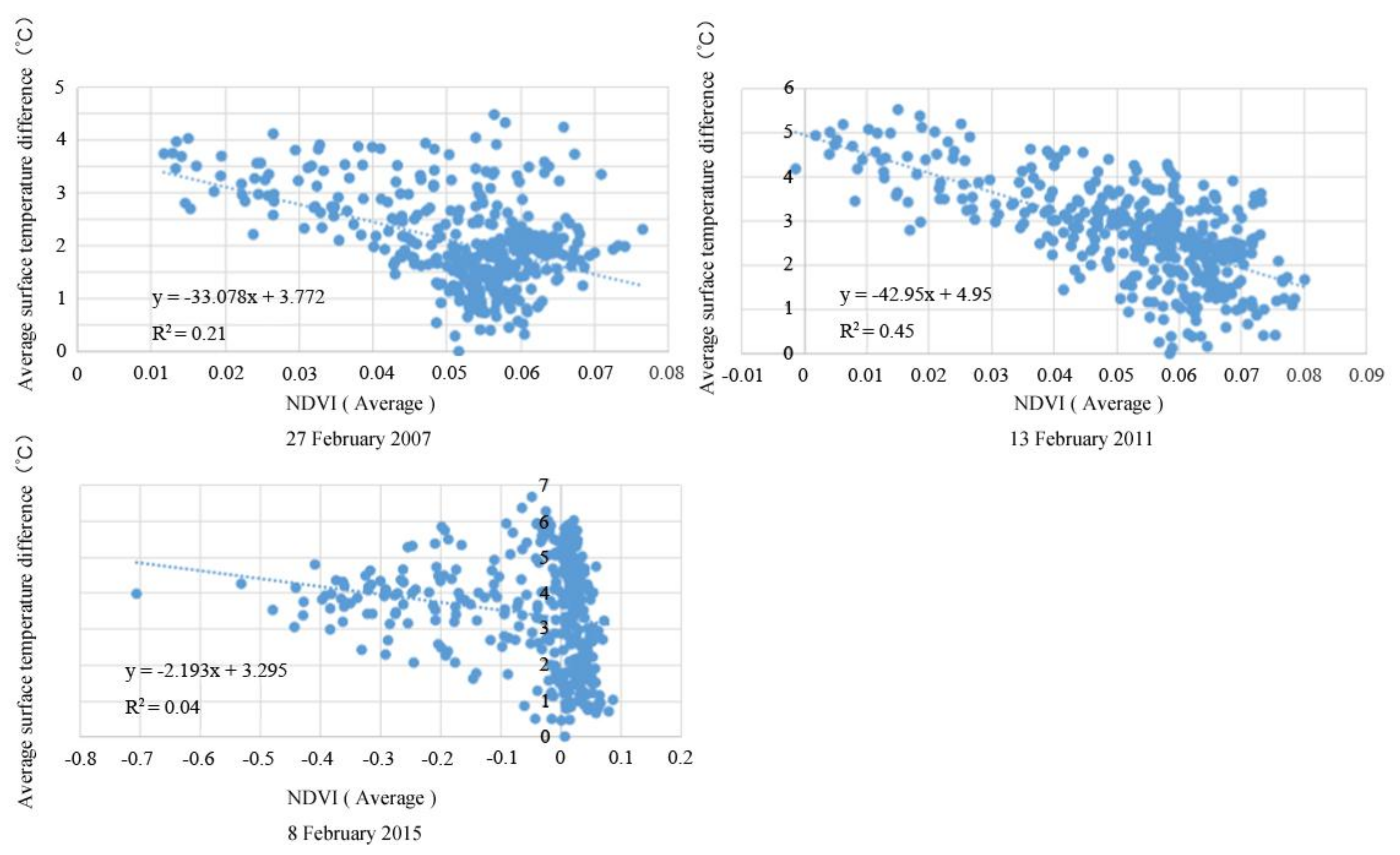
In winter, without snow cover, the urban green spaces have a certain mitigation effect on the UHI effects, which is far less significant than that in summer. Snow in severely cold areas, changes of underlying surface and the heat supply all affect the surface temperature difference and the UHI effect. From Figure 13 we can see the regression equation between the average surface temperature differences and the NDVI values is linear and the slope is negative, indicating that the surface temperature difference would decrease as the NDVI values increase. Through the extraction of the data in the winter of 2015, when the surface was not covered with snow, it was found that the surface temperature difference took on a bulk distribution like the NDVI value when it is smaller than 0. When the NDVI is between 0 and 0.1, the regression coefficient R2 achieves 0.031, indicating that when the NDVI value is larger than 0, the surface temperature difference has certain relevancy with the urban green spaces. The slope for the regression equation in winter is far smaller than that in summer. However, the change of NDVI values in winter have not surpassed 10% of those in summer. Therefore, the mitigation extent of the green spaces in winter is far less than that in summer. When the surface was covered by snow, the regression equation between the surface temperatures and the 2015 winter NDVI values were fitted and the correlation coefficient R2 was only 0.04. When the average NDVI is smaller than zero, the surface temperature differences took on the bulk distribution. This result indicates that when the surface was covered by snow the surface temperature difference had no significant relevance with the NDVI values that might be tightly correlated with other factors.
4.2. Implications for Urban Planning
The effects of area, perimeter and shape factor of green space on the UHI effect can be summarized as below.
- (1)
- Area effect. In summer within the range of 37 ha, the cooling extent, cooling distance and MTD are in significant positive correlation with the area. Beyond the area of 37 ha, a cooling effect of area is not obvious. In contrast, in winter a change of area would not affect the cooling distance significantly.
- (2)
- Perimeter effect. In summer, the cooling extent, cooling distance and MTD are in positive correlation with the perimeter in the range of 5300 m, while in winter, the cooling distance is nearly irrelevant to the perimeter.
- (3)
- Shape factor effect. In summer, the cooling extent, cooling distance and MTD are in positive correlation with the shape factor in the range of 0.03.
Since previous studies have mainly focused on tropical and temperate zones, they have focused less on sub-frigid and frigid zones [34]. In summer it was found in this work that for cities like Harbin in the cold zone, the area, perimeter and shape factor have a strong correlation with MTD with R2 values of 0.67, 0.61, 0.54, respectively. This conclusion is consistent with previous studies; it is noteworthy that the MTD in the sub-frigid zone in summer is higher than that in other zones. Moreover, the area, perimeter and shape factor have a certain correlation with the cooling distance with relatively lower R2 values of 0.45, 0.41 and 0.40, respectively. Noticeably, for the cooling extent, compared with the perimeter and shape factor, area has more effect with an R2 value of 0.63. The R2 values for the perimeter and shape factor are 0.53 and 0.48, respectively.
Few studies have referred to the cooling effect of green spaces in winter with temperatures lower than zero degrees. It is comprehensively accepted that the relevant study is meaningless. While in this work, it was found that in winter the UHI effect becomes stronger and the green spaces also possess a cooling effect. This is attributed to the large areas of snowfall in winter reflecting the radiation of sunlight, leading to a surface temperature that is lower than that of the underlying surface. The surrounding temperatures of green spaces would be therefore be lower than those in the areas with high-density buildings. The comfort of green spaces is unfavorable and the regional wind speeds are high. Therefore, it is meaningful to consider the effect of green spaces on temperature for urban design.
Considering the cooling effect of green spaces in summer and winter, increasing the area, perimeter and choosing a regular shape would improve the cooling effect. It is noteworthy that green spaces would not directly affect the cooling distance but would decrease the temperature. Therefore, to improve comfort, large-area green spaces are not recommended. Comprehensively, the scattering of green spaces should be uniform with a total area of 37 ha and perimeter of 5300 m, to obtain the optimum cooling effect. Besides, the shape of green spaces should be as neat as possible.
5. Conclusions
The cooling effect of urban green space in Harbin to reduce the UHI effect was carefully studied in this work. Three main factors, green space area, perimeter and shape factor, were found to predominantly affect the cooling effect of the green spaces, which were examined in summer and winter. In summer, the cooling effect is more significant. The average cooling extent reached 1.65 °C, the average maximum temperature change was 7.5 °C, and the cooling range was mainly 120 m. The cooling effect can be improved by increasing the green space area and perimeter. Increasing the green area (within 37 ha) or the green circumference (within 5300 m) can improve its cooling effect with minimum economic cost. Moreover, the cooling effect could be increased by reducing the shape factor (within 0.03). The simpler the green space shape, the more obvious the cooling effect. In contrast, in winter green spaces have a certain extent of cooling effect when there is little or no snow cover, although it is still less significant compared to the situation in summer. The average cooling extent reaches 0.48 °C, the average maximum temperature change is 4.25 °C, and the cooling range is mainly 90 m. There is no correlation between urban green space and the UHI effect in areas mainly covered by ice and snow. No matter whether in summer or winter, NDVI basically has a negative relationship with the UHI effect. This work could provide feasible protocols for urban green space design to effectively control the UHI effect of sub-frigid cities like Harbin.
Acknowledgments
This work is supported by the Project of Chinese National Natural Science Foundation—Study on the principle and design method of urban microclimate regulation in severe cold region. (Grant No. 51438005).
Author Contributions
P.C. and X.H. conceived and designed the experiments; P.C. performed the experiments; X.H. analyzed the data; M.H. contributed reagents/materials/analysis tools; P.C. wrote the paper.
Conflicts of Interest
The authors declare no conflict of interest.
References
- Oke, T.R. The energetic basis of the urban heat island. Q. J. R. Meteorol. Soc. 1982, 108, 1–24. [Google Scholar] [CrossRef]
- Jin, H.; Cui, P.; Wong, N.H.; Ignatius, M. Assessing the Effects of Urban Morphology Parameters on Microclimate in Singapore to Control the Urban Heat Island Effect. Sustainability 2018, 10, 206. [Google Scholar] [CrossRef]
- Santamouris, M. Heat island research in Europe: The state of the art. Adv. Build. Energy Res. 2007, 1, 123–150. [Google Scholar] [CrossRef]
- Zaksek, K.; Bechtel, B. Source area estimation of urban air temperatures. Urban Remote Sensing Event IEEE 2015, 1–4. [Google Scholar] [CrossRef]
- Oliveira, S.; Andrade, H.; Vaz, T. The cooling effect of green spaces as a contribution to the mitigation of urban heat: A case study in Lisbon. Build. Environ. 2011, 46, 2186–2194. [Google Scholar] [CrossRef]
- Bowler, D.E.; Buyung-Ali, L.; Knight, T.M.; Pullin, A.S. Urban greening to cool towns and cities: A systematic review of the empirical evidence. Landsc. Urban Plan. 2010, 97, 147–155. [Google Scholar] [CrossRef]
- Alavipanah, S.; Wegmann, M.; Qureshi, S.; Weng, Q.; Koellner, T. The role of vegetation in mitigating urban land surface temperatures: A case study of Munich, Germany during the warm season. Sustainability 2015, 7, 4689–4706. [Google Scholar] [CrossRef]
- Connors, J.P.; Galletti, C.S.; Chow, W.T.L. Landscape configuration and urban heat island effects: Assessing the relationship between landscape characteristics and land surface temperature in Phoenix, Arizona. Landsc. Ecol. 2013, 28, 271–283. [Google Scholar] [CrossRef]
- Zhou, W.; Huang, G.; Cadenasso, M.L. Does spatial configuration matter? Understanding the effects of land cover pattern on land surface temperature in urban landscapes. Landsc. Urban Plan. 2011, 102, 54–63. [Google Scholar] [CrossRef]
- Feyisa, G.L.; Dons, K.; Meilby, H. Efficiency of parks in mitigating urban heat island effect: An example from Addis Ababa. Landsc. Urban Plan. 2014, 123, 87–95. [Google Scholar] [CrossRef]
- Hamada, S.; Tanaka, T.; Ohta, T. Impacts of land use and topography on the cooling effect of green areas on surrounding urban areas. Urban For. Urban Green. 2013, 12, 426–434. [Google Scholar] [CrossRef]
- Bao, T.; Li, X.; Zhang, J.; Zhang, Y.; Tian, S. Assessing the distribution of urban green spaces and its anisotropic cooling distance on urban heat island pattern in Baotou, China. ISPRS Int. J. Geo-Inf. 2016, 5, 12. [Google Scholar] [CrossRef]
- Doick, K.J.; Peace, A.; Hutchings, T.R. The role of one large green space in mitigating London’s nocturnal urban heat island. Sci. Total Environ. 2014, 493, 662–671. [Google Scholar] [CrossRef] [PubMed]
- Hamada, S.; Ohta, T. Seasonal variations in the cooling effect of urban green area on surrounding urban areas. Urban For. Urban Green. 2010, 9, 15–24. [Google Scholar] [CrossRef]
- Yan, H.; Fan, S.; Guo, C.; Wu, F.; Zhang, N.; Dong, L. Accessing the effects of landscape design parameters on intra-urban air temperature variability: The case of Beijing, China. Build. Environ. 2014, 76, 44–53. [Google Scholar] [CrossRef]
- Yokobori, T.; Ohta, S. Effect of land cover on air temperatures involved in the development of an intra-urban heat island. Clim. Res. 2009, 39, 61–73. [Google Scholar] [CrossRef]
- Wong, N.H.; Yu, C. Study of green areas and urban heat island in a tropical city. Habitat Int. 2005, 29, 547–558. [Google Scholar] [CrossRef]
- Yu, C.; Hien, W.N. Thermal benefits of city parks. Energy Build. 2006, 38, 105–120. [Google Scholar] [CrossRef]
- Li, X.; Zhou, W.; Ouyang, Z.; Xu, W.; Zheng, H. Spatial pattern of green space affects land surface temperature: Evidence from the heavily urbanized Beijing metropolitan area, China. Landsc. Ecol. 2012, 27, 887–898. [Google Scholar] [CrossRef]
- Grahn, P.; Stigsdotter, U.K. The relation between perceived sensory dimensions of urban green space and stress restoration. Landsc. Urban Plan. 2010, 94, 264–275. [Google Scholar] [CrossRef]
- Wang, Y.; Zhan, Q.; Ouyang, W. Impact of Urban Climate Landscape Patterns on Land Surface Temperature in Wuhan, China. Sustainability 2017, 9, 1700. [Google Scholar] [CrossRef]
- Maimaitiyiming, M.; Ghulam, A.; Tiyip, T.; Pla, F.; Latorre-Carmona, P.; Halik, Ü.; Sawut, M.; Caetano, M. Effects of green space spatial pattern on land surface temperature: Implications for sustainable urban planning and climate change adaptation. ISPRS J. Photogramm. Remote Sens. 2014, 89, 59–66. [Google Scholar] [CrossRef]
- Li, X.; Zhou, W.; Ouyang, Z. Relationship between land surface temperature and spatial pattern ofgreenspace: What are the effects of spatial resolution? Landsc. Urban Plan. 2013, 114, 1–8. [Google Scholar] [CrossRef]
- Kong, F.; Yin, H.; James, P.; Hutyra, L.R.; He, H.S. Effects of spatial pattern of green space on urban cooling in a large metropolitan area of eastern China. Landsc. Urban Plan. 2014, 128, 35–47. [Google Scholar] [CrossRef]
- Bahi, H.; Rhinane, H.; Bensalmia, A.; Fehrenbach, U.; Scherer, D. Effects of urbanization and seasonal cycle on the surface urban heat island patterns in the coastal growing cities: A case study of Casablanca, Morocco. Remote Sens. 2016, 8, 829. [Google Scholar] [CrossRef]
- Alcoforado, M.J.; Andrade, H.; Lopes, A.; Vasconcelos, J. Application of climatic guidelines to urban planning: The example of Lisbon (Portugal). Landsc. Urban Plan. 2009, 90, 56–65. [Google Scholar] [CrossRef]
- Geletič, J.; Lehnert, M.; Dobrovolný, P. Land Surface Temperature Differences within Local Climate Zones, Based on Two Central European Cities. Remote Sens. 2016, 8, 788. [Google Scholar] [CrossRef]
- Hoflfinann, P.; Krueger, O.; Schlunzen, K.H. A statistical model for the urban heat island and its application to a climate change scenario. Int. J. Climatol. 2012, 32, 1238–1248. [Google Scholar]
- Sobrino, J.A.; Oltra-Carrio, R.; Soria, G.; Bianchi, R.; Paganini, M. Impact of spatial resolution and satellite overpass time on evaluation of the surface urban heat island effects. Remote Sens. Environ. 2012, 117, 50–56. [Google Scholar] [CrossRef]
- Sismanidis, P.; Keramitsoglou, I.; Kiranoudis, C.T.; Bechtel, B. Assessing the capability of a downscaled urban land surface temperature time series to reproduce the spatiotemporal features of the original data. Remote Sens. 2016, 8, 274. [Google Scholar] [CrossRef]
- Wang, J.; Zhan, Q.; Guo, H. The Morphology, Dynamics and Potential Hotspots of Land Surface Temperature at a Local Scale in Urban Areas. Remote Sens. 2016, 8, 18. [Google Scholar] [CrossRef]
- Ren, Z.; He, X.; Zheng, H.; Zhang, D.; Yu, X.; Shen, G.; Guo, R. Estimation of the relationship between urban park characteristics and park cool island intensity by remote sensing data and field measurement. Forests 2013, 4, 868–886. [Google Scholar] [CrossRef]
- Li, J.; Song, C.; Cao, L.; Zhu, F.; Meng, X.; Wu, J. Impacts of landscape structure on surface urban heat islands: A case study of Shanghai, China. Remote Sens. Environ. 2011, 115, 3249–3263. [Google Scholar] [CrossRef]
- Rasul, A.; Balzter, H.; Smith, C.; Remedios, J.; Adamu, B.; Sobrino, J.A.; Srivanit, M.; Weng, Q. A Review on Remote Sensing of Urban Heat and Cool Islands. Land 2017, 6, 38. [Google Scholar] [CrossRef]
Figure 1.
Green space distribution.
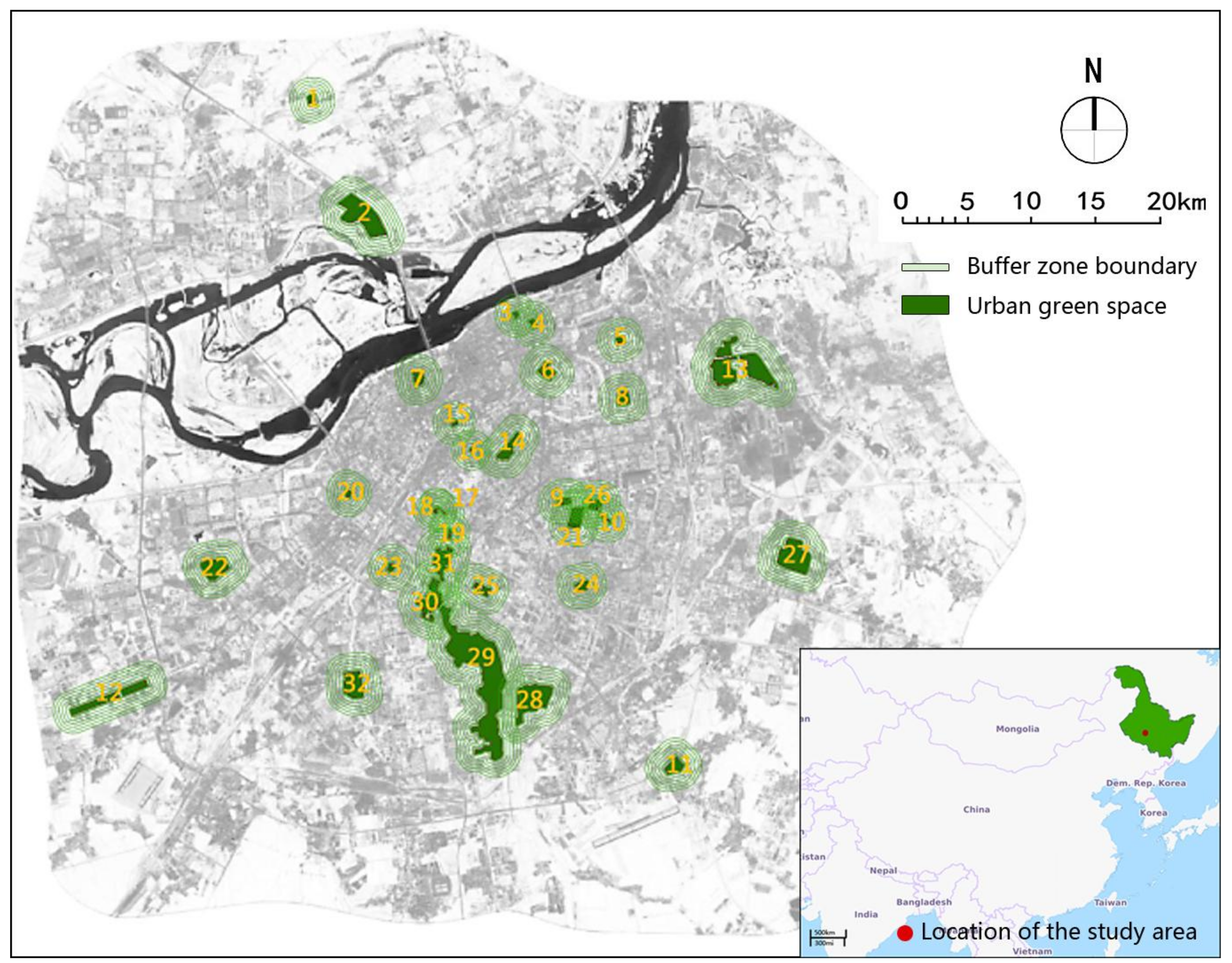
Figure 2.
Buffer zone settings.

Figure 3.
Intensity map of heat islands in Harbin. (a) 26 June2007; (b) 2 September 2011; (c) 18 July 2015; (d) 27 February 2007; (e) 13 February 2011; (f) 8 February 2015.
Figure 3.
Intensity map of heat islands in Harbin. (a) 26 June2007; (b) 2 September 2011; (c) 18 July 2015; (d) 27 February 2007; (e) 13 February 2011; (f) 8 February 2015.

Figure 4.
Intensity map of heat islands in Harbin in summer.

Figure 5.
Intensity map of heat islands in Harbin in winter.

Figure 6.
Correlation analysis between the cooling effect and the area of green space in summer.

Figure 7.
Correlation analysis between the cooling effect and the area of the green space in winter.
Figure 7.
Correlation analysis between the cooling effect and the area of the green space in winter.
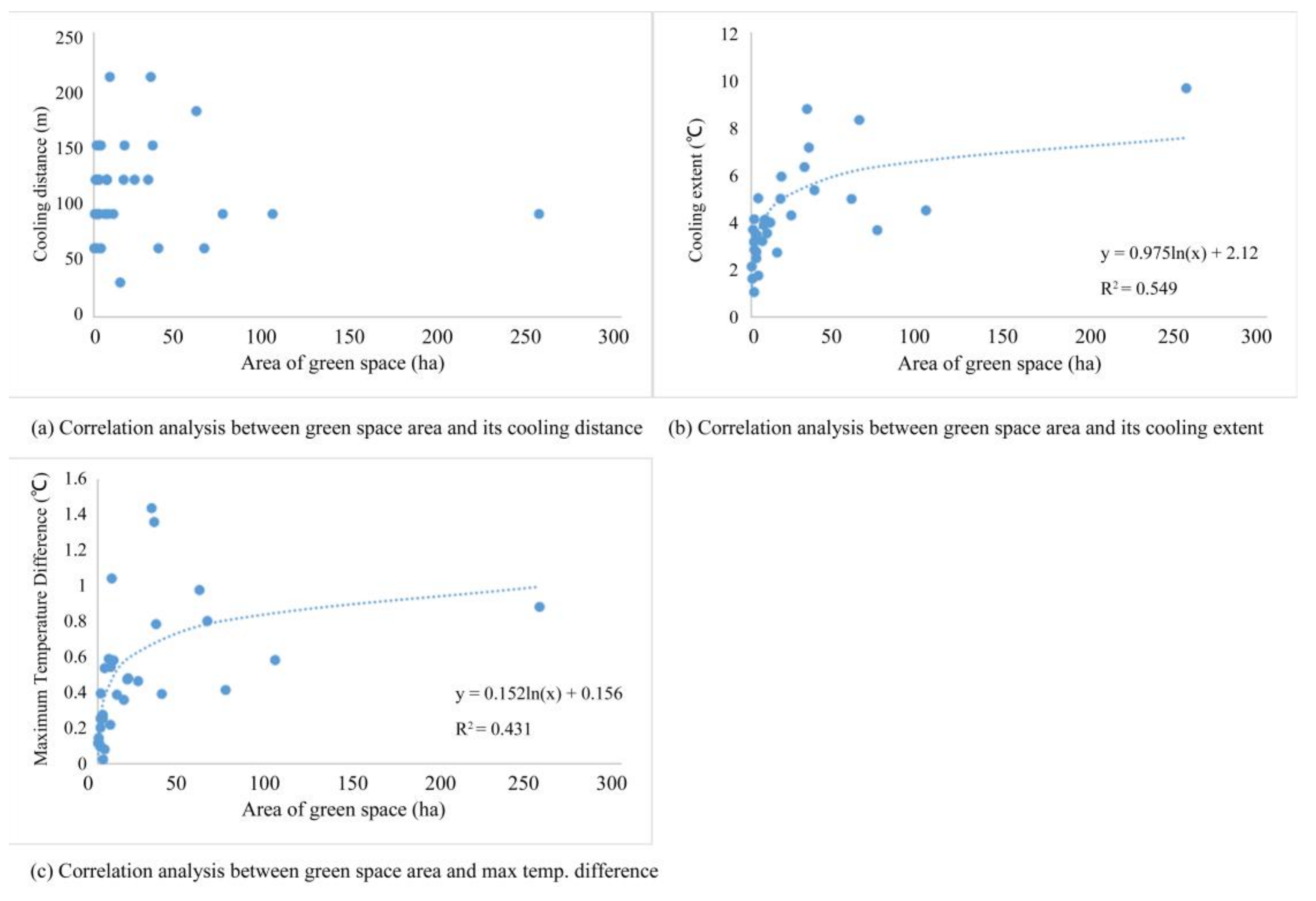
Figure 8.
Correlation analysis of the cooling effect and the perimeter of a green space in summer.
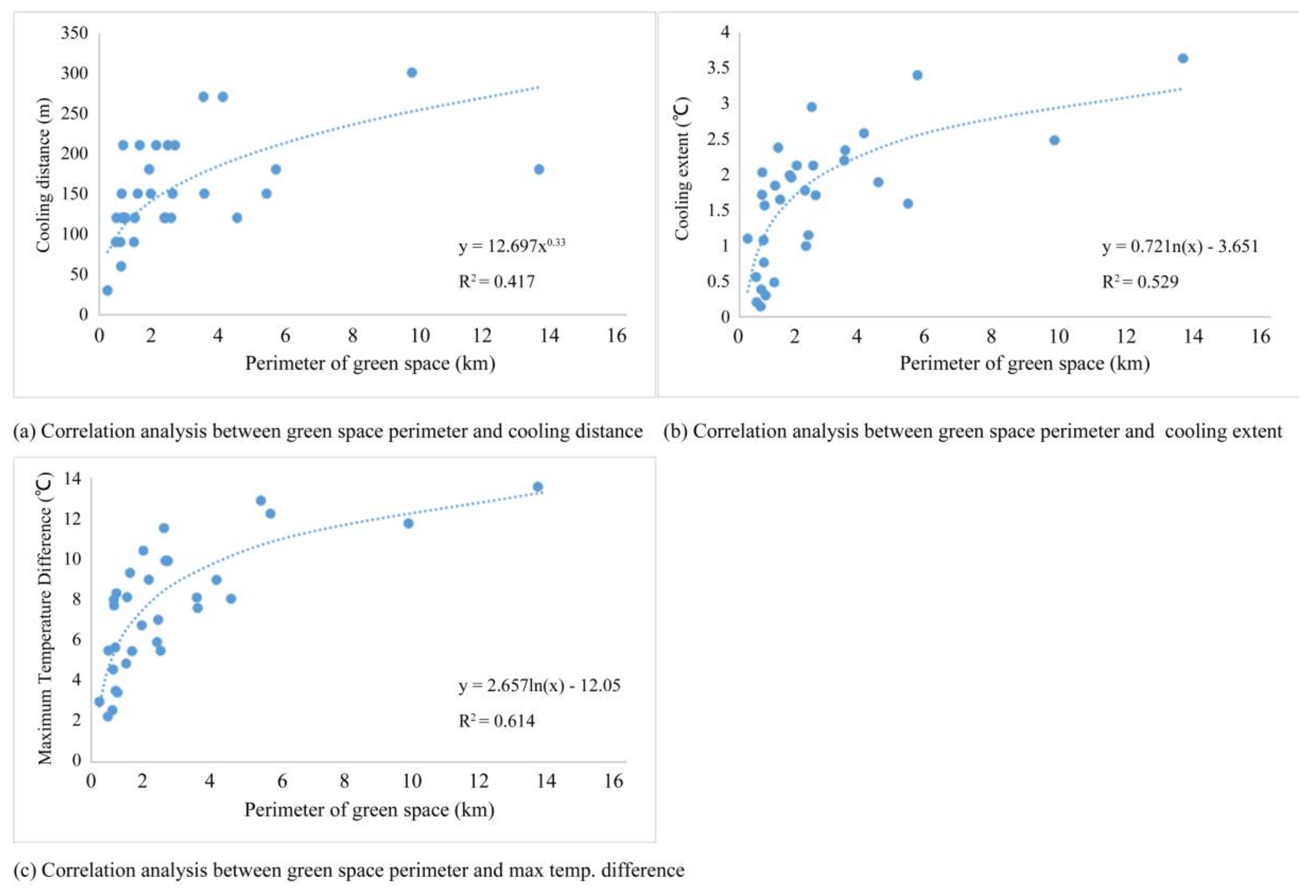
Figure 9.
Correlation analysis of the cooling effect and the perimeter of a green space in winter.
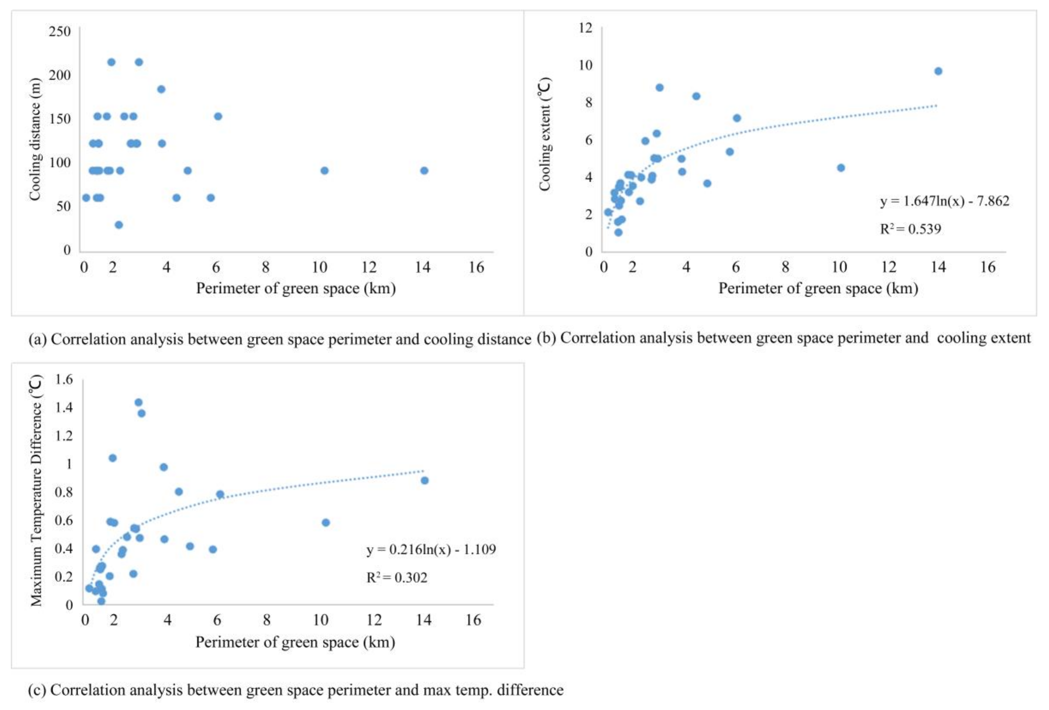
Figure 10.
Correlation analysis of the cooling effect and the shape factor of a green space in summer.
Figure 10.
Correlation analysis of the cooling effect and the shape factor of a green space in summer.
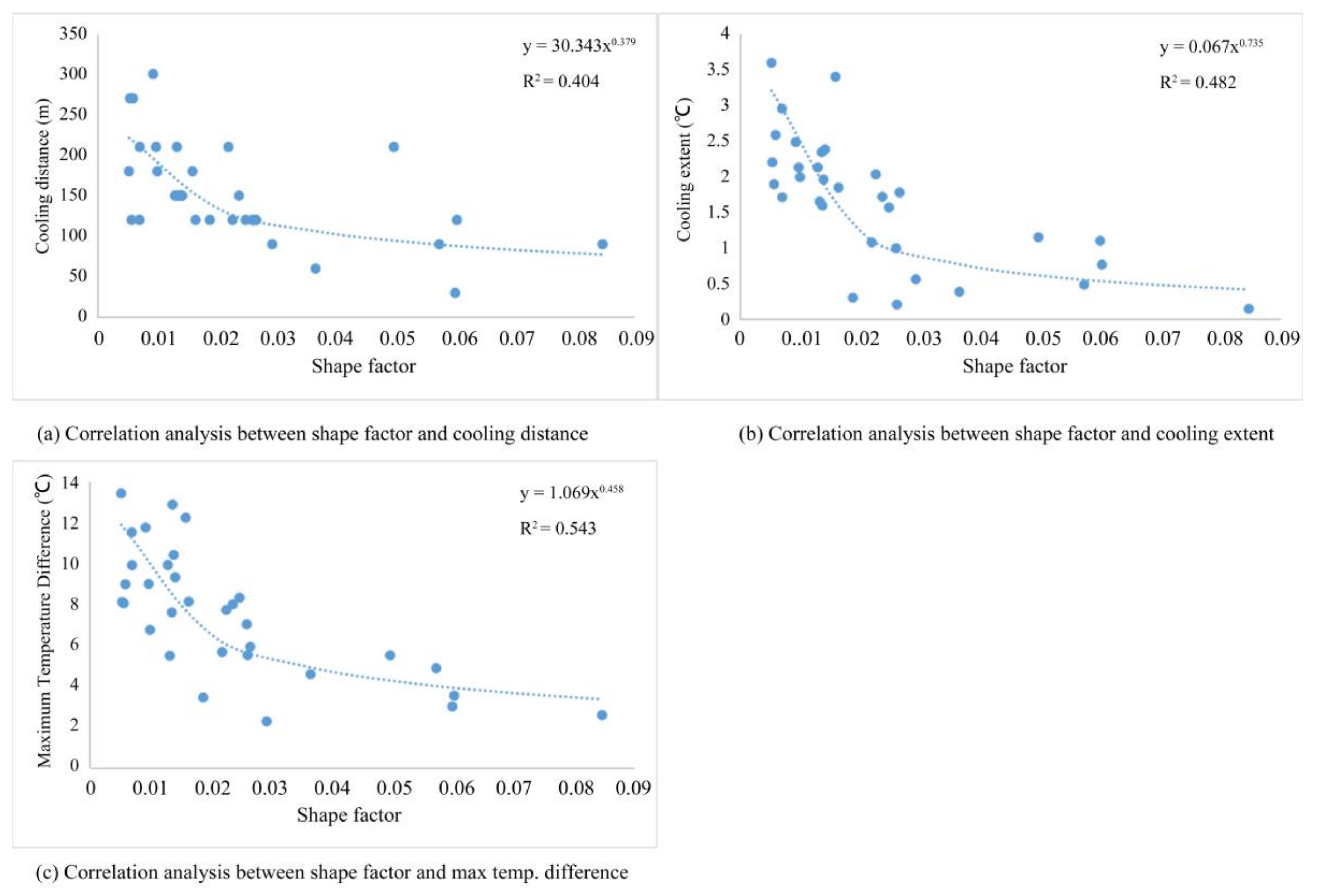
Figure 11.
Correlation analysis between cooling effect and the shape factor of green space in winter.
Figure 11.
Correlation analysis between cooling effect and the shape factor of green space in winter.
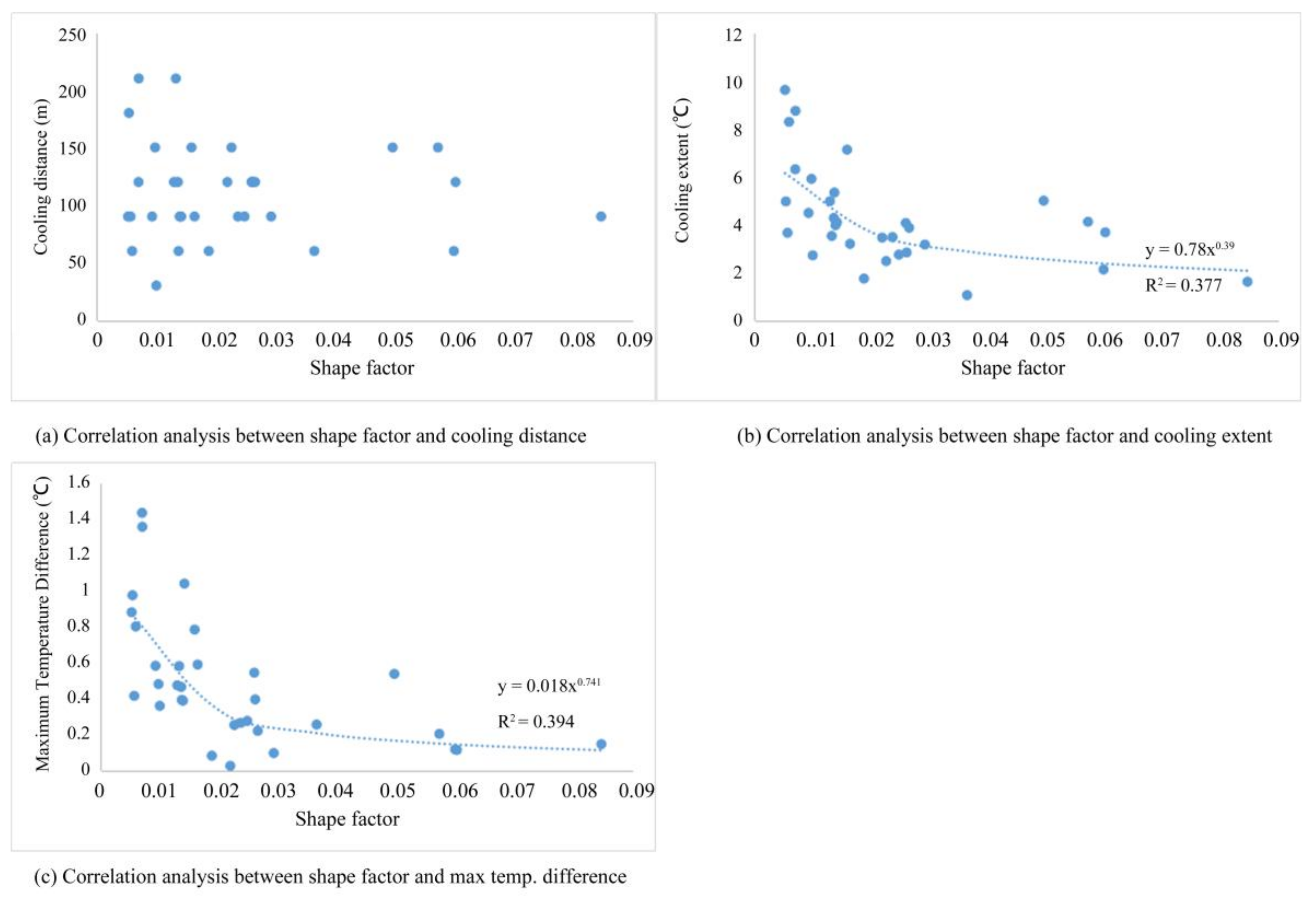
Figure 12.
Regression analysis of average surface temperature difference and NDVI in summer.
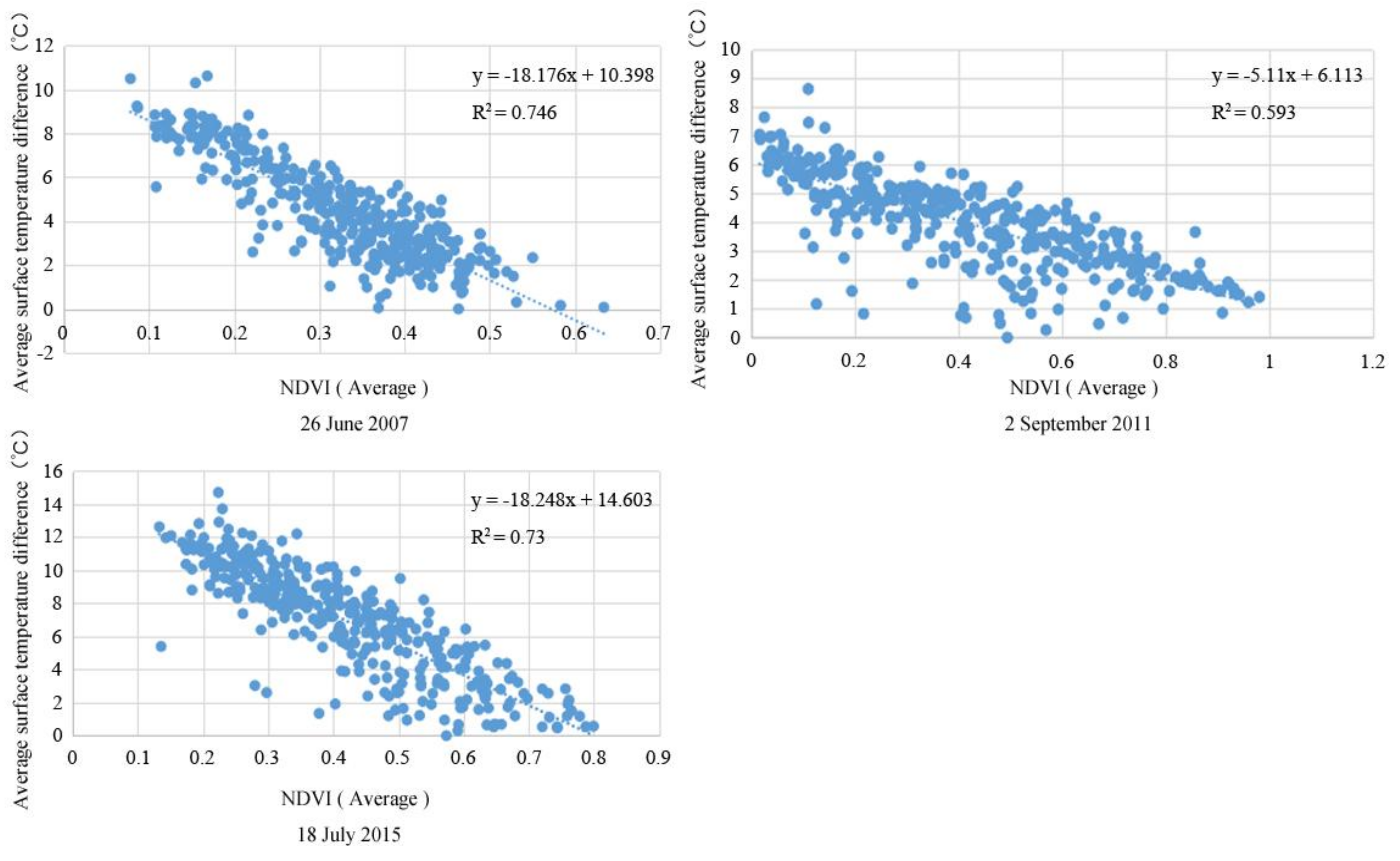
Figure 13.
Regression analysis of the average surface temperature difference and NDVI in winter.

Table 1.
Grading standard of UHIs.
| UHI Grade | Relative Temperature | Meaning |
|---|---|---|
| 1 | <−0.2 | Strong cold island (SCI) |
| 2 | −0.2–0 | Weak cold island (WCI) |
| 3 | 0–0.1 | Weak heat island (WHI) |
| 4 | 0.1–0.2 | Medium strong heat island (MSHI) |
| 5 | 0.2–0.4 | Strong heat island (SHI) |
| 6 | 0.4–0.6 | Extremely strong heat island (ESHI) |
Table 2.
The cooling effect of each selected green space cooling type.
| No | Urban Green Space | Area (ha) | Shape Factor | P (m) | Summer | Winter | ||||||
|---|---|---|---|---|---|---|---|---|---|---|---|---|
| CD (m) | CE (°C) | MTD (°C) | CT | CD (m) | CE (°C) | MTD (°C) | CT | |||||
| 16 | Memorial hall green space | 0.43 | 0.060 | 259 | 30 | 1.10 | 2.96 | PV | 60 | 2.11 | 0.12 | PV |
| 17 | Siling street green space | 0.77 | 0.085 | 648 | 90 | 0.14 | 2.54 | PV | 90 | 1.60 | 0.14 | PV |
| 18 | HIT green space | 1.24 | 0.060 | 747 | 120 | 0.76 | 3.49 | PV | 120 | 3.66 | 0.11 | PV |
| 3 | Guandao Park | 1.75 | 0.029 | 511 | 90 | 0.56 | 2.23 | PV | 90 | 3.15 | 0.09 | PV |
| 19 | Majia river green space | 1.83 | 0.037 | 670 | 60 | 0.38 | 4.54 | PV | 60 | 1.04 | 0.25 | PV |
| 11 | Heilongjiang law school Landscape | 1.85 | 0.057 | 1059 | 90 | 0.48 | 4.83 | PV | 150 | 4.10 | 0.20 | PV |
| 15 | Jihong bridge green space | 2.02 | 0.026 | 527 | 120 | 0.20 | 5.47 | PV | 120 | 2.82 | 0.39 | PV |
| 4 | Jingyu Park | 2.90 | 0.024 | 688 | 150 | 1.71 | 7.96 | LV | 90 | 3.46 | 0.26 | PV |
| 20 | Jianguo Park | 3.09 | 0.023 | 699 | 120 | 2.02 | 7.68 | PV | 150 | 2.46 | 0.25 | PV |
| 23 | Qinbin Park | 3.09 | 0.025 | 767 | 120 | 1.56 | 8.28 | PV | 90 | 2.73 | 0.27 | PV |
| 5 | Taiping Park | 3.34 | 0.022 | 733 | 210 | 1.07 | 5.62 | UV | 120 | 3.44 | 0.02 | PV |
| 9 | Development area Park | 4.20 | 0.050 | 2087 | 210 | 1.14 | 5.46 | UV | 150 | 4.98 | 0.53 | LV |
| 1 | Lvshanchuan Park | 4.25 | 0.019 | 800 | 120 | 0.30 | 3.40 | UV | 60 | 1.73 | 0.08 | UV |
| 24 | Shangzhi Park | 6.61 | 0.016 | 1085 | 120 | 1.84 | 8.09 | LV | 90 | 3.18 | 0.59 | LV |
| 25 | Heilongjiang medicine university | 7.45 | 0.027 | 1983 | 120 | 1.77 | 5.88 | PV | 120 | 3.85 | 0.22 | LV |
| 26 | Water supply company green space | 7.74 | 0.026 | 2014 | 120 | 0.99 | 6.98 | PV | 120 | 4.05 | 0.54 | PV |
| 7 | Zhaolin Park | 8.28 | 0.014 | 1175 | 150 | 2.37 | 9.28 | LV | 90 | 4.08 | 1.04 | LV |
| 8 | Old Pear Garden | 9.29 | 0.013 | 1236 | 210 | 1.64 | 5.44 | LV | 210 | 3.51 | 0.58 | UV |
| 6 | Culture Park | 11.27 | 0.014 | 1572 | 150 | 1.95 | 10.37 | LV | 90 | 3.96 | 0.39 | PV |
| 10 | Dingxiang Park | 15.21 | 0.010 | 1524 | 180 | 1.98 | 6.71 | PV | 30 | 2.70 | 0.36 | PV |
| 14 | Children’s park green space | 17.19 | 0.013 | 2232 | 150 | 2.12 | 9.88 | LV | 120 | 4.96 | 0.47 | LV |
| 21 | Golf Course | 17.70 | 0.010 | 1736 | 210 | 2.12 | 8.95 | UV | 150 | 5.89 | 0.48 | PV |
| 32 | Eurasian Park | 32.62 | 0.007 | 2304 | 210 | 1.70 | 9.87 | PV | 210 | 8.73 | 1.35 | UV |
| 31 | Science Park | 23.42 | 0.014 | 3195 | 150 | 2.33 | 7.56 | LV | 120 | 4.26 | 0.46 | PV |
| 22 | Qunli Park | 31.14 | 0.007 | 2187 | 120 | 2.94 | 11.48 | LV | 120 | 6.29 | 1.43 | PV |
| 30 | NEFU green space | 33.70 | 0.016 | 5368 | 180 | 3.39 | 12.19 | LV | 150 | 7.11 | 0.78 | PV |
| 12 | Airport Expressway Landscape | 36.96 | 0.014 | 5084 | 150 | 1.59 | 12.83 | PV | 60 | 5.32 | 0.39 | UV |
| 27 | Tangdu Garden | 58.57 | 0.005 | 3168 | 270 | 2.19 | 8.07 | PV | 180 | 4.95 | 0.97 | PV |
| 28 | Songle Park | 63.08 | 0.006 | 3758 | 270 | 2.57 | 8.94 | PV | 60 | 8.27 | 0.80 | PV |
| 2 | Tiger Garden | 73.58 | 0.006 | 4192 | 120 | 1.89 | 8.01 | PV | 90 | 3.64 | 0.41 | PV |
| 13 | Fengjiawazi Garden | 101.97 | 0.009 | 9492 | 300 | 2.48 | 11.71 | LV | 90 | 4.47 | 0.58 | PV |
| 29 | Forest botanical Garden | 253.60 | 0.005 | 13,351 | 180 | 3.58 | 13.38 | LV | 90 | 9.60 | 0.88 | PV |
Notes: The No. in the table is correspondence with the location in Figure 1 and the data is in ascending order by area index. Abbreviations: P = Perimeter; CD = Cooling Distance; CE = Cooling Extent; MTD = Maximum Temperature Difference; CT = Cooling Curve Type; UV = Uniform Variant; LV = Logarithmic Variant; PV = Parabola Variant.
Table 3.
The cooling effect of each selected green space cooling type.
| Cooling Curve Type | CE (°C) | Standard Deviation | MTD (°C) | Standard Deviation | ||||
|---|---|---|---|---|---|---|---|---|
| Summer | Winter | Summer | Winter | Summer | Winter | Summer | Winter | |
| UV | 1.16 | 0.60 | 0.75 | 0.54 | 5.86 | 4.82 | 2.30 | 2.99 |
| LV | 2.40 | 0.57 | 0.66 | 0.30 | 9.76 | 4.21 | 2.36 | 0.77 |
| PV | 1.29 | 0.44 | 0.76 | 0.34 | 6.43 | 4.16 | 2.86 | 2.08 |
Table 4.
The statistical frequency of different cooling distant and cooling curve type.
| CD (m) | 30 | 60 | 90 | 120 | 150 | 180 | 210 | 240 | 270 | 300 | |
|---|---|---|---|---|---|---|---|---|---|---|---|
| Summer | UV | 1 | 3 | ||||||||
| LV | 2 | 5 | 2 | 1 | 1 | ||||||
| PV | 1 | 1 | 3 | 7 | 1 | 1 | 3 | ||||
| Winter | UV | 1 | 1 | 1 | 1 | ||||||
| LV | 1 | 1 | 2 | 1 | |||||||
| PV | 1 | 3 | 8 | 5 | 4 | 1 | 1 |
Table 5.
The correlation coefficients between ΔLST and NDVI.
| Correlation | Pearson | Kendall | Spearman | |||
|---|---|---|---|---|---|---|
| Summer | Winter | Summer | Winter | Summer | Winter | |
| 2007 | −0.864 | −0.458 | −0.643 | −0.206 | −0.830 | −0.309 |
| 2011 | −0.770 | −0.668 | −0.611 | −0.446 | −0.797 | −0.623 |
| 2015 | −0.855 | −0.200 | −0.685 | −0.185 | −0.869 | −0.281 |
© 2018 by the authors. Licensee MDPI, Basel, Switzerland. This article is an open access article distributed under the terms and conditions of the Creative Commons Attribution (CC BY) license (http://creativecommons.org/licenses/by/4.0/).
Share and Cite
MDPI and ACS Style
Huang, M.; Cui, P.; He, X. Study of the Cooling Effects of Urban Green Space in Harbin in Terms of Reducing the Heat Island Effect. Sustainability 2018, 10, 1101. https://doi.org/10.3390/su10041101
AMA Style
Huang M, Cui P, He X. Study of the Cooling Effects of Urban Green Space in Harbin in Terms of Reducing the Heat Island Effect. Sustainability. 2018; 10(4):1101. https://doi.org/10.3390/su10041101
Chicago/Turabian StyleHuang, Meng, Peng Cui, and Xin He. 2018. "Study of the Cooling Effects of Urban Green Space in Harbin in Terms of Reducing the Heat Island Effect" Sustainability 10, no. 4: 1101. https://doi.org/10.3390/su10041101
Note that from the first issue of 2016, this journal uses article numbers instead of page numbers. See further details here.