Relationship between Spatio-Temporal Travel Patterns Derived from Smart-Card Data and Local Environmental Characteristics of Seoul, Korea

Department of Civil and Environmental Engineering, Yonsei University, Seoul 03722, Korea
*
Author to whom correspondence should be addressed.
Sustainability 2018, 10(3), 787; https://doi.org/10.3390/su10030787
Submission received: 29 January 2018
/
Revised: 9 March 2018
/
Accepted: 11 March 2018
/
Published: 13 March 2018
Abstract
:With the incorporation of an automated fare-collection system into the management of public transportation, not only can the quality of transportation services be improved but also that of the data collected from users when coupled with smart-card technology. The data collected from smart cards provide opportunities for researchers to analyze big data sets and draw meaningful information out of them. This study aims to identify the relationship between travel patterns derived from smart-card data and urban characteristics. Using seven-day transit smart-card data from the public-transportation system in Seoul, the capital city of the Republic of Korea, we investigated the temporal and spatial boarding and alighting patterns of the users. The major travel patterns, classified into five clusters, were identified by utilizing the K-Spectral Centroid clustering method. We found that the temporal pattern of urban mobility reflects daily activities in the urban area and that the spatial pattern of the five clusters classified by travel patterns was closely related to urban structure and urban function; that is, local environmental characteristics extracted from land-use and census data. This study confirmed that the travel patterns at the citywide level can be used to understand the dynamics of the urban population and the urban spatial structure. We believe that this study will provide valuable information about general patterns, which represent the possibility of finding travel patterns from individuals and urban spatial traits.
1. Introduction
The identification of urban structure is a topic that has long been studied by urban geographers and planners [1,2,3,4]. It is important to measure urban structures and identify the underlying activity pattern for the sake of supporting an evidence-based urban planning policy. Identifying activity centers, clusters and their characteristics not only gives urban planners a better understanding of the current structure of a city but also allows them to assess how their planning is being reflected [5].
In order to obtain a better understanding of the urban spatial structure, researchers have been increasingly scrutinizing urban mobility dynamics and their impact on urban environments, since the pattern of how people move about a city is closely related to urban spatial structures [6,7,8,9,10]. In the past, data was insufficient to analyze urban movement. However, in recent years, smart-card data from a public transportation system have opened a new opportunity to plot and understand urban dynamics. Consequently, as the data becomes more available, it has been facilitating spatial and temporal analysis of urban characteristics. Additionally, with the advances in technology, finer-resolution geospatial data have become available for modeling urban structures and dynamics [11,12].
Much literature has focused on the interrelationship between travel patterns and local environmental characteristics [13,14,15,16]. Much of the research on the link between the urban form and travel patterns belongs to the category of aggregate analysis [17,18]. Data aggregation could help screen idiosyncratic travel behaviors and identify the underlying fundamental aspects of human urban mobility [19]. Related studies have classified the travel patterns of public transportation passengers by using transit data. Ma et al. [20] defined five travel patterns extracted from the transit data of Beijing, China, through K-Means++ clustering. Goulet-Langlois et al. [21] classified 11 travel patterns from the users of London’s public-transportation network. Based on the travel pattern extracted from the transit data, several studies segmented urban areas to identify the underlying urban structure and regional functions. Yuan, Zheng, Xie, Wang, Zheng and Xiong [7] proposed a topic-modeling-based method to cluster the segmented regions into functional zones using taxi trajectories, public-transit data, points of interest (POIs), and road networks. Cats, Wang and Zhao [5] revealed urban structure dynamics using a spatial-temporal distribution of the public transportation passenger flow. Roth et al. [22] revealed the polycentric structure of London using smart-card data from the London Underground.
While previous studies highlighted the potential of smart-card data to classify travel patterns and urban forms, less is known about how point-based mobility data is distributed within urban areas. Generally, the data on the movement of people has been collected using point-based locations such as bus stops and subway stations. In most previous studies, the information of the point-based data (boarding and alighting counts) was simply summed over the unit area. However, problems can occur when the boarding and alighting point is not the final destination, which is the case for most passengers. Therefore, we developed the road-based mobility distribution model to distribute the point-based ridership within the unit area.
At the same time, it is important to examine whether mobility data are statistically meaningful to investigate the interrelation between human mobility and regional characteristics. In the case of Seoul, where using public transportation is more common than other equivalent cities, it is worthwhile analyzing public transportation data to identify the interrelation between urban mobility patterns and city characteristics. Additionally, due to the immense convenience of the public transportation system in Seoul, the usage of the transit smart card had increased to 98.9% by 2014 [23]. The transit smart card system generated about 20 million records daily; with stored passenger locations and time of ridership daily within the Seoul metropolitan area [24]. In this regard, we used smart-card data from the Korean automated fare collection (AFC) system to identify general travel patterns throughout the city, and investigated the interrelationship between travel patterns and urban spatial characteristics with land use and socio-demographic data. Our study will provide valuable information concerning the spatial and temporal characteristics of intra-urban mobility, the effect of built environments on travel patterns, and vice versa. We believe that this gives an insight into determining general patterns of geographical areas, as well as the traits of the areas.
The rest of the paper is organized as follows: Section 2 describes the study area and the datasets considered: smart-card data and local environmental data (land-use and socio-demographic data); Section 3 presents the methodology defined for the mobility-pattern analysis and its relationship to local environments; and the discussion and conclusion are given in Section 4 and Section 5, respectively.
2. Study Area and Data Preparation
2.1. Study Area
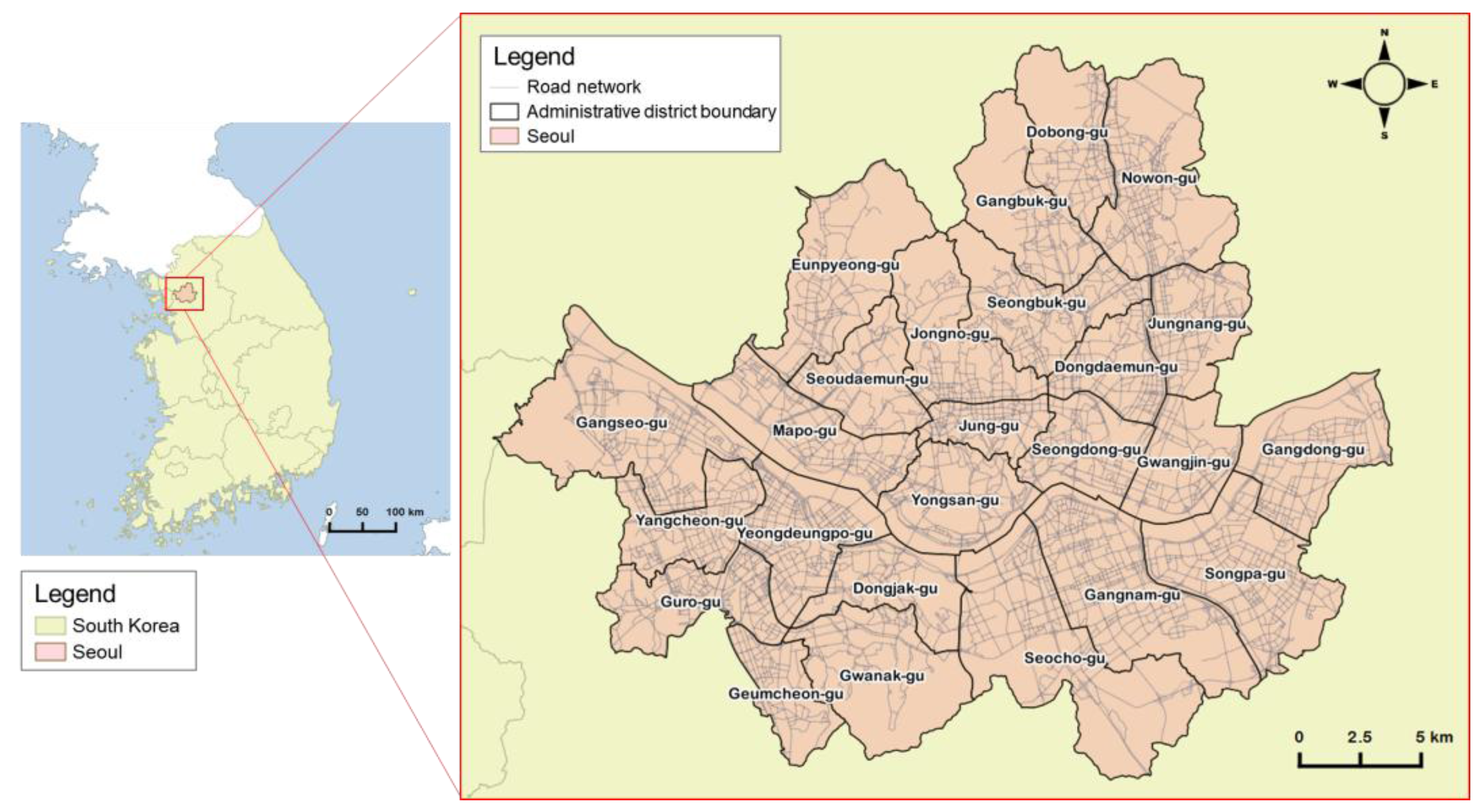
Seoul is a vibrant capital city that has historically attracted people and commerce. As a political and economic center, Seoul is the largest metropolis in and the capital of South Korea. The 2015 population of Seoul was 10.3 million and the metropolitan area had 25.5 million people, which is half the population of Korea [25]. At 605.2 km2, 0.6% the total area of Korea, and a population density of 17,014 persons per square kilometer, Seoul is one of the most densely populated cities in the world. It is comprised of 25 gu (local government districts) and the study area covers the entire city (Figure 1).
The Korean public transit system, including buses and subways, serves a large part of inter- and intra-city travel. Nine major subway lines and six different bus categories run throughout the city. In 2014, the public transportation system catered to about 55% of travel in Seoul (24.6% by bus, 10.5% by subway and train, and 19.4% by bus and subway) [26]. Accordingly, buses and metros play an essential part of urban trips in Seoul. Since transit smart-card usage of public transportation users in Seoul is close to 100%, as mentioned earlier, transit data produced from the study area is considered to be a reliable source of information for explaining the flows of urban passengers.
2.2. Smart-Card Data
The source data holds transit smart-card records from 18–24 March 2015, in Seoul. We used a data set that covers seven days consecutively from Monday to Sunday. The dataset used to describe urban mobility patterns covers the two major public transport modes, i.e., bus and subway. The smart-card data was gathered from 7 million smart cards of public transit users and contained about 20 million transport records daily. From the smart-card data, we could extract the time and the location of boarding and alighting without reference to the public transportation modes. Considering that we concentrated on the departure point and the destination point of a trip, we reorganized the smart-card records into a table form that contains initial boarding information and final alighting information. The arranged data consists of a transaction number, a boarding time, an ID of the boarding location, alighting time, an ID of the alighting location, and the number of passengers. The configuration of the arranged transit data is given in Table 1.
2.3. Local Environmental Data
The data sets used in this study also include socio-demographic statistics and a land-use land cover (LULC) map provided by Statistics Korea and the Korean Ministry of Environment (MOE). The socio-demographic statistics are provided on a census output area (OA) that is based on smaller blocks than administrative districts, and contain four main categories: population, household, housing, and business [27]. The socio-demographic data provided detailed information on the size, distribution and structure of population, housing, and businesses in Korea. LULC data contains detailed information on the urban area such as residential, industrial, commercial and recreational facilities areas. Table 2 shows the detailed information of the variables used.
2.4. Unit Area and Data Preparation
The socio-demographic data used in this study was provided on OA. OA in Korea is the smallest geographic unit for the publication of statistical data and is designed to contain approximately 500 residents [28]. Even though many studies use geographical areas as the unit of analysis, spatial units can greatly influence the result of a study, which is known as the modifiable areal unit problem (MAUP) [29].
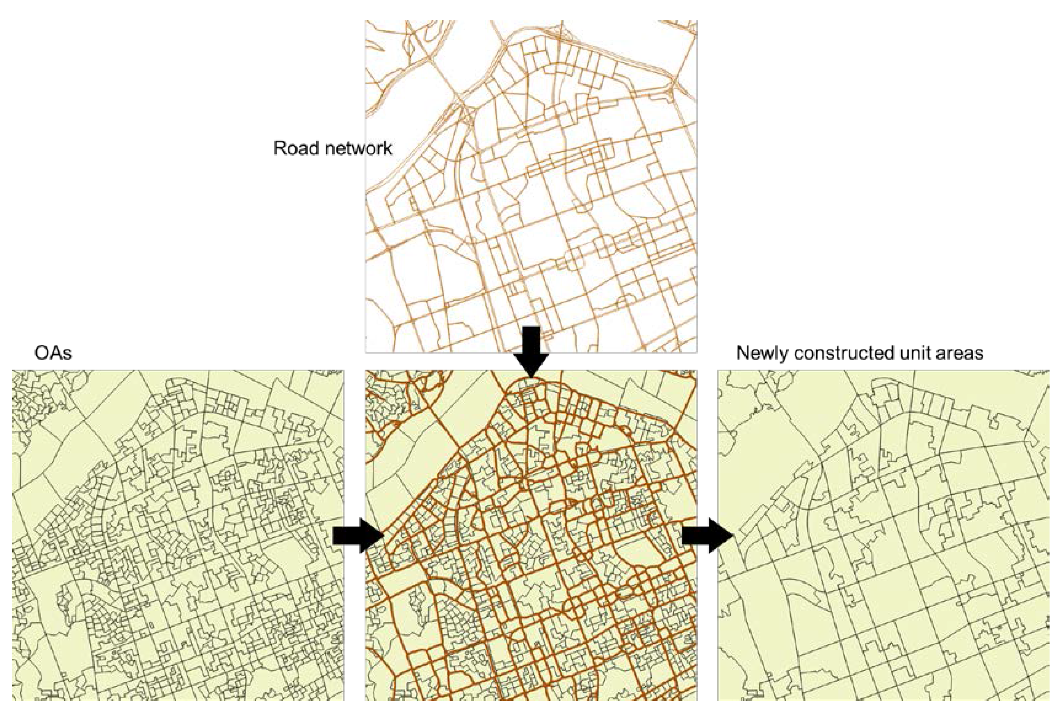
OAs and grids are widely used as the units of analysis. In urban environments, however, the segmentation of an urban area based on a road network is more natural than other criteria. Since people usually live in road-segmented regions and travel among road-segmented regions, we aggregated the OAs of the study area with the road network using the road-based segmentation method [30]. For this, we extracted the road-network data provided by the Korean Ministry of Land, Infrastructure and Transport (MOLIT). Aggregated OAs (AOAs) by the road network are considered as a basic unit of our study on the assumption that the road-segmented regions are the bases of daily activity and human mobility (Figure 2).
3. Methods
Methods include region clustering to identify the human-mobility patterns of Seoul and correspondence analysis (CA) to discover the relationships between human-mobility patterns and local environments. Figure 3 depicts the overall processing scheme of the study. Each step will be explained in detail in the following sections.
3.1. Aggregate Human-Mobility Patterns from Smart-Card Records
3.1.1. Road-Based Mobility Distribution
Boarding and alighting counts of transit records are represented as point-based, as listed in Table 1. For spatial clustering, counts of boarding and alighting in each unit area are needed for the calculation. For this, boarding and alighting counts inputted into unit areas (i.e., AOAs) are aggregated. In order to distribute the point-based ridership into each AOA, we used the street-weighting method that utilizes the vector street network [31,32]. The average walking distance of public transportation users, the distance from a station or a bus stop to users’ origin or destination, were 432 to 525 meters over the study area [33]. According to the Seoul Metropolitan City Planning Decree, the station influence area is defined as a 500-m radius from a station [34]. Accordingly, the point-based boarding and alighting data was redistributed into the street within a radius of 500 m, since we assumed that users of the public transportation travel on foot after getting on/off public transportation; the street network indicates the pedestrian level (Figure 4).
After distributing boarding and alighting of all stations/bus stops into the streets, boarding and alighting counts are recalculated within each AOA and accumulated at hourly intervals. Mathematically, we denote a transit data for each AOA , from time to , as given in Equation (1):
where and are sequences of boarding or alighting counts of time-stamped AOAs.
3.1.2. Clustering Analysis
Cluster analysis is a common approach for discovering the grouping of a set of patterns. Generally, clustering methods use distance measures, such as Euclidean distance or Manhattan distance, to define similarity among different objects. However, clustering in high-dimensional spaces is often problematic with those distance measures because distance functions are not always suitable for measuring correlation among the objects [35]. As the dimension of the data grow, the difference between close and distant objects becomes useless or some attribute values become insignificant in a given cluster [36].
Therefore, to derive a new distance-measurement scheme, we started with the notion that the arranged transit data consists of hourly boarding and alighting counts during seven days. Transit data arranged in Section 3.1.1 consists of hourly boarding and alighting counts during seven days. If we consider that the columns of the dataset are independent among others, 24 × 7 × 2 variables (24 h, 7 days, boarding and alighting) should be used for clustering. Since the pattern of human mobility behavior is very regular and diurnal, it is important to find distinct patterns by matching the similarity of data at the same time of day [37]. To do so, the distance measure as shown in Equation (2) was utilized. Based on one day (24 h), given two time series and , the distance between them is calculated:
where is the norm. The distance between a pair of time-series data can be regarded as an indicator to show the similarity between them. The smaller the distance, the higher the similarity becomes. Since the peak in the transit-data information at the given interval is also important, time series with for the same period were compared. As our data contains seven days and boarding/alighting components, the distance measure used can be represented as shown in Equation (3). In Equation (3), means the similarity measure of boarding/alighting data between th and th region during the given days:
Next, to find clusters of the time series that share a distinct temporal pattern, the K-SC clustering algorithm was chosen. K-SC, similar to K-means clustering, is an iterative algorithm that uses a time-series distance metric to calculate cluster centroids. K-SC computes more accurate and informative cluster centroids by matching the variation of time series data [38], which can be readily applied to identify common travel patterns from transit data.
3.1.3. Cluster Validity Measures
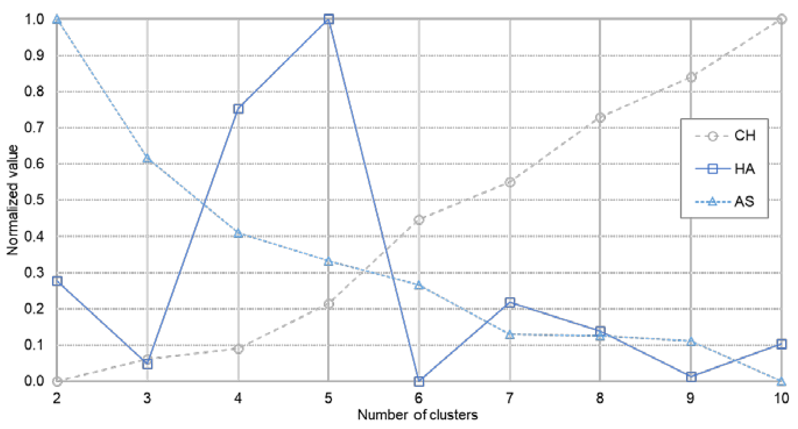
Determining the most appropriate number of clusters is one of the trying problems in cluster analysis. The K-SC algorithm, in common with other variants of K-means, needs the number of clusters (K) to be specified by users. To find the optimal number of clusters, numerous approaches have been suggested [39,40,41,42,43]. The common method for estimating the best number of clusters is to measure the quality of the clustering given a specific number of clusters with a criterion [44]. To measure the goodness of the clustering, various validation indices have been proposed. Since we could rely on the data itself for clustering, frequently-used internal clustering validation indices were used; the Calinski–Harabasz index [39], Hartigan’s Index [40], and the Average Silhouette [41], while implementing K-SC with a different number of clusters. Those clustering validation indices were compared to determine the optimal number of clusters for our study.
3.2. Relating Mobility Pattern and Local Environmental Characteristics
Principal component analysis (PCA) using the local environment data was utilized to analyze the socio-demographic data (population census, business, and land use). The reason for incorporating this procedure is that there are too many variables related to each other. By applying PCA, we were able to reduce the number of variables and reorganize the data sets. After reducing the variables, a multiple correspondence analysis (MCA) was implemented to find the relationship with mobility patterns.
3.2.1. Variable Reduction Using Principal Component Analysis (PCA)
PCA is a classical technique in statistical data analysis for data reduction. The purpose of PCA is for structuring many variables into a smaller number of components while retaining much of the information of the original data. Because variables from census data are often correlated with each other, PCA can be efficiently used for removing the collinearity of variables and uncovering latent variables [45]. There are a total of 142 local environmental variables including demographic, business and LULC characteristics, as summarized in Table 2. To simplify the structure of variables for further analysis, PCA was applied to extract fewer uncorrelated components. The resulting components are used as key variables in the next step.
3.2.2. Multiple Correspondence Analysis (MCA)
MCA is an extension of correspondence analysis, which is a statistical technique to analyze the interrelationships among several categorical dependent variables [46]. Correspondence analysis is suited for analyzing contingency tables, which examine the associations among variables. The distinct advantage of correspondence analysis is that it can be used to find the relationship within dependent variables or within independent variables, as well as the interrelationship between dependent variables and independent variables. It is useful to represent the interrelations among variables on a map [46,47]. The reason for applying MCA in our case is that it could reveal the relationship between mobility patterns and other variables without prior knowledge and provide insight into the relationships between them. Moreover, MCA could visualize the relationships between variables on the plane.
4. Results and Discussion
4.1. Clustering (Analysis of Human Activities from the Aggregated Perspective)
4.1.1. Clustering Validity
Figure 5 shows the values of the three measures, the Calinski–Harabasz index (CH), Hartigan’s Index (HA), and the Average Silhouette (AS), as a function of the number of clusters. We experimented with K = 2 to 10 and each measure was normalized from zero to one. The higher value indicates good clustering, but those measures do not always match each other. As shown in Figure 5, the tendency of CH and AS is the opposite but in case of HA, the value; when K = 5, is the highest. Since it implies that K = 5 gives the best clustering results, we chose K = 5 as the number of clusters for our data sets.
4.1.2. Temporal Pattern of Public-Transit Passengers
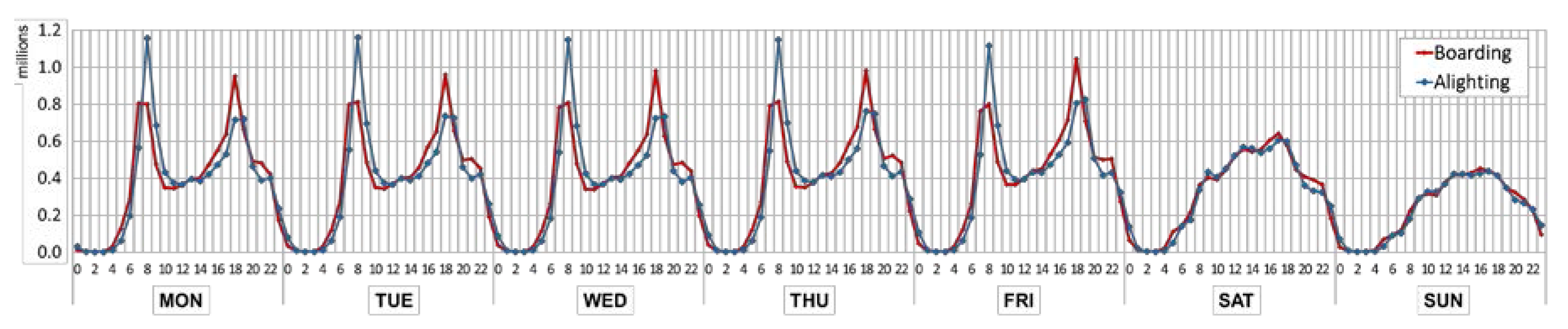
Figure 6 presents the total boarding and alighting counts of the study area: the temporal pattern for public transportation. The temporal pattern for public transportation refers to the boarding and alighting counts over time. The temporal pattern during weekdays exhibits a bimodal shape over a day. During the morning rush hour, the alighting pattern has the highest peak point between 08:00 and 09:00. In comparison, the boarding counts during 07:00–08:00 and 08:00–09:00 have similar values. During the evening rush hour, the boarding pattern has the highest peak point between 18:00 and 19:00 while the alighting counts during 18:00–19:00 and 19:00–18:00 are similar. This reflects commuting time from boarding to alighting, and clearly shows the use of public transportation for commuting during general working hours in Korea (09:00–18:00). Meanwhile, the temporal patterns during the weekend are much smoother than those of weekdays and similar for both boarding and alighting. The fact that the temporal patterns are grouped into two i.e., weekdays (Mon-Fri) and the weekend (Sat-Sun) can be visually identified.
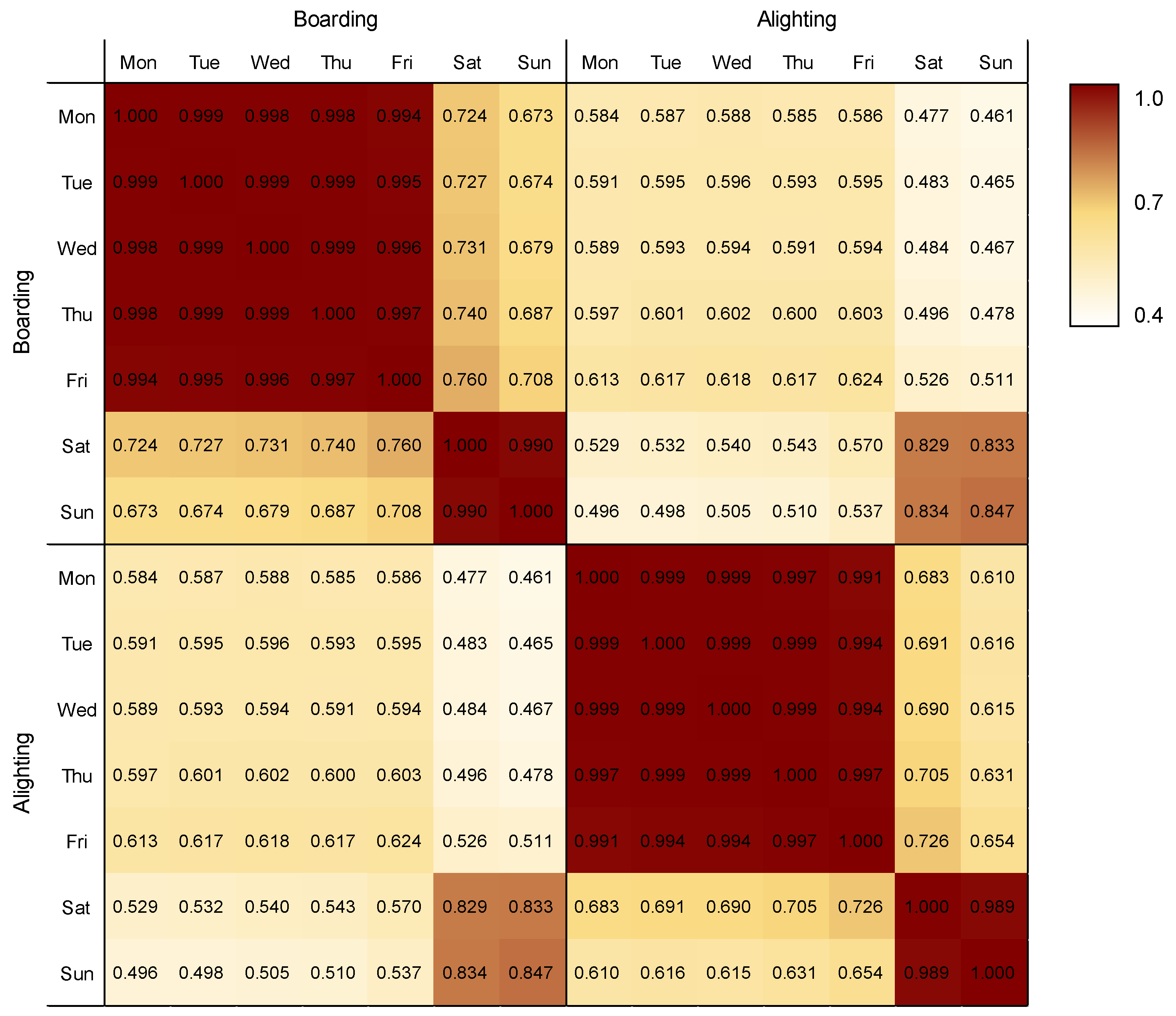
It can be numerically confirmed that the temporal patterns can be separated into two groups through Pearson’s correlation coefficients, as shown in Figure 7. In the case of weekdays, boarding or alighting patterns have strong correlations (0.991–0.999). For the weekend, temporal patterns are also highly correlated (0.989–0.990). Meanwhile, the correlation between boarding and alighting patterns of weekdays is relatively low (0.584–0.624); and the correlation between the boarding and alighting pattern of the weekend is higher than that of weekdays (0.829–0.847). Since the patterns between weekdays and the weekend are distinct, we further analyzed the commuting patterns using two categories (i.e., weekday and weekend).
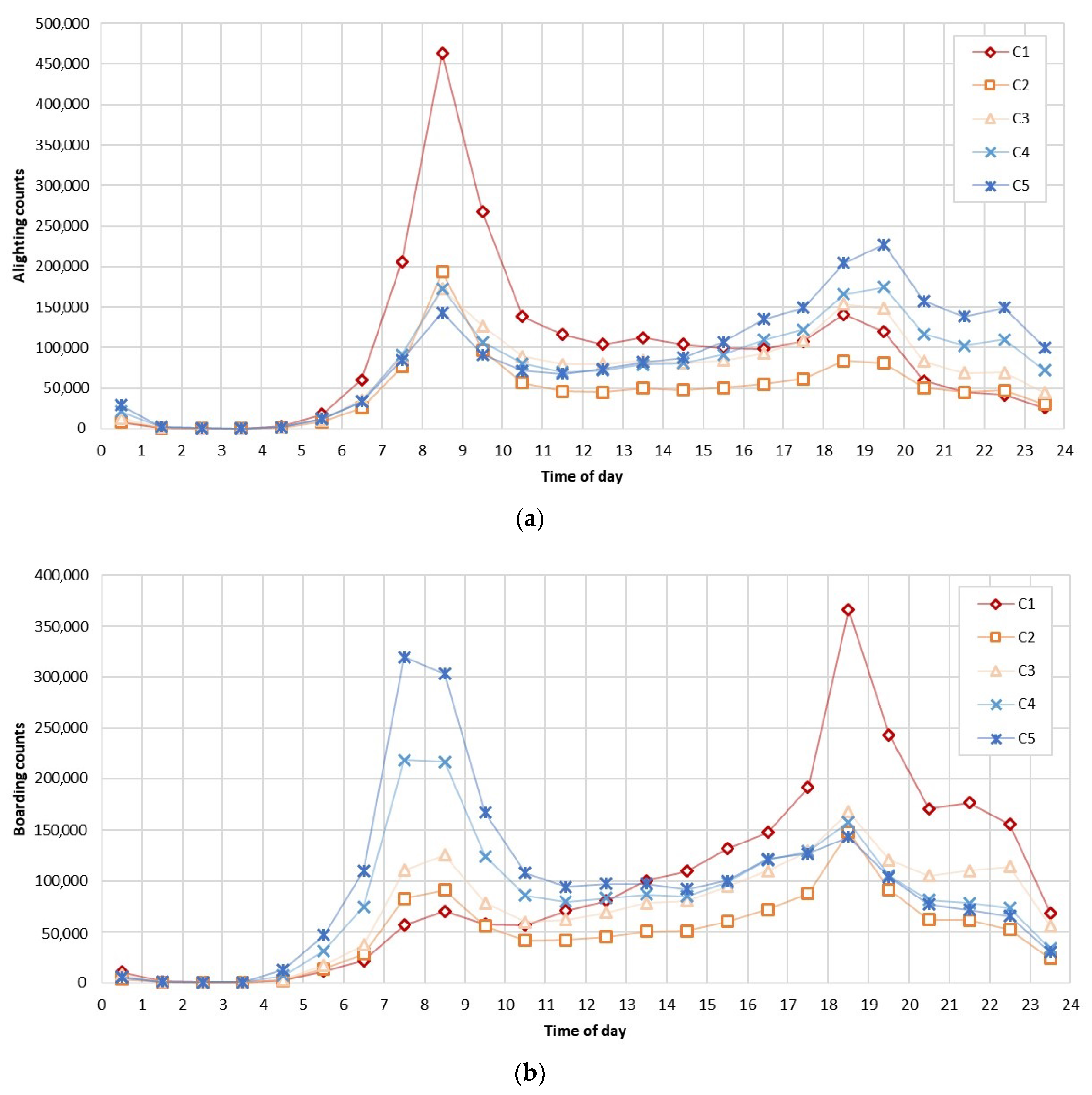
To investigate patterns of weekdays and the weekend, counts of five weekdays (Mon–Fri) and the weekend (Sat–Sun) were averaged and the results are shown in Figure 8 and Figure 9. Each cluster for K = 5 is labeled as C1, C2, C3, C4, and C5, respectively. The clusters were sorted out so that C1 is the largest and C5 is the smallest in the morning peak hour (the boarding peak volume is in an ascending order). In Figure 8, representing the temporal pattern of weekdays, the boarding of C1 begins to increase gradually in the morning and reaches its peak between 18:00–19:00. Meanwhile, the alighting of C1 soars rapidly in the morning and decreased after that time. Moreover, the peaks of C1 is the highest in both boarding and alighting. It means that C1 has many incoming passengers in the morning and many people outgoing in the evening. In the case of C2, the boarding in the morning is slightly high higher than C1 but the peak in the evening is less than half of that of C1. And C2 has the lowest public transport passengers in the middle of the day. The boarding and alighting patterns of C3 are similar to those of C1 and C2, but there is a difference in the boarding pattern of C3 at 22:00. C3 has a third peak point at night and it means more people stay in C3 than in C2 in the evening. In the case of C4, the boarding peak in the morning exceeds the peak in the evening. C5 shows a similar tendency, but its boarding in the morning and alighting in the evening are higher than those of C4. This signifies that many people leave C4 and C5 in the morning and arrive in the evening to night periods.
Figure 9 shows the temporal pattern of boarding and alighting during the weekend. Unlike the pattern of weekdays, the diurnal pattern of the weekend shows a unimodal shape. Compared to the patterns of weekdays with peak points in the morning or evening, the patterns of the weekend have peak points during the daytime. It can be inferred that the movement patterns of people during the weekend and weekdays are significantly different. In addition, the shapes of boarding and alighting during the weekend are relatively similar.
In C1, there was a great influx of people between 09:00 and 14:00 and many people moved out of C1 from late afternoon until night. Also, the highest peak points of boarding and alighting are in C1, which means many people visit C1 during the weekend as well as weekdays. C2 has the least percentage of people who utilize public transport, exhibiting no discernible peaks. C3 showed a similar pattern with C1, having higher alighting counts than C1 in the evening to night. C2 is the region that attracts a substantial number of people even later in the evening. C4 and C5 have opposite trends of C1 and C2. Although the boarding and alighting of C5 is higher than those of C4, their patterns are similar to each other. Lots of people ride public transportation in the morning and alight in the evening; many people in C4 and C5 leave these areas in the morning and return in the evening to night.
4.1.3. Temporal Pattern of Public-Transit Passengers
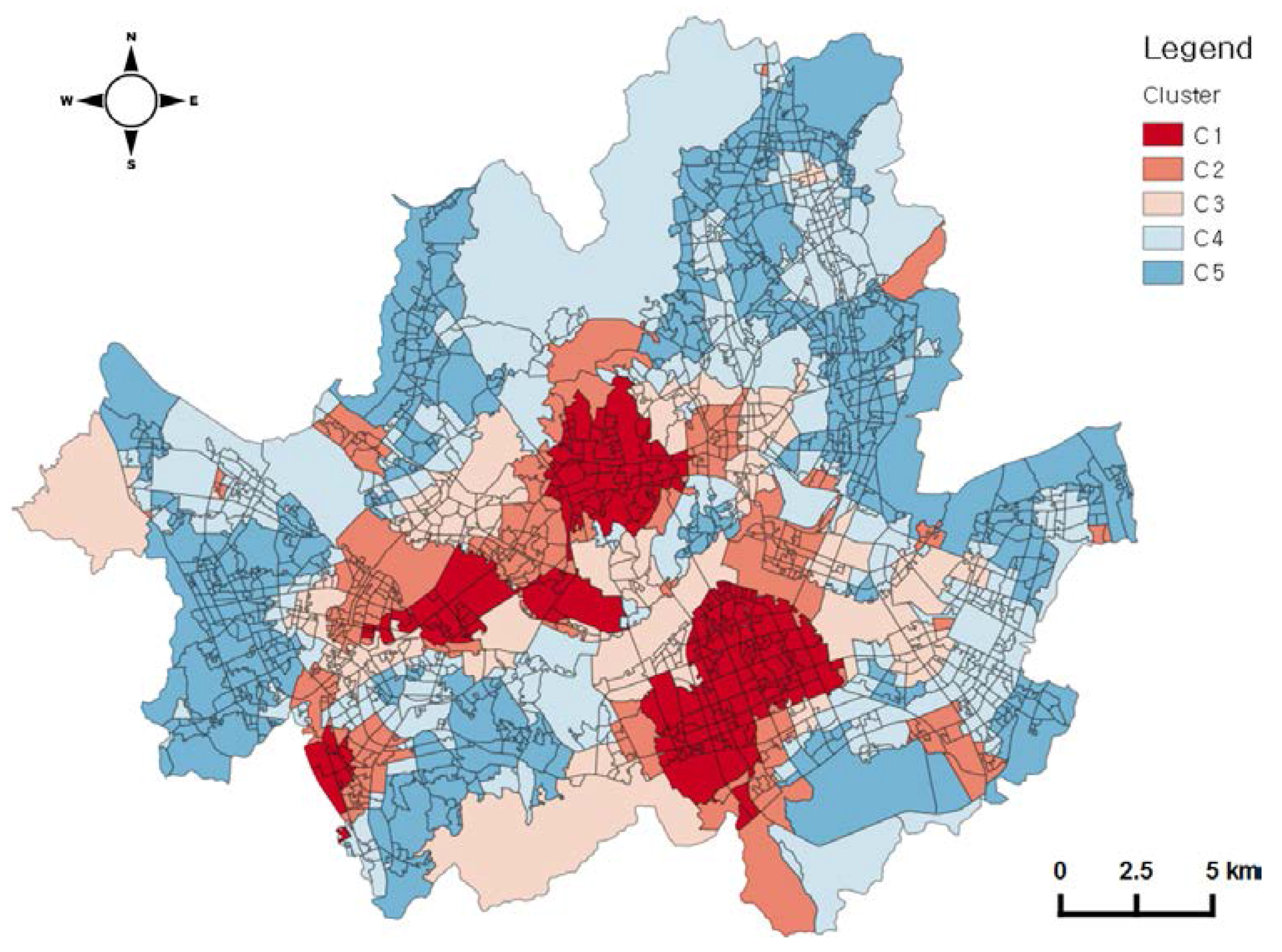
Through clustering, we could also obtain the spatial pattern of public-transport travel. The spatial distribution of clusters is shown in Figure 10. C1 contains the main central business district (CBD) and the major business districts, such as Gangnam and Yeoeuido. C2 and C3 are located beside C1 areas. C4 and C5 are located on the edge of the city. The spatial distribution of C1 is consistent with employment centers in Seoul in other research, which was undertaken by using statistical data only [48,49]. In addition, the spatial pattern of the clusters resembles the urban structure from the spatial restructuring plan developed by the Seoul Metropolitan Government [50]. This enables us to give meaning to our results and to explain the relationship between travel patterns and local environments; the spatial pattern of human mobility gives information on the influence of built-environment structures on travel patterns.
4.2. Relating Mobility Pattern with Local Environmental Characteristics
4.2.1. Descriptive Analysis
Table 3 shows the mean values of a set of socio-demographic, land-use and transportation characteristics of each identified cluster. C1 has the highest concentration of companies, more than two times that of the other clusters, and consequently the lowest population. C2 has the highest industrial area. C5 has the highest number of residents and the highest residential area. C5 also has the lowest commercial area and the lowest value of aging. C3 and C4 have the third and second highest population and almost half of their area is residential. An important difference between these two clusters is the concentration of companies. C3 also has the second highest number of businesses. In terms of transportation characteristics, C1 and C5 are characterized by a large number of public transportation users. C2 has the lowest passengers even though the population and residential area of C2 are higher than those of C1. Since C1 has more than twice the number of employees compared to C2, it can be considered that the number of employees has a large influence on the number of passengers. Besides, C2 has the smallest number of subway stations. It was observed that the number of public-transportation users is positively correlated to the number of subway stations.
Relating to the transportation characteristics, boarding around the morning peak appears to be a function of population and alighting around the morning peak is a function of the number of employees/businesses in the area. In addition, the average daily number of passengers appears to have a linear relationship with the summation of population and the number of employees except in C1. Excluding C1, the number of passengers has a positive linear relationship with the population and a negative linear relationship with the number of employees. C1 is the least populated region in Seoul, but there are a lot of passengers (movements); alighting and boarding throughout the area. Also, C1 has the largest number of stations although the total area of C1 is the smallest. It might be attributed to the highest number of businesses and employees in C1 among the clusters and concentration of public-transportation facilities. Meanwhile, travel in C1 during the weekend becomes like that in C3. C1 and C3 are closely located geographically as shown in Figure 10. It is thought that weekday patterns of C1 and C3 may vary significantly due to the large number of employees, but the difference of the weekend is reduced because of the low impact of commuting. C3 has the largest recreational facilities area and the least passenger gap between weekdays and the weekend. C4 and C5 are both primarily residential areas, but the ridership volume of C5 is higher than that of C4. Heavier residential density in C5 probably contributes to the number of passengers.
4.2.2. Selected Variables (Local Environments) Using PCA
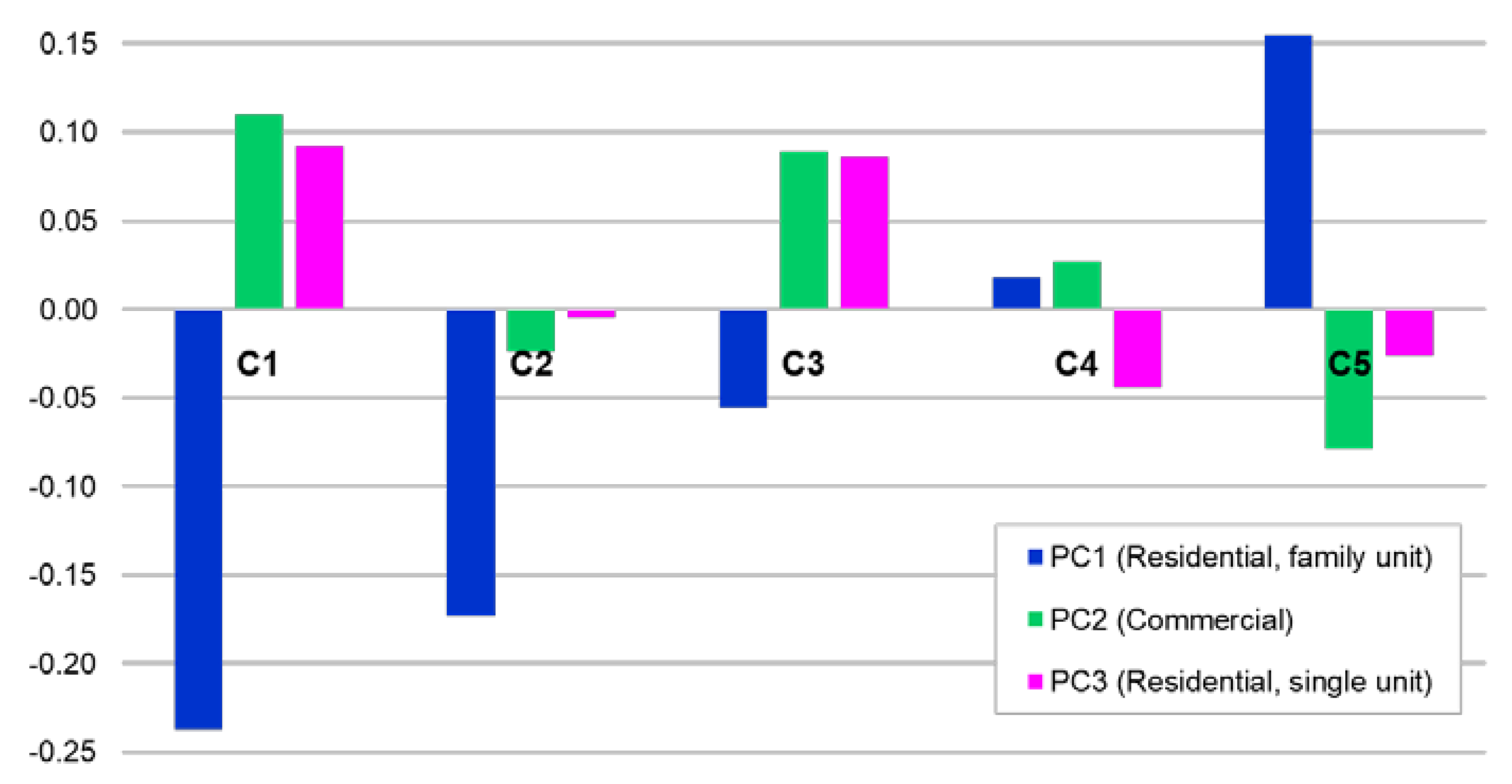
The local environment data set was reduced from 142 dimensions to only 3 by ignoring eigenvectors that have insignificant eigenvalues. Using the varimax rotation, three components were retained based on visual inspection of the scree plot. The three-component solution explains 53.69% of total variance. The first principal component (PC1) explains 40.18% of the total variance and is dominated by total population and number of households. The second principal component (PC2) that explains 9.69% of the total variance is influenced by the number of businesses, accommodation businesses, food services, etc. The third component (PC3) accounts for 3.81% of the total variance and is dominated by studio apartments, unrelated households, rooms for monthly rent, and single-member households. Based on these, three components could be considered as a residential function (family unit), commercial function, and residential function (single unit), respectively.
4.2.3. Relationship between Mobility Pattern and local Environments
For each cluster of the travel patterns, the average values of newly constructed variables: PC1, PC2, PC3, are plotted in Figure 11. With regard to the pattern of C1 areas, the residential function (family unit) component is the lowest and the commercial function component is higher than the other clusters. This indicates that these local environmental characteristics tend to attract people in the morning but drive them out in the evening. For C5, the residential function component is the highest and the commercial function component is the lowest in clusters, indicating that areas of C5 tend to be associated with residential-dominated areas rather than commercial areas. C2, C3, and C4 have moderate characteristics. Out of them, C3 has similar pattern with C1; negative PC1, positive PC2 and PC3. This is likely to be linked to the similar temporal pattern of C1 and C3 during the weekend, as discussed in previous section.
In order to further analyze the relationship between mobility patterns and environmental characteristics, a correspondence analysis is applied. We categorize each PC value into three, high, medium, and low, according to normalized values of the three components. The graph from the correspondence analysis, as shown in Figure 12, shows the relationship between the clusters identified by mobility patterns and local environmental characteristics. In the graph, trip patterns are represented by black rectangles, and socio-demographic variables are in various shapes. This shows that C1 is quite close to PC2-high, indicating that this area tends to be located in commercial areas. Both C2 and C3 are close to PC1-medium. But C3 is closer to PC3-high than the other clusters, indicating that C3 tends to have a residential function in single units such as one-person households. C5 is close to PC3-low, indicating that C5 has a family unit residential function. A visual inspection of the CA bi-plot revealed that the locations of trip patterns and local environmental variables show similarities between them.
5. Conclusions
This study aimed to identify the travel patterns from transit smart-card data and its association with local environmental characteristics. Previous studies have focused on explaining trip purpose and its relation with land-use type. In contrast, we found major travel patterns on a citywide level while simultaneously assessing the inter-relationships with local environmental characteristics. Using seven-day transit smart-card data in Seoul, we investigated the temporal and spatial patterns of boarding and alighting of public transportation, and identified the links between travel patterns and other local environmental factors in urban environments.
We found that the temporal pattern of urban mobility reflects the daily activities in the urban areas. The major travel patterns, classified in five clusters, are identified by utilizing K-SC clustering. From the five travel patterns, the main representative activities are well described. In case of C1, many people come in during the morning and move out in the evening and night. Meanwhile, C5 showed the opposite pattern. The result is strongly correlated with general daily routines. Moreover, each cluster showed its own distinctive pattern, which reflects the daily activity inside each cluster. Accordingly, the regional functions of the clusters can be estimated by travel patterns.
The spatial pattern of the five clusters is closely related to the urban function from other data sources; urban planning maps, and other research. We could identify from the spatial patterns of the clusters’ population tendency and urban regional function that C1 is located in the center of a city’s business district and C5 is located on the edge of a city and is a residential area. Furthermore, it was shown that the residential population, the number of employees and the number of stations are related to the public-transportation usage. Hence, when designing a new public-transportation facility, it is important to consider the factors such as population and existing transportation facilities in a comprehensive way. For instance, the C2 area in the case study area needs to be considered as a priority if new transportation facilities are to be built.
In conclusion, this study figured out that the clustered travel patterns were differentially related to environment variables. The consideration of socio-demographic characteristics from the census and land use information may be useful for identifying its own function in the region and estimating the relationships among travel patterns. The travel patterns on a citywide level can be used to understand the dynamics of the urban population that dominate a city. We can further evaluate this framework on other cities or countries in order to estimate the applicability of supporting the use of our approach to improve the understanding of urban mobility based on smart-card data sources.
Acknowledgments
We would like to thank the Transport Policy Division of the Seoul Metropolitan Government and related organizations for their help in making available various data including smart-card records and other information. This work was partially supported by a grant [MOIS-DP-2015-10] through the Disaster and Safety Management Institute funded by Ministry of the Interior and Safety of Korean government. The authors would also like to thank the anonymous reviewers for their valuable comments and suggestions to improve the quality of the paper.
Author Contributions
Mi-Kyeong Kim, Sangpil Kim, and Hong-Gyoo Sohn were responsible for the research design, data preparation, performance of experiments and results analysis. Mi-Kyeong Kim designed and implemented the approach and analyzed the results. Sangpil Kim contributed to data processing and result analysis. Mi-Kyeong Kim and Hong-Gyoo Sohn wrote the paper; Hong-Gyoo Sohn finally approved the published work.
Conflicts of Interest
The authors declare no conflict of interest.
References
- Frankhauser, P. From fractal urban pattern analysis to fractal urban planning concepts. In Computational Approaches for Urban Environments; Springer International Publishing: New York, NY, USA, 2015; pp. 13–48. [Google Scholar]
- Rodrigues da Silva, A.N.; Manzato, G.G.; Pereira, H.T.S. Defining functional urban regions in bahia, brazil, using roadway coverage and population density variables. J. Transp. Geogr. 2014, 36, 79–88. [Google Scholar] [CrossRef]
- Lin, T.; Sun, C.; Li, X.; Zhao, Q.; Zhang, G.; Ge, R.; Ye, H.; Huang, N.; Yin, K. Spatial pattern of urban functional landscapes along an urban–rural gradient: A case study in xiamen city, china. Int. J. Appl. Earth Obs. Geoinf. 2016, 46, 22–30. [Google Scholar] [CrossRef]
- Veneri, P. The identification of sub-centres in two italian metropolitan areas: A functional approach. Cities 2013, 31, 177–185. [Google Scholar] [CrossRef]
- Cats, O.; Wang, Q.; Zhao, Y. Identification and classification of public transport activity centres in stockholm using passenger flows data. J. Transp. Geogr. 2015, 48, 10–22. [Google Scholar] [CrossRef]
- Zhong, C.; Schläpfer, M.; Arisona, S.M.; Batty, M.; Ratti, C.; Schmitt, G. Revealing centrality in the spatial structure of cities from human activity patterns. Urban Stud. 2017, 54, 437–455. [Google Scholar] [CrossRef]
- Yuan, N.J.; Zheng, Y.; Xie, X.; Wang, Y.; Zheng, K.; Xiong, H. Discovering urban functional zones using latent activity trajectories. IEEE Trans. Knowl. Data Eng. 2015, 27, 712–725. [Google Scholar] [CrossRef]
- Toole, J.L.; Ulm, M.; González, M.C.; Bauer, D. Inferring land use from mobile phone activity. In Proceedings of the ACM SIGKDD International Conference on Knowledge Discovery and Data Mining, Beijing, China, 12–16 August 2012; pp. 1–8. [Google Scholar]
- Pan, H.; Shen, Q.; Zhang, M. Influence of urban form on travel behaviour in four neighbourhoods of shanghai. Urban Stud. 2009, 46, 275–294. [Google Scholar]
- Ganciu, A.; Balestrieri, M.; Imbroglini, C.; Toppetti, F. Dynamics of metropolitan landscapes and daily mobility flows in the italian context. An analysis based on the theory of graphs. Sustainability 2018, 10, 596. [Google Scholar] [CrossRef]
- Jiang, B.; Yao, X. Geospatial Analysis and Modelling of Urban Structure and Dynamics; Springer: Dordrecht, The Netherlands, 2010. [Google Scholar]
- Loidl, M.; Wallentin, G.; Cyganski, R.; Graser, A.; Scholz, J.; Haslauer, E. Gis and transport modeling—strengthening the spatial perspective. ISPRS Int. J. Geo-Inf. 2016, 5, 84. [Google Scholar] [CrossRef]
- Dominic, S. Relationships between land use, socioeconomic factors, and travel patterns in britain. Environ. Plan. B Plan. Des. 2001, 28, 499–528. [Google Scholar]
- Schwanen, T.; Dijst, M.; Dieleman, F.M. The Relationship between Land Use and Travel Patterns: Variations by Household Type; Utrecht University Repository: Utrecht, The Netherlands, 2005. [Google Scholar]
- Boarnet, M.G.; Crane, R. Travel by Design: The Influence of Urban Form on Travel; Oxford University Press on Demand: Oxford, UK, 2001. [Google Scholar]
- Milakis, D.; Efthymiou, D.; Antoniou, C. Built environment, travel attitudes and travel behaviour: Quasi-longitudinal analysis of links in the case of greeks relocating from us to Greece. Sustainability 2017, 9, 1774. [Google Scholar] [CrossRef]
- Handy, S. Methodologies for exploring the link between urban form and travel behavior. Transp. Res. Part D Transp. Environ. 1996, 1, 151–165. [Google Scholar] [CrossRef]
- Jen-Jia, L.; An-Tsei, Y. Structural analysis of how urban form impacts travel demand: Evidence from Taipei. Urban Stud. 2009, 46, 1951–1967. [Google Scholar]
- Calabrese, F.; Diao, M.; Di Lorenzo, G.; Ferreira, J.; Ratti, C. Understanding individual mobility patterns from urban sensing data: A mobile phone trace example. Transp. Res. Part C Emerg. Technol. 2013, 26, 301–313. [Google Scholar] [CrossRef]
- Ma, X.; Wu, Y.-J.; Wang, Y.; Chen, F.; Liu, J. Mining smart card data for transit riders’ travel patterns. Transp. Res. Part C Emerg. Technol. 2013, 36, 1–12. [Google Scholar] [CrossRef]
- Goulet-Langlois, G.; Koutsopoulos, H.N.; Zhao, J. Inferring patterns in the multi-week activity sequences of public transport users. Transp. Res. Part C Emerg. Technol. 2016, 64, 1–16. [Google Scholar] [CrossRef]
- Roth, C.; Kang, S.M.; Batty, M.; Barthélemy, M. Structure of urban movements: Polycentric activity and entangled hierarchical flows. PLoS ONE 2011, 6, e15923. [Google Scholar] [CrossRef] [PubMed]
- Seoul Metropolitan Government. Seoul Public Transportation Story by Numbers; Transportation Policy Department, Seoul Metropolitan Government: Seoul, Korea, 2014.
- Seoul Solution. Establishing Transportation Card System. Available online: https://seoulsolution.kr/ko/content/%EA%B5%90%ED%86%B5%EC%B9%B4%EB%93%9C%EC%8B%9C%EC%8A%A4%ED%85%9C-%EA%B5%AC%EC%B6%95 (accessed on 9 September 2017).
- MOI. Resident Registration Data. Available online: http://rcps.egov.go.kr:8081/jsp/stat/ppl_stat_jf.jsp (accessed on 18 May 2016).
- Seoul Statistics. Transportation Modes of Seoul Citizen. Available online: http://stat.seoul.go.kr/jsp3/stat.db.jsp (accessed on 18 May 2016).
- SGIS. Explanation of Term. Available online: http://211.34.86.29/contents/support/support_04.jsp (accessed on 7 November 2017).
- Jeon, J. Demarcation of Statistical Area. Available online: http://kostat.go.kr/portal/korea/kor_nw/2/14/1/index.board?bmode=read&aSeq=56336 (accessed on 18 May 2016).
- Cockings, S.; Martin, D. Zone design for environment and health studies using pre-aggregated data. Soc. Sci. Med. 2005, 60, 2729–2742. [Google Scholar] [CrossRef] [PubMed]
- Yuan, N.J.; Zheng, Y.; Xie, X. Segmentation of Urban Areas Using Road Networks; Technical Report MSR-TR-2012-65; Microsoft: Albuquerque, NM, USA, 2012. [Google Scholar]
- Langford, M. An evaluation of small area population estimation techniques using open access ancillary data. Geogr. Anal. 2013, 45, 324–344. [Google Scholar] [CrossRef]
- Xie, Y. The overlaid network algorithms for areal interpolation problem. Comput. Environ. Urban Syst. 1995, 19, 287–306. [Google Scholar] [CrossRef]
- Lee, K. Impacts of neighborhood’s land use and transit accessibility on residents’ commuting trips—A case study of seoul. J. Korea Acad.-Ind. Coop. Soc. 2013, 14, 4593–4601. [Google Scholar] [CrossRef]
- City Planning Department. Seoul Metropolitan City Planning Decree; Seoul Metropolitan Government: Seoul, Korea, 2018; Volume 6776.
- Wang, H.; Wang, W.; Yang, J.; Yu, P.S. Clustering by pattern similarity in large data sets. In Proceedings of the ACM SIGMOD International Conference on Management of Data, Madison, Wisconsin, 3–6 June 2002; Moon, M.F.B., Ailamaki, A., Eds.; pp. 394–405. [Google Scholar]
- Kriegel, H.-P.; Kröger, P.; Zimek, A. Clustering high-dimensional data: A survey on subspace clustering, pattern-based clustering, and correlation clustering. ACM Trans. Knowl. Discov. Data 2009, 3, 1–58. [Google Scholar] [CrossRef]
- Gonzalez, M.C.; Hidalgo, C.A.; Barabasi, A.L. Understanding individual human mobility patterns. Nature 2008, 453, 779–782. [Google Scholar] [CrossRef] [PubMed]
- Yang, J.; Leskovec, J. Patterns of temporal variation in online media. In Proceedings of the 4th ACM International Conference on Web Search and Data Mining, Hong Kong, China, 9–12 February 2011; pp. 177–186. [Google Scholar]
- Caliński, T.; Harabasza, J. A dendrite method for cluster analysis. Commun. Stat.-Theory Methods 1974, 3, 1–27. [Google Scholar] [CrossRef]
- Hartigan, J.A. Clustering Algorithms; John Wiley & Sons, Inc.: New York, NY, USA, 1975. [Google Scholar]
- Kaufman, L.; Rousseeuw, P.J. Finding Groups in Data: An Introduction to Cluster Analysis; John Wiley & Sons: New York, NY, USA, 2009. [Google Scholar]
- Xie, X.L.; Beni, G. A validity measure for fuzzy clustering. IEEE Trans. Pattern Anal. Mach. Intell. 1991, 13, 841–847. [Google Scholar] [CrossRef]
- Rousseeuw, P.J. Silhouettes: A graphical aid to the interpretation and validation of cluster analysis. J. Comput. Appl. Math. 1987, 20, 53–65. [Google Scholar] [CrossRef]
- Sugar, C.A.; James, G.M. Finding the number of clusters in a dataset: An information-theoretic approach. J. Am. Stat. Assoc. 2003, 98, 750–763. [Google Scholar] [CrossRef]
- Wang, F. Quantitative Methods and Applications in Gis; CRC Press: Boca Raton, FL, USA, 2006. [Google Scholar]
- Abdi, H.; Valentin, D. Multiple correspondence analysis. In Encyclopedia of Measurement and Statistics; SAGE Publications: Thousand Oaks, CA, USA, 2007; pp. 651–657. [Google Scholar]
- Guo, Y. Knowledge Discovery for Design Optimization Using Correspondence Analysis; Simon Fraser University: Burnaby, BC, Canada, 2015. [Google Scholar]
- Jun, M.J.; Choi, S.; Wen, F.; Kwon, K.H. Effects of urban spatial structure on level of excess commutes: A comparison between seoul and los angeles. Urban Stud. 2018, 55, 195–211. [Google Scholar] [CrossRef]
- Kim, J.I.; Yeo, C.H.; Kwon, J.-H. Spatial change in urban employment distribution in seoul metropolitan city: Clustering, dispersion and general dispersion. Int. J. Urban Sci. 2014, 18, 355–372. [Google Scholar] [CrossRef]
- Koo, H.; Lee, B.; Lee, C.S. Analysis of changes in spatial structure of seoul by analyzing the land price changes of station influence areas. J. Korean Soc. Surv. Geodesy Photogramm. Cartogr. 2016, 34, 63–70. [Google Scholar] [CrossRef]
Figure 1.
Administrative districts (gu) of Seoul.

Figure 2.
Newly constructed unit area of the study.

Figure 3.
Schematic diagram of the research flow.

Figure 4.
Point data containing ridership (a) and the results of ridership distribution along the streets (b).
Figure 4.
Point data containing ridership (a) and the results of ridership distribution along the streets (b).
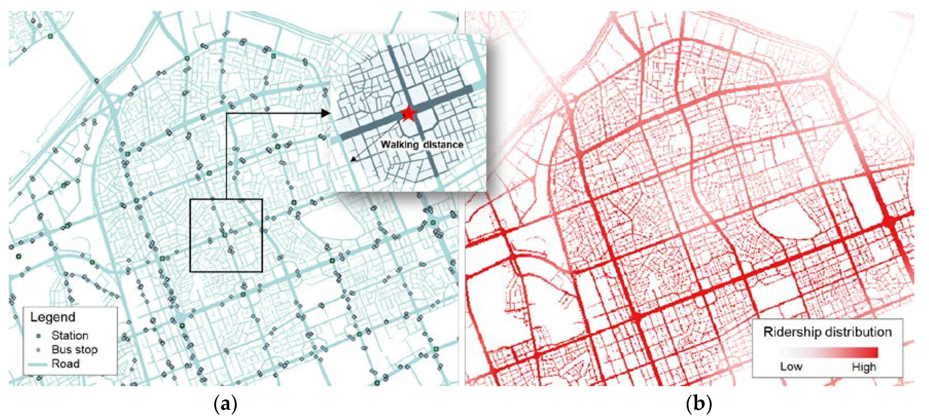
Figure 5.
Validity measures as a function of the number of clusters.

Figure 6.
Temporal pattern during a week (total counts of boarding and alighting).

Figure 7.
Pearson’s correlation coefficients of daily temporal patterns.

Figure 8.
Weekday pattern of boarding (a) and alighting (b).

Figure 9.
Weekend pattern of boarding (a); alighting (b).
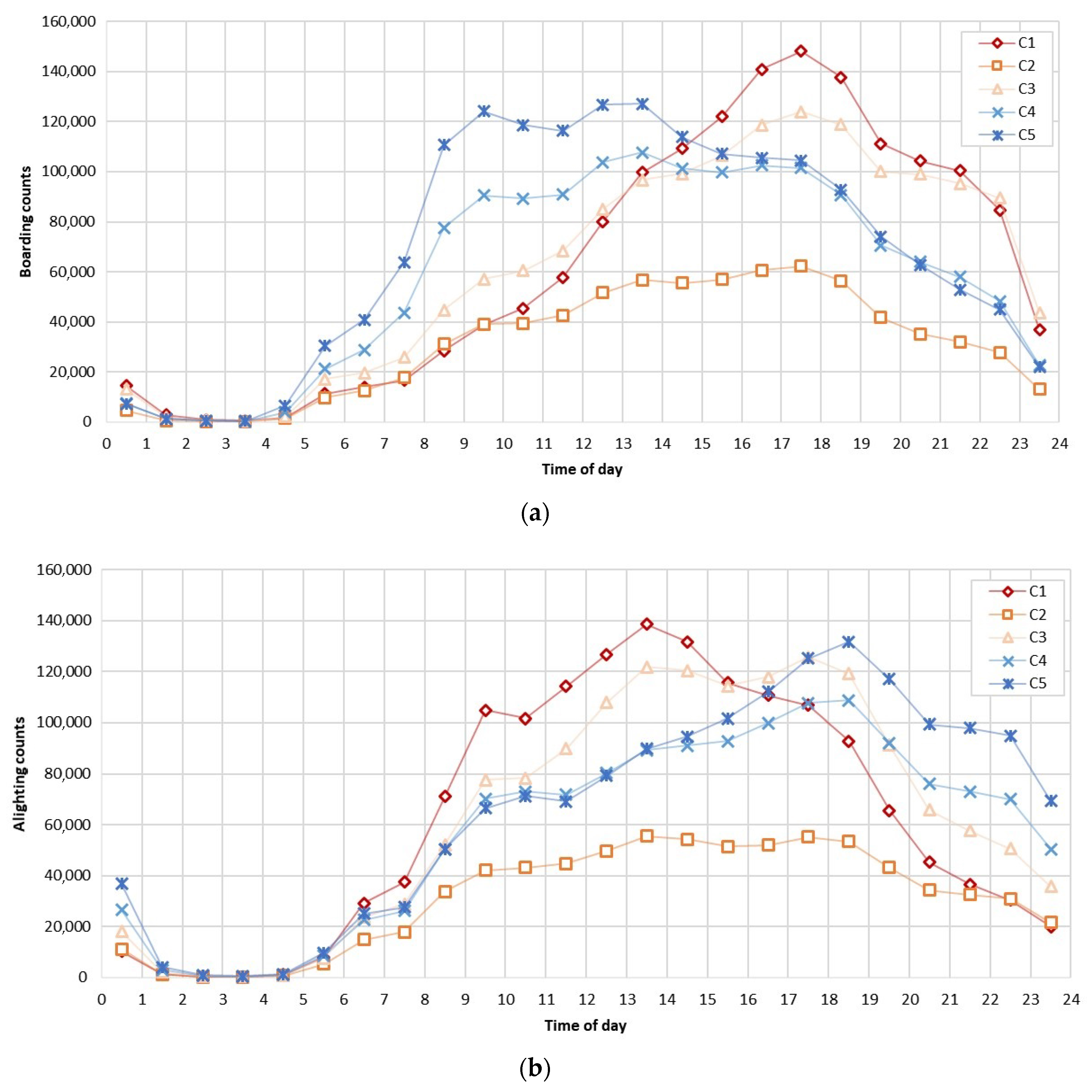
Figure 10.
Spatial distribution of clusters (spatial pattern of mobility).

Figure 11.
Average of newly constructed variables for five clusters.

Figure 12.
Relationship between mobility patterns and environments.


Table 1.
The configuration of arranged data from transit records.
| Transaction Number | Boarding Time (yyyy/mm/dd/hh/mm/ss) | ID of Boarding Location | Alighting Time (yyyy/mm/dd/hh/mm/ss) | ID of Alighting Location | Number of Passengers |
|---|---|---|---|---|---|
| 1 | 20150318092455 | 4196066 | 20150318092714 | 4196117 | 1 |
| 2 | 20150318214734 | 4196061 | 20150318215035 | 4196065 | 1 |
| 3 | 20150318225205 | 12174 | 20150318225855 | 8001017 | 1 |
| 4 | 20150318075726 | 70647 | 20150318082805 | 10585 | 1 |
| 5 | 20150318070948 | 216 | 20150318084718 | 4101317 | 1 |
| … | … | … | … | … | … |
Table 2.
Local environment data.
| Category | Description | Variables |
|---|---|---|
| Population | Age/sex distribution | in_age_001~054 |
| Education level (type of last school completed) | in_edu_001~008 | |
| Marital status | in_wed_001~008 | |
| Household | Number of rooms | ga_co_001~011 |
| Type of occupancy | ga_po_001~006 | |
| Family type of household | ga_sd_001~006 | |
| Housing | Floor space of house | ho_ar_001~009 |
| Type of housing | ho_gb_001~006 | |
| Construction year | ho_yr_001~013 | |
| Business | Number of businesses by 9th industrial classification in Korea | cp9_bnu_01~18 |
| Number of employees by 9th industrial classification in Korea | cp9_bem_01~18 | |
| Land use/Land cover | Residential area | lcm_110 |
| Industrial area | lcm_120 | |
| Commercial area | lcm_130 | |
| Recreational facilities | lcm_140 | |
| Roads | lcm_150 | |
| Public facilities | lcm_160 | |
| Agricultural area | lcm_200 | |
| Forest | lcm_300 | |
| Grass | lcm_400 | |
| Wetland | lcm_500 | |
| Bare land | lcm_600 | |
| Water | lcm_700 |
Table 3.
Descriptive characteristics of clusters.
| Major Variables | C1 | C2 | C3 | C4 | C5 |
|---|---|---|---|---|---|
| Socio-demographic characteristics | |||||
| Population | 2263 | 3209 | 4376 | 4512 | 5241 |
| Aging index * | 158 | 97 | 106 | 84 | 77 |
| Youth dependency ratio ** | 14 | 18 | 17 | 19 | 20 |
| Number of households | 943 | 1210 | 1702 | 1629 | 1878 |
| Number of houses | 613 | 849 | 1070 | 1199 | 1318 |
| Number of businesses | 753 | 313 | 347 | 231 | 224 |
| Number of employees | 6494 | 2226 | 2212 | 1225 | 853 |
| Land-use (LU) characteristics | |||||
| Residential area (%) | 29.46 | 36.61 | 43.42 | 47.87 | 55.90 |
| Industrial area (%) | 0.75 | 2.61 | 0.60 | 0.21 | 0.24 |
| Commercial area (%) | 36.02 | 25.64 | 21.20 | 15.27 | 14.06 |
| Recreational facilities area (%) | 0.52 | 0.65 | 0.93 | 0.52 | 0.48 |
| Roads (%) | 20.05 | 19.91 | 19.61 | 18.09 | 15.74 |
| Total area (km2) | 55.67 | 72.77 | 100.17 | 191.33 | 189.14 |
| Transportation characteristics | |||||
| Number of subway stations | 86 | 57 | 67 | 85 | 72 |
| Number of bus stops | 1424 | 1659 | 1757 | 3557 | 5096 |
| The average daily number of passengers (weekday) | 4,644,463 | 2,327,482 | 3,454,941 | 3,866,049 | 4,442,733 |
| The average daily number of passengers (weekend) | 3,010,399 | 1,501,063 | 2,997,360 | 2,814,313 | 3,232,683 |
| Boardings around the morning peak | 39,787 | 54,128 | 84,149 | 149,850 | 211,048 |
| Boardings around the evening peak | 210,410 | 85,978 | 108,961 | 102,927 | 97,835 |
| Alightings around the morning peak | 251,609 | 98,525 | 103,778 | 99,425 | 85,157 |
| Alightings around the evening peak | 93,492 | 59,103 | 104,576 | 120,964 | 157,452 |
* Aging index: the population aged 65 or over per 100 population aged 0 to 14; ** youth dependency ratio: the population aged 0 to 14 over per 100 population aged 15 to 64.
© 2018 by the authors. Licensee MDPI, Basel, Switzerland. This article is an open access article distributed under the terms and conditions of the Creative Commons Attribution (CC BY) license (http://creativecommons.org/licenses/by/4.0/).
Share and Cite
MDPI and ACS Style
Kim, M.-K.; Kim, S.; Sohn, H.-G. Relationship between Spatio-Temporal Travel Patterns Derived from Smart-Card Data and Local Environmental Characteristics of Seoul, Korea. Sustainability 2018, 10, 787. https://doi.org/10.3390/su10030787
AMA Style
Kim M-K, Kim S, Sohn H-G. Relationship between Spatio-Temporal Travel Patterns Derived from Smart-Card Data and Local Environmental Characteristics of Seoul, Korea. Sustainability. 2018; 10(3):787. https://doi.org/10.3390/su10030787
Chicago/Turabian StyleKim, Mi-Kyeong, Sangpil Kim, and Hong-Gyoo Sohn. 2018. "Relationship between Spatio-Temporal Travel Patterns Derived from Smart-Card Data and Local Environmental Characteristics of Seoul, Korea" Sustainability 10, no. 3: 787. https://doi.org/10.3390/su10030787
Note that from the first issue of 2016, this journal uses article numbers instead of page numbers. See further details here.