Improving the Forecasting Accuracy of Crude Oil Prices

Abstract

Currently, oil is the key element of energy sustainability, and its prices and economy have a strong mutual influence. Modeling a good method to accurately predict oil prices over long future horizons is challenging and of great interest to investors and policymakers. This paper forecasts oil prices using many predictor variables with a new time-varying weight combination approach. In doing so, we first use five single-variable time-varying parameter models to predict crude oil prices separately. Second, every special model is assigned a time-varying weight by the new combination approach. Finally, the forecasting results of oil prices are calculated. The results show that the paper’s method is robust and performs well compared to random walk.

1. Introduction

The sustainable development of energy has a huge influence on regional stability and economic growth [1]. Governments regulate relevant policies to drive the energy sustainability, but it usually takes a long time from the formulation of a policy to its implementation. For example, a new energy law transposed the European Union third energy package and energy development strategy of Serbia by 2025, with projections to 2030, and it was up to five years [2]. Although many policies advocate for the use of renewable energy, oil is still the main fuel in the current world (in the first quarter of 2017, the total consumption of OECD liquid fuels was 46.78 million barrels per day—data from the U.S. Energy Information Administration, https://www.eia.gov/outlooks/steo/tables/pdf/3dtab.pdf). Moreover, oil prices could lead to the implementation of policies. For example, interest in energy-related policy was revived with the high oil prices in the late 2000s, and the composition of governmental supports across sectors shifted tectonically with the American Recovery and Reinvestment Act, away from fossil fuels and toward unprecedented levels of support for renewable energy [3]. Therefore, accurate price forecasting of oil could provide some valuable information for making policies and relieve the time-lag problems of polices.

The volatility of oil prices is affected by many issues, including supply and demand, the futures market, and political stability and geopolitics. Hamilton (2009) documented that the causes of the different volatility were differences in supply and demand [4]. Hamilton found that previous oil price shocks were primarily caused by physical disruptions in supply, whereas the price run-up of 2007–2008 was caused by strong demand. Huang (2017) studied the world economy, oil stocks, futures market, and political stability in the Middle East with regard to oil price fluctuations in multiple time horizons [5]. Huang found that these factors have some influence on the volatility of oil prices in one or more horizons. In contrast, oil shocks have a great impact on the economy. Hamilton (1983) supported the idea that oil shocks were a contributing factor to at least some of the U.S. recessions prior to 1972 [6]. Wong and El (2017) suggested the need for more economic diversification at the country level in the Gulf Corporation Council region to mitigate high volatility in the event of oil shocks [7]. Hence, an accurate forecast of oil prices is of great interest to investors and policymakers, and it is a big challenge for researchers. This paper proposes a new time-varying weight combination approach.

Recently, there have been two main methods for predicting the price of oil. One method is based on dynamic model averaging (DMA). In 2010, Raftery et al. [8] developed the DMA model to predict the output strip thickness for a cold rolling mill, and Koop and Korobilis (2012) applied it to an economic variable’s forecast [9]. For oil forecasting, Drachal (2016), Naser (2016), and Wang et al. (2015) used the DMA model predict different class of oil prices [10,11,12]. The superiority of the DMA model not only captures the time-varying property of the variables, but could also select the optimum model automatically. However, this method will meet the curse of dimensionality when the predictor variables are larger. The other method is to model the combination method. In 2015, Baumeister and Kilian [13] proposed a forecast combination approach with inverse recursive mean-squared prediction error (MSPE). (Manescu and Van Robays (2016) utilized this method to predict real Brent oil prices [14]). Their method significantly improved the accuracy with a combination of six models: a vector autoregression model of the global oil market, a forecast based on the price of non-oil industrial raw materials, a no-change forecast, a forecast based on oil futures prices, the spread between the spot prices of gasoline and crude oil, and the time-varying parameter model of the gasoline and heating oil spreads. However, the increases in the MPSE with the different models may contribute to overlooking the truth that the different models themselves may lead to differences. To overcome these, all the models that we use have the same single-variable time-varying parameter to fit the data.

In this paper, we follow Baumeister and Kilian’s [13] idea and propose a new time-varying weight combination method with some special dependence (this method is similar to Kendall’s tau and Spearman’s rho). The capture of this special dependence is carried concordantly between the predictor variable and the oil prices. Additionally, the weight is built on the assumption that the dependence is stronger and the weight is higher, and vice versa. The steps for constructing the model are portrayed below. First, we used five single-variable time-varying parameter models to predict the crude oil prices separately. These variables were oil production, oil inventory, the Kilian’s index, non-energy commodity prices, and crack spread selected from four aspects supply, demand, non-energy, and energy-related. Second, every special model was assigned a time-varying weight by the new combination approach. Finally, the forecasting results of the oil prices were calculated. Our method, compared to random walk (here we follow Alquist and Kilian (2010) and treat the random walk as the benchmark for comparison purposes [15]). behaves better in terms of accuracy. Furthermore, our method is robust compared to the inverse recursive MPSE weight method.

This paper makes two main contributions. The first is to build five single-variable time-varying parameter models related to the four significant impacts of oil prices. The second is to propose a new time-varying weight combination method. This method behaves better with regard to improving the accuracy of forecasts. The remainder of the paper is designed as follows. In Section 2, we introduce the methodology of time-varying combination. The data selection and empirical results are introduced in Section 3. Section 4 shows the discussion and conclusions.

2. Methodology

In this subsection, we first introduce the general time-varying parameter (TVP) model and Kalman filter (Kim and Nelson 1999 [16]). Next, a single-variable TVP model is provided. Finally, following the single-variable TVP model, a time-varying weight method is proposed.

TVP models: Consider the following regression model in which the regression coefficients are time-varying with specific dynamics:

$$y_t=x_t{\beta }_t+{ϵ}_t,$$

$${\beta }_t=\mu +F{\beta }_{t-1}+{\eta }_t,$$

where t is time; ${ϵ}_{t}i.i.d.N(0,R)$; ${\eta }_{t}i.i.d.N(0,Q)$; $y_t$ is a $1\times 1$ dependent variable; $x_t$ is a $1\times k$ vector of independent or exogenous variables (k is constant). We assume that ${\beta }_t$ is $k\times 1$ dimension and $cov({ϵ}_t,{\eta }_t)=0$, so Q is a $k\times k$ matrix and F is a $k\times k$ matrix.

Kalman filter: The Kalman filter is described by the following six equations:

Prediction:

$${\beta }_{t|t-1}=\mu +F{\beta }_{t-1|t-1},$$

$$P_{t|t-1}=F{P}_{t-1|t-1}{F}^{\prime }+Q,$$

$${\eta }_{t|t-1}=y_t-y_{t|t-1}=y_t-x_t{\beta }_{t-1|t-1},$$

$$f_{t|t-1}=x_t{P}_{t-1|t-1}{z}_t^{\prime }+R,$$

Updating:

$${\beta }_{t|t}={\beta }_{t|t-1}+K_t{\eta }_{t|t-1},$$

$$P_{t|t}=P_{t|t-1}+K_t{x}_t{P}_{t|t-1},$$

where $K_t=P_{t|t-1}{X}_t^{\prime }{f}_{t|t-1}^{-1}$ is the Kalman gain, which determines the weight assigned to new information about ${\beta }_t$ contained in the prediction error. $P_{t|t}=E\left[({\beta }_t-{\beta }_{t|t-1}){({\beta }_t-{\beta }_{t|t-1})}^{\prime }\right]$ is the covariance matrix of ${\beta }_t$ conditional on information up to $t-1$ and $f_{t|t-1}=E\left[{\eta }_{t|t-1}^2\right]$.

Single-variable TVP model and time-varying weight methods: Assume that $x_t$ is a vector that only includes itself and its lag terms. Let $\mu$ and F be 0 and 1, respectively. The single-variable TVP model transforms as

$$y_t=x_t{\beta }_t+{ϵ}_t,$$

$${\beta }_t={\beta }_{t-1}+{\eta }_t.$$

The single-variable TVP model is estimated with a Gibbs sample algorithm (in oil price forecasting, Baumeister et al. (2013) used product spreads to forecast with this method [17]). (see Kim and Nelson 1999 [16]).

Based on the prediction results of all the single-factor TVP models, the time-varying weight combination approach is presented below. Let $x_t$ and $y_t$ be two time series. ${\Delta }_i$ is i orders difference operator, namely ${\Delta }_i{x}_t=x_t-x_{t-i}$, ${\Delta }_i{y}_t=y_t-y_{t-i}$. Define a score function $\delta$,

$$\delta ({\Delta }_i{x}_t,{\Delta }_i{y}_t)=\left\{\begin{array}{cc}1\hfill & {\Delta }_i{x}_t\ge 0\mathrm{and}{\Delta }_i{y}_t\ge 0\mathrm{or}{\Delta }_i{x}_t<0\mathrm{and}{\Delta }_i{y}_t<0,\hfill \\ 0\hfill & \mathrm{others}.\hfill \end{array}\right.$$

Then, let

$$M_{n,i,t}=\sum _{j=t-n+1}^t{\alpha }_j{\delta }_{i,j},$$

where n is the length of the rolling window and ${\alpha }_j$ is the dynamic value: ${\alpha }_j=c\ast (n-t-j)$, c is a positive constant, which means that we give a different weight for score function by the distance to t. Moreover, the closer to time t it is, the larger the score gets. This is based on the assumption that the current situation has a greater effect than usual. We also assume that it has m single-variable models to forecast the dependent variable $y_t$. Let these single variables be $x_{k,t}$, $k=1,2,\dots ,m$. We gain the j-th single-variable model with weight $w_k$,

$$w_k=\frac{M_{k,n,i,t}}{{\sum }_{k=1}^m{M}_{k,n,i,t}}.$$

Thus, the weight of every single-variable model has a dynamic weight.

3. Empirical Results and Robustness Test

The real price of crude oil—the dependent variable—is the focus of our paper. We consider the West Texas Intermediate crude oil prices (WTI) as a proxy for crude oil. Recently, Alquist and Kilian (2010) [15], Alquist et al. (2013) [18], Baumeister et al. (2013, 2014, 2015) [13,17,19], Wang et al. (2015) [12], Xiong et al. (2013) [20], Yin and Yang (2016) [21], Drachal (2016) [10] and Naser (2016) [11] all regarded WTI as a proxy variable for oil prices. We selected four factors: supply, demand, crack spread, and non-energy commodity prices. According to economic theory, supply and demand are the key factors for changing the price of a commodity. Therefore, many researchers employ it as an independent variable to forecast oil prices (Baumeister and Kilian (2012) [22], Fattouh et al. (2013) [23], Hamilton (2009) [4], Wang et al. (2015) [12], Baumeister et al. (2013, 2014, 2015) [13,17,19]), and we follow in their steps. For supply, two factors—oil production and oil inventory—were selected. Oil production and oil inventory reflect the increment and stock of oil prices, respectively, and oil production is a key influencing factor for oil prices because it is directly related to the supply of oil. The oil inventory signals the speculation, and its fluctuation easily bursts the volatility of oil prices. Kilian’s index is a proxy of demand introduced by Kilian (2009) [24], and is based on the percentage change of growth rates obtained from a panel of single-voyage bulk dry cargo ocean shipping freight rates measured in dollars per metric ton. This index can reflect the global demand of industrial commodities. Since industrial commodities rely primarily on oil, Kilian’s index should be a reasonable and suitable proxy for oil demand. The cost of oil refining technology has a direct impact on oil prices. In general, refined products follow an approximately fixed proportion of 3:2:1, which means obtaining two barrels of gasoline and one barrel of heating oil from three barrels of crude oil. We denote the price changes of the refining process as the crack spread. In commodity markets, energy and non-energy commodity prices are always somewhat interdependent because both of them are necessities in life. We treat non-energy commodity prices as another variable to forecast. The data of the WTI, oil production, oil inventory, and crack spread are all from the U.S. Energy Information Administration (EIA), and the non-energy commodity prices are collected from the World Bank. Kilian’s index comes from his personal webpage (http://www-personal.umich.edu/~lkilian/). In this paper, all the variables on prices are divided by the Consumer Price Index (CPI), and we follow Drachal (2016) [10] and consider the U.S. Consumer Price Index (https://fred.stlouisfed.org/series/CPIAUCSL) a proxy variable for global CPI. In addition, for all variables, we chose the monthly data from June 1986 to December 2016, for a total of 367 observations.

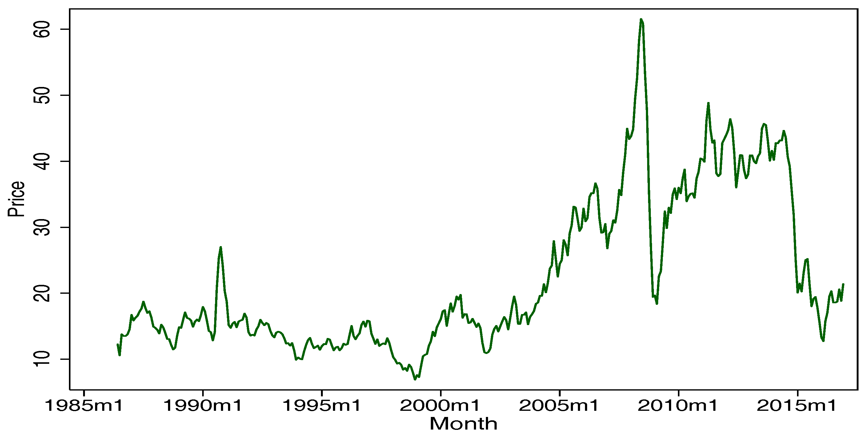
Before the forecasting, it was necessary to test the stationarity of the WTI. Figure 1 gives the real price of the WTI from June 1986 to December 2016, divided by the U.S. CPI. In

Table 1. Stationary and autoregressive conditional heteroskedasticity effect test.

	ADF Statistic	KPSS Statistic	PP Statistic
WTI	−2.369 (0.421)	4.269 (0.010)	−17.012 (0.158)
WTI-1	−7.596 (0.010)	0.053 (0.100)	−261.662 (0.010)
WTI-3	−6.496 (0.010)	0.068 (0.100)	−92.599 (0.010)
WTI-6	−5.279 (0.010)	0.102 (0.100)	−76.516 (0.010)
WTI-9	−6.804 (0.010)	0.150 (0.100)	−51.468 (0.010)
WTI-12	−5.403 (0.010)	0.230 (0.100)	−40.629 (0.010)
WTI-15	−4.261 (0.010)	0.292 (0.100)	−37.995 (0.010)
WTI-18	−3.631 (0.030)	0.363 (0.093)	−31.039 (0.010)
WTI-21	−3.897 (0.015)	0.422 (0.068)	−25.842 (0.020)
WTI-24	−3.133 (0.100)	0.492 (0.043)	−25.087 (0.023)

Note: The WTI is the real value of oil prices and WTI-x (x = {1, 3, 6, 9, 12, 15, 18, 21, 24}) denotes the first-order difference with a gap of x. (For example: Δ_xWTI_t = WTI_t − WTI_t−x, t is time). The values in the parentheses are p-values. ADF: augmented Dickey–Fuller; KPSS: Kwiatkowski–Phillips–Schmidt–Shin; PP: Phillips–Perron.

, the results of the augmented Dickey–Fuller (ADF) test and Phillips–Perron (PP) test both show that a unit root null hypothesis was refused except for the WTI. The Kwiatkowski–Phillips–Schmidt–Shin (KPSS) test also achieved the same results. Therefore, all the WTI differences remained stable, except the WTI demonstrated non-stationarity overall (the methods to test stationarity are various; this paper follows Drachal (2016) [10] and chooses the ADF, KPSS, and PP tests). Additionally, we selected the first 27 draws as prior data sets, the middle 240 as training sets, and the last 100 as the out-of-sample forecast. By 2000, repeating the Gibbs sample algorithms we gained the coefficients and variance, which discarded the first 500 draws and saved the last 1500.

Next, looking at the individual model: $y_{i,t+h}=y_{i,t}exp\left({\beta }_{i,t}{x}_{i,t}\right)$, i is the alternative model: global economic activity, crack spread, non-energy commodity prices, oil production, and oil inventory. In

Table 2. Success ratio compared to random walk.

Horizons	Models
	GEA	CS	NECI	OP	OI
1	47	46	44	56	51
3	48	56	48	56	53
6	46	49	52	52	42
9	48	51	55	41	48
12	49	51	57	45	50
15	45	53	57	61	57
18	48	58	61	58	51
21	51	53	50	58	45
24	47	52	52	56	50

Note: Here GEA, CS, NECI, OP and OI are the abbreviations of global economic activity proxy by the Kilian’s index, crack spread, non-energy commodity prices, oil production and oil inventory, respectively. The value in the table is the number of success ratios when compared with random walk. The bold shows that it is better than random walk—i.e., a value of no less than 50.

, compared to random walk, the fitting results for the success ratio are given (the success ratio equals the length of out-of-sample divided by the times of the specified model defeating random walk in out-of-sample forecasting [15]). Global economic activity presents poor prediction results, except for the horizon 21, with value 51. The model’s crack spread and non-energy commodity prices were optimal compared to random walk in most horizons. There were only two shorter horizons—1 and 6—in terms of crack spread, whereas 1 and 3 in non-energy prices did not exceed 50. In contrast, for oil production, getting rid of two mid-horizons—9 and 12—that were below 50, performed well in other horizons. The last single TVP model, oil inventory, performed normally and had three horizons that were below 50: 6, 9, and 21.

For the MSPE,

Table 3. Mean-squared prediction error (MSPE) compared to random walk.

Horizons	Models
	GEA	CS	NECI	OP	OI
1	$1.0037$ *	1.0143	0.8586	1.0020	0.9946
3	0.9855	0.9987	$\mathbf{0.8575}$ **	0.9995	0.9977
6	$\mathbf{0.9925}$ *	1.0016	$\mathbf{0.9459}$ *	0.9986	0.9987
9	$\mathbf{0.9962}$ **	1.0013	0.9987	1.0017	1.0020
12	0.9964	1.0002	1.0010	1.0004	1.0005
15	1.0069	1.0004	0.9992	0.9972	0.9962
18	1.0075	0.9953	0.9964	0.9970	0.9888
21	$1.0176$ **	0.9997	0.9966	0.9964	1.0052
24	$1.0232$ **	1.0005	0.9941	0.9976	1.0005

Note: Here GEA, CS, NECI, OP and OI are the abbreviations of global economic activity proxy according to the Kilian’s index, crack spread, non-energy commodity prices, oil production and oil inventory, respectively. The value in the table is calculated by the mean squared prediction error (MSPE) of random walk model dividing the specified model. The bold shows that it is more accurate than random walk; i.e., the value is less than one. The test of accuracy is established by Diebold and Mariano (1995) [25]. *, ** and *** indicate the 10%, 5% and 1% significance level, respectively.

shows the fitting results. Though only one horizon of success ratio was better than random walk, global economic activity had horizons 3, 6, 9, and 12 performing better in the MSPE. However, the MSPE ratio of the crack spread was not good in many horizons. Nonetheless, it acted well in the success ratio. Non-energy commodity prices and oil production displayed coherent results between the success ratio and the MSPE, but the MSPE exceeded 1 in horizon 12. Oil inventory also maintained coherent results with regard to the success ratio; i.e., the MSPE performance equaled that of random walk.

Because these single-variable models cannot perform well in all horizons, the paper proposes the new combination weight model referred to in Section 2. The three-model combination is composed of crack spread, non-energy price, and oil production. A five-model combination is used that includes all the single models the paper referred to before. The results of the two-combination models are shown in

Table 4. Success ratio and MSPE compared to random walk.

Horizons	Combination Methods with the Paper’s Weight					Combination Methods with the Error’s Weight
	3-CW24	3-CW336	5-CW24	5-CW36		3-CEW24	3-CEW36	5-CEW24	5-CEW36
Panel A: Success ratio
1	46	47	44	43		46	47	46	44
3	54	54	53	52		50	55	50	50
6	51	53	48	48		46	51	46	45
9	55	57	50	48		51	55	51	51
12	56	56	51	50		50	55	50	50
15	58	59	57	57		55	56	55	55
18	59	59	53	51		53	57	53	53
21	50	48	51	52		54	49	54	55
24	55	55	54	52		53	53	53	54
Panel B: MSPE
1	0.8959	0.8983	0.9083	$\mathbf{0.9087}$ **		0.8812	1.1375	0.8812	0.8821
3	$\mathbf{0.9340}$ **	$\mathbf{0.9377}$ **	$\mathbf{0.9376}$ **	$\mathbf{0.9422}$ **		$\mathbf{0.9505}$ **	$\mathbf{0.9209}$ **	$\mathbf{0.9505}$ **	$\mathbf{0.9508}$ **
6	$\mathbf{0.9721}$ **	$\mathbf{0.9738}$ **	$\mathbf{0.9773}$ **	$\mathbf{0.9786}$ **		$\mathbf{0.9825}$ **	1.0041	$\mathbf{0.9825}$ **	$\mathbf{0.9825}$ **
9	0.9988	0.9990	$\mathbf{0.9985}$ ***	0.9988		0.9989	1.0316	0.9989	0.9990
12	1.0002	1.0002	0.9965	0.9968		0.9983	1.0353	0.9983	0.9982
15	0.9986	0.9984	$\mathbf{0.9980}$ **	0.9983		0.9984	1.0322	0.9984	0.9984
18	0.9961	0.9960	$\mathbf{0.9965}$ *	0.9963		0.9945	1.0274	0.9945	0.9945
21	0.9959	0.9961	0.9978	0.9980		0.9984	1.0268	0.9984	0.9983
24	0.9935	0.9939	0.9958	0.9957		0.9956	1.0222	0.9956	0.9955

Note: 3-CW₂₄ means a three-model time-varying weight combination with 24-month length of the rolling window, and the three models are crack spread, non-energy prices, and oil production, and the time-varying weight refers to new methods in the paper. 3-CW₃₆, 5-CW₂₄, and5-CW₃₆ mean similarity relating to different numbers, and 5 shows all five single-model combinations. 3-CEW₂₄, 3-CEW₃₆, 5-CEW₂₄, and 5-CEW₃₆ represent the same definition corresponding to 3-CW₂₄, 3-CW₃₆,5-CW₂₄, and5-CW₃₆, respectively, except for the method of time-varying weight with an error. The value in Panel A is the values of the success ratio compared to random walk. The bold shows better results than random walk; i.e., the value was not less than 50. In panel B, the values show the MSPE compared to random walk and less than one is displayed with bold. The test of accuracy was established by Diebold and Mariano (1995) [25]. *, ** and *** indicate the 10%, 5% and 1% significance level, respectively.

. In order to determine whether the rolling window has an effect on the results, we chose two rolling window lengths, 24 months and 36 months, and the slope $c=0.05$. From the values of column 2 in panel A, three models were combined with weight rolling window 24 (abbreviated as 3-CE₂₄; we use the same abbreviating methods below), which has very ideal results compared to random walk since the success ratios all exceed 0.5, except for horizon 1. With reference to column 3 of panel A, 3-CE₃₆ also performed well, except for horizons 2 and 21. Though the 3-CE₃₆ were slightly inferior to 3-CE₂₄ in the number of horizons, the value of the 3-CE₃₆ was better than 3-CE₂₄ in horizons that performed well. Thus, the three-model combination with two different rolling windows showed an equal ability with regard to the success ratio. The MSPE of 3-CE₃₆ and 3-CE₂₄—except for horizon 12—performed well in columns 2 and 3 of panel B. For testing the robustness of the three-model combination results, the paper gives the results of the inverse recursive error weight. From the results of the success ratio in columns 6–7 of panel A, the three-model combination method with the inverse recursive weight was not better than 3-CE₂₄ and 3-CE₃₆. Although the MPSE values of column 6 in panel B are all less one, column 7 shows poor results, except for horizon 3. Overall, the paper’s three-model combination approach was slightly superior to the inverse recursive error weight by the three-model combination, and was more stable in general.

The results of the five-model combination are given in columns 4 and 5 of Table 4. The success ratio also maintained its good performance for some short horizons: 1 and 6 of 5-CE24 and 1, 6, and 9 of 5-CE36 in columns 4 and 5, respectively. The performance of the success ratio in the five-model combination was worse than that of the three-model combination, but it obtained amazing results for the MPSE ratio in Panel B. The values of two models—5-CE24 and 5-CE36—were both less than 1. Therefore, the five-model combination represents a higher ability to improve accuracy. Furthermore, we have a robust test compared to the inverse recursive error weight. The results of the combination model are provided in columns 8–9. From the values of the two methods, regardless of the success ratio or MSPE ratio, the five-model combination was robust.

Overall, three- and five-model combinations were both clearly superior to a single model. The success ratio of the three-model combination was better, but the five-model combination behaved better with regard to the MSPE ratio. The combination models both had robust results compared to the recursive error weight combination model.

4. Discussion and Conclusions

In this paper, a new time-varying weight combination approach is explored to enhance the forecasting accuracy of crude oil prices. Accurate forecasting prices of oil is a good reference for governments or organizations to document relevant policies on energy sustainability. Additionally, investors can apply predicted prices to make decisions. Moreover, oil is a crucial energy source globally, and the fluctuation of oil prices has a significant impact on economies. Therefore, improving the prediction accuracy of oil prices is very meaningful and valuable.

A time-varying approach—specifically a time-varying combination approach—was used for price forecasting [10,11,12,13,14]. The time-varying model—regardless of coefficients or variances—could better capture the character of a time series and gain forecasting performance. The combination model considers more influencing factors and makes it more closely match reality. As shown before, there are two popular methods: DMA and combination methods with recursive MSPE. The key point of DMA lies that it allows both the model and parameters to vary at each point in time. However, the economic implications of forecasting are hard to explain, because the best influencing factor is selected from the big data. The superiority of the combination model with the recursive MSPE can solve the problem that a special model may only perform well in short-horizons or long-horizons. However, we are hard to exclude the difference among models; i.e., the different models themselves may lead to differences. So, this will lead to bias when we give the weight to every model. Based on the existing approaches, we proposed a new time-varying weight combination approach. Since the weight of our method is given by capturing the dependence between the variables and the combination model is built with five single-variable TVP models, it is better able to solve the mentioned problems above. Our model has the following three merits. Firstly, we built the time-varying weight by dependence, which catches the correlations of variables well. Secondly, supply, demand, crack spread, and non-energy commodity prices are used in our model as the influencing factors of oil prices. These factors were popular for forecasting oil and could be easily explained in economic theory [10,11,12,13]. Finally, Wang et al. (2015) considered 18 different econometric models and found that a simple model can reduce the effects of estimation error and model misspecification [26]. Thus, we applied a simple single-variable model to forecast oil prices, and it could reduce the computing and estimating errors. Besides, a limitation of our model deserves to be mentioned—that is, our weighting method is only appropriate for single-variable models.

Alquist and Kilian (2010) documented that random walk was a plausible measure of the oil prices [15]. Since then, many researchers have devoted their best efforts to beating random walk [10,11,12,13]. Likewise, we treated random walk as a benchmark model. The empirical results indicate that the combination methods were robust and performed well in mid-horizons and long-horizons. Specially, the five-model combination had amazing results with regard to the MSPE ratio; i.e., they defeated random walk in all horizons. Therefore, we have the conclusion that our approach gained forecasting accuracy in mid-horizons and long-horizons. In addition, our model may provide some help for policymakers and investors. For policymakers, some policies or agreements need a long time and forecasting prices may give more useful information. For investors, the forecasting prices may lead to better decision-making.