Cluster Risk of Walking Scenarios Based on Macroscopic Flow Model and Crowding Force Analysis

Abstract

In recent years, accidents always happen in confined space such as metro stations because of congestion. Various researchers investigated the patterns of dense crowd behaviors in different scenarios via simulations or experiments and proposed methods for avoiding accidents. In this study, a classic continuum macroscopic model was applied to simulate the crowded pedestrian flow in typical scenarios such as at bottlenecks or with an obstacle. The Lax–Wendroff finite difference scheme and artificial viscosity filtering method were used to discretize the model to identify high-density risk areas. Furthermore, we introduced a contact crowding force test of the interactions among pedestrians at bottlenecks. Results revealed that in the most dangerous area, the individual on the corner position bears the maximum pressure in such scenarios is 90.2 N, and there is an approximate exponential relationship between crowding force and density indicated by our data. The results and findings presented in this paper can facilitate more reasonable and precise simulation models by utilizing crowding force and crowd density and ensure the safety of pedestrians in high-density scenarios.

1. Introduction

With the development of social economy and urbanization, pedestrian overcrowding becomes more and more common. Shopping malls, large parks, and transportation hubs are attracting large numbers of citizens in metropolises because of traffic convenience and increasing living standards. During rush hours, urban rail transit stations are frequently crowded and the risk of crushing and trampling accidents is high. When dangerous events occur in these scenarios guaranteeing the safety of pedestrians and ensuring orderly evacuations is critical.

To discover and reduce risks in a timely manner, the characteristics and patterns of pedestrian walking and movement have to be analyzed. The formation and movement of dense crowds in the above-mentioned places have some regularity, and a crowd’s behavior at different facilities is well worth studying. By means of reasonable and effective ways to reveal the mechanism of pedestrian movement, it is helpful for the decision makers to plan and manage the pedestrian traffic in different conditions.

Many researchers have conducted studies on how to capture pedestrian movements effectively and accurately. At present, computer simulations and practical experiments are the main methods employed. The two methods are often combined, recording a participant’s movement in an actual test and using it to calibrate computer simulation model. With the advancement of computer technology, more research is being conducted using this approach to study people’s movement. Pedestrian simulation can be divided into macroscopic model, which considers the crowd as a whole, and microscopic model, which studies the interaction among individuals, and the mesoscopic model.

Dating back to the 1950s, Hankin and Wright [1] described human crowd movement in terms of the functional relationship of velocity, density, and flow. Henderson [2] was the first to introduce fluid dynamics into the pedestrian flow and Hughes [3] subsequently developed the macroscopic dynamic model based on the framework of fluid continuum mechanics considering the flow of the crowd as having the ability to “think”. As the model was still defective, Hoogendoorn and Bovy [4] considered dynamic path equilibrium of routing choice assuming that pedestrians know their destination and acquired enough information to practice user-optimal equilibrium according to the shortest path. The implementation of such rules also made the model more realistic. Daamen [5,6] discovered that the density and flow relationship diagram showed the inapplicability under the condition of congested bottleneck by using first order flow model and experiments. He also calibrated the simulation model for emergency door by observing the children, adults and the elderly’s walking behaviors. Recently, a mesoscopic approach based on the kinetic theory has been applied to model crowd dynamics [7,8,9]. It’s proved to be able to reproduce the complex crowd behaviors such as avoiding obstacles, evacuating in a bounded domain. However, there were problems such as not all pedestrians being familiar with the environment and the walking behaviors of surrounding people.

As the escalation of theoretical and experimental studies, some researchers [10,11,12] discovered that first-order partial differential equations are always in an equilibrium state. In addition, the function of density and velocity cannot reflect the instantaneous changes in a crowd, which means that the first-order model is not capable of explaining some complex phenomena, such as stop-and-go waves and bottleneck clogging [13]. In order to solve this problem, the second-order macroscopic continuum model was proposed and acceleration was considered as part of the relationship function of velocity and density. Jiang et al. [14,15] considered the density of the crowd ahead and walking time, from which they obtained global and local travel costs. Hoogendoorn and Duives [16,17] derived from Hughes’s study and integrated a social force microscopic model into the continuum model to simulate some complex self-organization phenomena. They added the interaction of crowds with different destinations, which is only used in the microscopic model, to simulate crowd dispersal, and bidirectional and cross flow for successful sensitivity analysis. Cristiani and Peri [18] proposed a solution for pedestrians to avoid obstacles of various shapes when walking on the shortest path to a destination by using the macroscopic partial differential equation (PDE) simulation model and a Particle Swarm Optimization algorithm to find the minimum evacuation time. The latest research [19] is combing eikonal equation and social force model to simulate multi-group pedestrian flow with optimal path computation. The result shows that attraction between groups have influence on evacuation time.

The dynamics of pedestrian flows have also been investigated using various methods. Entities such as ants and sheep have been used to capture the characteristics of their movement, which are similar to those of pedestrians [20,21]. Numerous studies have been reported in the literature; however, this paper only collates similar studies related to pedestrian movement. Date back to 2003, D Helbing [22] focused on evacuation by means of experiments and Lattice gas model simulations. It turned out that the escape time was determined by the capacity of exit and evacuation’s dynamic. Yamamoto and Hieida [23] performed the simulation of traffic flow with bottleneck and had captured the stop-and-go waves. Gorrini and Bandini [24] built a bottleneck model with a changing width and found out the walking speed of individuals, which was 1.22 m/s, were higher than group pedestrians. For instance, in the SFPE handbook [25] and “Planning for foot traffic flow in buildings” [26], exit capacities are given. For constrictions with a width of 1 m, the capacities are 1.3 ped/(m.s) and 1.6 ped/(m.s). For children, the capacity rises to 3.31 ped/(m.s) because of their smaller size. If competition exists, the maximum capacity of a door with a width of 70–80 cm can reach 3.7 ped/(m.s) [27]. However, in studies that measure the rate at which pedestrians walk through a door or narrow path, scant consideration is given to the capacity of congested traffic. Kretz et al. conducted pedestrian experiments, finding the difference between narrow (one person at a time) and wide bottlenecks (two persons at a time) in the distribution of time gaps [28]. Considering the effect of a psychological phenomenon, Kretz et al. also identified the relationship between pedestrian flow and bottleneck width [29]. Recently, ENM Cirillo and M Colangeli’s research [30] about the bottleneck was very thorough via a Zero Range Process on a periodic lattice. They found the condensed state and jammed state with the saturated rate and density. What we have reviewed are likely walking behaviors, rather than pedestrian clusters or identification of dangerous situations.

In terms of the risks, people crushing and trampling were originally addressed in sociological field [31,32]. Currently, conventional research is based on quantitative analysis, using a critical value of a certain parameter to define the probability of danger occurrence. For example, when the crowd density in a certain area exceeds a critical value, then the area is deemed to be a dangerous area where a congestion accident may occur [33]. Other researchers have analyzed pedestrian contact force to determine the likelihood of a person choking in a crowded situation. Henein and White [34] viewed the contact force as a kind of sensory input information of high-density crowd that has a certain influence on individual movement. Smith and Lim [35] tested various human contact force based on gender to examine level of “comfort”. The safe limit ranged from 175 N to 247 N. As to the crowding risk analysis, Helbing and Al-Abideen [36] represented the crowd internal force by the product of density and velocity variance, and used this index to identify the critical time and position of accidents. Song et al. [37] denoted the force of a pedestrian by the variance of local density and velocity. Yin et al. [38] derived a crowding force formula by analyzing human energy.

It is clear that the normal methods for detection of pedestrian movement are more concentrated on simulation. Furthermore, the macroscopic model is widely used as it requires fewer parameters than other models and can simulate high-density scenarios. Only a few studies investigated the crowding risk from a force perspective.

In this paper, we studied the macroscopic pedestrian flow model in two dimensions and selected the second-order accuracy finite difference method, which is a two-step Lax–Wendroff scheme, to obtain numerical solutions. Subsequently, simulations of scenarios with obstacle and bottleneck were carried out to verify the validity of the macroscopic model. From the results of density distributions, we determined that the macroscopic model can be used to give a rough estimate of the dangerous area by distinguishing map colors. In order to determine the current risk in crowds, we designed an actual contact force test which was under the premise of the tester’s safety. At last, the relationship between density and crowding force was established.

2. Materials and Methods

2.1. Macroscopic Continuum Model Simulation

Hughes’ continuum flow model [3] is the basis of most macroscopic simulations of pedestrian movement. This model combines the equation of continuity in the field of Computational Fluid Dynamics (CFD for short) to form the governing equation. We summarized the evolution of CFD by a simplified review. Date back to 1960s, the progress of computer science encouraged CFD’s rapid evolution [39]. In the initial phase, CFD’s aim was to solve some theoretical of fluid dynamic, such as the basic equations, numerical algorithm and ensuring its accuracy and convergence. The second phase was 1980s; the numerical algorithm was becoming high-order accuracy and extending to domain of turbulent flow, non-Newtonian flow and so on. Recently, business software was developed in engineering field based on mature technology of CFD.

This model assume that all pedestrians have a clear view and are familiar with the walking environment. Thus, they can make the route choice by their own decision easily. It introduces the continuous conservation law of fluid dynamics as the fundamental equation, which is expressed in Equation (1). Also, the pedestrians’ walking moving patterns are described by the physical potential $\mathsf{\phi }$ and the relationship of potential and velocity. Hughes defined the $\phi (x,y)$ as the potential from walking zone $\Omega$ to the specific destination. With the potential energy, the model hypothesizes that the shortest path is chosen by the pedestrian, which are defined as Equations (2) and (3) by considered the directions of velocity. And the interval between the equipotential line of the penitential is proportional to the motion, as shown in Equation (4). The equations are as follows:

$$\frac{\partial \rho }{\partial t}+\frac{\partial }{\partial x}(\rho u)+\frac{\partial }{\partial y}(\rho v)=0,$$

(1)

$$\{\begin{array}{l}u=f(\rho ){\widehat{\phi }}_x\\ v=f(\rho ){\widehat{\phi }}_y\end{array},$$

(2)

$$\{\begin{array}{l}{\widehat{\phi }}_x=\frac{-\frac{\partial \phi }{\partial x}}{\sqrt{{(\frac{\partial \phi }{\partial x})}^2+{(\frac{\partial \phi }{\partial y})}^2}}\\ {\widehat{\phi }}_y=\frac{-\frac{\partial \phi }{\partial y}}{\sqrt{{(\frac{\partial \phi }{\partial x})}^2+{(\frac{\partial \phi }{\partial y})}^2}}\end{array},$$

(3)

$$\frac{1}{\sqrt{{(\frac{\partial \phi }{\partial x})}^2+{(\frac{\partial \phi }{\partial y})}^2}}=g(\rho )\sqrt{u^2+v^2},$$

(4)

where $\rho$ (in ped/m²) is pedestrian density of pedestrian flow at location $(x,y)\in \Omega$. $f(\rho )$ and $g(\rho )$ are related to $\rho$ and represent scalar speed and comfort level, respectively. (u, v) (in m/s) denote the x and y components of the velocity of pedestrian flow in coordinates. Here, $\phi$ is the potential mentioned above, and t (in s) is travel time.

There is also a functional relationship between the speed and density of pedestrians. In general, the density is inversely proportional to the speed, i.e., the greater the density, the lower the speed. Recently, many researchers are all focus on the macroscopic fundamental diagram’s calibration and generalization, in this paper, the exponent-form relationship is chosen, and the numerical values are always generated according to experimental results under various flow conditions. The speed–density relationship we choose is as follows:

$$f(\rho )=A{e}^{-\frac{\rho }{{\rho }_{crit}}},$$

(5)

where A is constant, and ${\rho }_{crit}$ is the value of critical density that congestion happen, respectively.

When using the macroscopic partial differential equations to simulate pedestrian flow, the initial and boundary conditions need to be determined. At the beginning of the simulation, the density in walking area $\Omega$ is zero. Pedestrians enter from the entrance ${\Gamma }_i$ with density ${\rho }_0$, and the potential at exit ${\Gamma }_o$ is set as zero for it is exactly the instantaneous minimum potential from the location (x, y) to the destination at the whole walking time. After ensuring the entrance and exit have free flows, there is also a need to apply free-slip and non-permeable boundary conditions at solid wall ${\Gamma }_w$. These conditions indicate that the flow can move in parallel direction along the border but not across it. Therefore, the speed of flow should be set as zero in the normal direction of solid wall (see the third equation in Equation (8)). The sketch of a simple model is shown in Figure 1.

The initial and boundary conditions in a certain area are given by,

$$\rho (x,y,{t|}_{t=0})=0,$$

(6)

$$\{\begin{array}{l}\rho (x,y,t)={\rho }_0\hspace{1em}\hspace{1em}(x,y)\in {\Gamma }_i\\ \phi (x,y,t)=0\hspace{1em}\hspace{1em}(x,y)\in {\Gamma }_o\\ {\frac{\partial u}{\partial y}|}_{{\Gamma }_w}=0\end{array}.$$

(7)

If an angular point exists in the simulation, it can be evaluated by central symmetry.

2.2. Numerical Method

After simplification, the two-dimensional macroscopic partial differential Equations (1)–(4) can be expressed as follows:

$$\{\begin{array}{l}\frac{\partial \rho }{\partial t}+\frac{\partial }{\partial x}(\rho u)+\frac{\partial }{\partial y}(\rho v)=0\\ g(\rho )f(\rho )=\frac{1}{\sqrt{{(\frac{\partial \phi }{\partial x})}^2+{(\frac{\partial \phi }{\partial y})}^2}}\\ f(\rho )=\sqrt{u^2+v^2}\end{array}(x,y\in \Omega ).$$

(8)

For simplification, we consider $g\left(\rho \right)$ as 1. This paper uses nonhomogeneous two-dimensional first-order partial differential equations, which need to be discrete under the conditions of stability and convergence by adopting an appropriate numerical algorithm. The popular numerical algorithms are the finite difference, finite volume, and finite element methods. As the finite difference method (FDM) is widely used, this study adopted this method to solve equations. FDM is discrete in time and space. The solution values at the t + 1 th time step are obtained from the last time step t. We apply the Lax–Wendroff scheme to Equation (8) with a time increment at time t, and update the parameters at time t + 1. When iteration remains stable, the results on time t + 1 are specific. To guarantee stability and convergence, the Lax–Wendroff scheme has second-order accuracy ${\rm O}(\Delta t^2,\Delta x^2)$. In addition, we divide the two-dimensional equations into two one-dimensional flow equations using the method of splitting operators for each time step $\Delta t$, which is given by,

$${\rho }^{n+1}=L_x(\frac{1}{2}\Delta t)L_y(\Delta t)L_x(\frac{1}{2}\Delta t)\times {\rho }^n$$

(9)

where $L_x$ and $L_y$ represent the difference operator in the x and y direction, respectively. The time increment $\Delta t$ is divided into two $0.5\Delta t$. For example, in the x direction, in each $0.5\Delta t$ there are

$$\begin{array}{l}{\rho }_{i+\frac{1}{2}}^{n+\frac{1}{2}}=\frac{1}{2}({\rho }_{i+1}^n+{\rho }_i^n)-\frac{1}{2}\frac{\Delta t}{\Delta x}\left[{(\rho u)}_{i+1}^n-{(\rho u)}_i^n\right]\\ {\rho }_i^{n+\frac{1}{2}}={\rho }_i^n-\frac{\Delta t}{\Delta x}[{(\rho u)}_{i+\frac{1}{2}}^{n+\frac{1}{2}}-{(\rho u)}_{i-\frac{1}{2}}^{n+\frac{1}{2}}]\end{array}$$

(10)

where (x, y) are the coordinates of the region that has been divided into grids, (i, j) are the space step of the two-dimensional plane, and n denotes time step. In addition, owing to the dispersion effect of the Lax–Wendroff scheme, there may be numerical oscillations. Therefore, we added the artificial viscosity filtering method with the front switching function to restrain oscillation of shockwaves downstream. The added function for the x direction can be written as

$$\overline{{\rho }_{i,j}^n}={\rho }_{i,j}^n+\frac{1}{2}\xi \omega ({\rho }_{i+1,j}^n-2{\rho }_{i,j}^n+{\rho }_{i-1,j}^n)$$

(11)

The switching function parameters $\eta$ and $\omega$ can be defined as follows [40]:

$$\begin{array}{l}\xi =\left|\frac{\left|{\rho }_{i+1,j}^n-{\rho }_{i,j}^n\right|-\left|{\rho }_{i,j}^n-{\rho }_{i-1,j}^n\right|}{\left|{\rho }_{i+1,j}^n-{\rho }_{i,j}^n\right|+\left|{\rho }_{i,j}^n-{\rho }_{i-1,j}^n\right|}\right|\\ \omega =\frac{\Delta t\left|a\right|}{\Delta x}(1-\frac{\Delta t\left|a\right|}{\Delta x})\end{array}$$

(12)

where a is a constant term. Using the above method can ensure precision near shockwaves. In the absence of a shockwave area, the switching function is equal to zero, thus ensuring the original precision. Finally, after iteration to confirm the convergence, the exact values of density are obtained.

Equation (8) contains the potential energy; because the nonlinear binary quadratic Eiknoal equation is to be solved, the general FDM cannot be applied. Therefore, in this case, the Godunov fast sweeping method is applied to solve the iterative equation [41]. Furthermore, in order to satisfy the stability of the partial difference equation, the increment $\Delta t$ should not be overly large. According to the Courant–Friedrichs–Lewy (CFL) condition in fluid mechanics, in two-dimensional coordinates, it can be written as follows:

$$C=\frac{u\Delta t}{\Delta x}+\frac{v\Delta t}{\Delta y}\le C_{\max }$$

(13)

where $C_{\max }$ is defined by the scheme we use. The speed $(u,v)$ changes in each time increment; $(\Delta x,\Delta y)$ represents for the meshing spacing in x and y direction. Thus, $\Delta t$ is not a constant.

The solution procedure is described as follows.

Step 1. Mesh, set initial and boundary conditions based on Equations (6) and (7), such as initial density ${\rho }_0$, velocity $f({\rho }_0)$ calculated by Equation (5), and potential ${\phi }_0$ accordingly.

Step 2. Apply the two-step Lax–Wendroff scheme and method of splitting operators to solve the continuum equation. Since the initial factors are obtained, we can update ${\rho }^{n+1}$ at time n + 1 by ${\rho }^n$, ${(u,v)}^n$, and ${\phi }^n$ by applying the algorithm of Equations (9)–(12).

Step 3. Use the speed–density function and obtain the speed at t = n + 1 by reusing the Equation (5). Afterwards, the Equations (2)–(4) are applied to obtain the ${(u,v)}^{n+1}$. Calculate ${\phi }^{n+1}$ by using the Godunov scheme to solve the Eikonal equation, which is the second equation of Equation (8). Stop the iteration of the fast sweeping method if the convergence of ${\phi }^{n+1}$ is satisfied.

Step 4. Iterate by cycling the step 2–3. During the iteration, the increment $\Delta t$ is determined by Equation (13) with $(u,v)$ and the mesh spacing $(\Delta x,\Delta y)$ at each step. Stop the process when t = t_end.

3. Results

To verify the practicability and effectiveness of the macroscopic model, we first validated its usability and then applied it to our study scenarios. We chose common metro station scenarios for which we can observe the density distribution under different situations at different times and judge the danger region to prepare for the next crowding force test.

3.1. Scenario to Validate the Usability of the Macroscopic Model: Channel with an Obstacle

The channel used is a square area $\Omega$ with a side length of 6 m and a one-meter square obstacle $\Theta$ in the middle. The obstacle $\Theta$ is not transparent, so the pedestrians facing the obstacle cannot see the area behind it. Existence of obstacle has an effort on the route choice and influences the pedestrian traffic. A free and equilibrium flow which are non-disturbance and unchanged, with an initial density ${\rho }_0$ = 1.5 ped/m² entered the channel from the bottom toward the top. The pedestrians stopped entering at 8 s.

More specifically, the wall of obstacle ${\Theta }_o$ was solid and non-permeable. The internal speed was set to zero for no one can cross the wall ${\Theta }_o$. According to Equations (6) and (7), the initial and boundary conditions of the scenario are given by

$$\begin{array}{ll}{\rho }_0=1.5\mathrm{ped/}{\mathrm{m}}^2& t\in [0,8\mathrm{s}]\\ \{\begin{array}{l}{\frac{\partial u}{\partial y}|}_{{\Gamma }_w}=0\\ {\frac{\partial u}{\partial x}|}_{{\Theta }_o}=0,{\frac{\partial v}{\partial y}|}_{{\Theta }_o}=0\\ {u|}_{\left(x,y\right)\in \Theta }=0,{v|}_{\left(x,y\right)\in \Theta }=0\\ {\phi |}_{\left(x,y\right)\in {\Gamma }_o}=0\end{array}& t\in [0,end]\end{array}$$

(14)

${\phi |}_{\left(x,y\right)\in {\Gamma }_o}=0$ is the boundary condition of the exit ${\Gamma }_o$. As for the ${\phi |}_{\left(x,y\right)\in {\Gamma }_i}=0$, it changes with the ${\rho }_0$ and is calculated by Equation (8). According to the definition of potential $\mathsf{\phi }$, the exit’s potential is the smallest (set to zero in this paper), and it is satisfied in the whole walking process. So, the equation ${\phi |}_{\left(x,y\right)\in {\Gamma }_o}=0$ is interpreted as the instantaneous minimum potential to the destination for $t\in [0,end]$.

Figure 2 shows the density distributions at different times for the evolution of the scenario.

Figure 2b illustrates the density distribution at different times for the dissipation of pedestrian flow in fifteen phases. The time interval of each shot is 2 s, started at 10 s. In the results of this pedestrian flow simulation, the initial density and speed are 1.5 ped/m² and 0.82 m/s, respectively, governed by the speed–density function of Equation (5). As for the boundary conditions, we assign the potential $\phi$ and the speed (u,v) as a constant value at the boundary. Also, the speed inside the obstacle $\Theta$ is set (see Equation (14)). The inflow stops enter at 8 s, and the pedestrians spend 40 s finishing the travel. We can infer from Figure 2 that in the first phase, pedestrians walk toward the destination in a uniform speed, that the density is equally distributed. A triangular region that is hardly occupied by flow is formed in the front of obstruction. After four seconds, this triangular is filled with pedestrians coming from the bottom. At the same time, the density exceeds 2.5 ped/m² in the position of the lower-left and lower-right corners. This is caused by pedestrians’ routing choice that they walk around the obstacle. In the third to fifth phase, there is a temporary cluster around the obstruction because the existence of the obstacle has an influence on route choice. The density augments gradually and affects the subsequent flow speed, resulting in congestion. This phenomenon reveals that more serious congestions happen due to more and more pedestrians assembled together. After the sixth phase (t = 20 s), because pedestrians always choose the shortest route, which means they go straight continuously after passing the obstacle. A triangular region is formed behind the obstacle where normal walking pedestrians cannot arrive, until the twelfth phase that all pedestrians pass this region. Meanwhile, a part of density remains high for the congestion is not dissipated. At the end, the rest of pedestrians leave the facility in order. As can be seen in those results, the pedestrian movement pattern is mainly as same as the empirical rules we observe. In addition, we can apply those equations and numerical analysis methods to the experiment scenario below.

3.2. Experiment Scenario: Effects of Bottleneck

Another scenario is that the flow comes from the bottom and moves to the top through a narrow path, which is a bottleneck. The size of this channel is shown in Figure 3a. Existence of the bottleneck has an impact on the traffic to a large extent. On the boundary, the velocity and potential on the walls is set below. The simulation results are shown in Figure 3b.

$$\begin{array}{ll}{\rho }_0=1.5\mathrm{ped/}{\mathrm{m}}^2& t\in [0,1.5\mathrm{s}]\\ \{\begin{array}{l}{\frac{\partial u}{\partial y}|}_{{\Gamma }_{w1}}=0\\ {\frac{\partial u}{\partial x}|}_{{\Gamma }_{w2}}=0\\ \phi ({\Gamma }_o)=0\end{array}& t\in [0,end]\end{array}$$

(15)

In Figure 3, at the front of the bottleneck, some of the pedestrians cease walking due the sharp capacity change, and they line up at the entrance of the narrow channel. Unlike Zuriguel and Janda’s research [42], we get the arch formation without placing an obstruction in front of the bottleneck. An arch-like shape appears. Then, the pedestrians at the arch center burst into the narrow path, which causes a gradual collapse of the arch. The pedestrians on either side away from the bottleneck center scramble for the walking path with the group near the bottleneck. Thus, there is a delay; then, both groups walk smoothly out of the channel. The maximum density occurs at the moment when arching happens. The density remains high until the flow disappears.

The trend and direction of pedestrian movement can be found via a flow vector plot. At the beginning of the simulation, the pedestrians flow into the narrow channel and becomes congested at bottleneck. The flow in the middle part is larger, which leads to the arch form increasingly dissipating. When the pedestrians encounter the bottleneck, there is an arch jam lasting for 4–5 s.

3.3. Experiment of Pedestrian Contact Crowding Force

In order to verify the extent of the bottleneck situation, we obtained the density distribution and designed an experiment to measure the contact crowding force of the pedestrians in the arched area under the same congested condition. Because of the high density and pressure, testers were all under perfect protection to prevention of dangerous occurrence. Besides, the maximum crowding force we got from the experiment was 90 N at the most congested position, and there is an exponential relationship between crowding force and density. The experiment’s process is shown below.

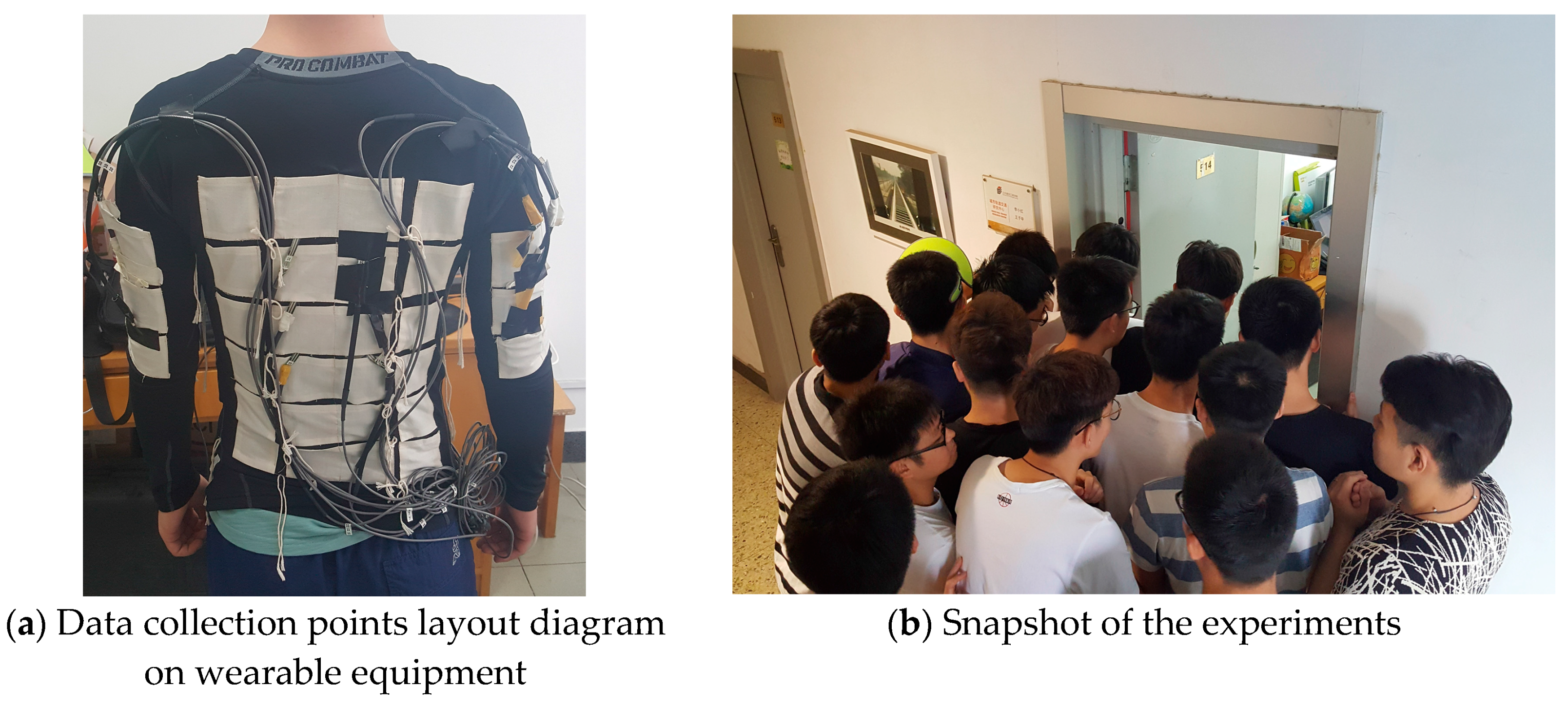
The crowding force in this paper refers to the physical force caused by body contacts. It is an interaction force among two or more pedestrians. When there is an emergency in big and crowded place, pedestrians would scramble with each other to get away from the dangerous area as soon as possible. In this situation, the extrusion may be occurred among a cluster of pedestrians. Therefore, when people touch and press others in a crowded scenario, the crowding force emerges. Pressure sensors are attached onto clothing. There are twelve pressure sensors, produced by Sensor Products Inc. USA, including six pieces on the back and three on each arm to measure the forces. A piece of sensor is a square with a side length of 0.044 m. The sensitivity and frequency are 0.001 KPa and 50 Hz, respectively. And we extract the maximum value at different time points with the same interval when the press among pedestrians happens. The equipment are shown in Figure 4a.

The crowding force test required a participant wearing the cloth with sensors and stand in the middle of a crowd. While entering the bottleneck, the pressure on the participant in different positions was measured. In this manner, the force distribution in the arched area could be described further and most dangerous individual can be identified.

First, we needed to ensure that the experimental scenario was the same as in the simulation. The test area was set at a 1 m-wide door with a 2 m-long channel inside. All the participants waited outside. At the beginning of the test, the testers wear the equipment and were arranged in the congested area in accordance with the same conditions of congestion and squeezing into the door. The crowd started with an initial density of 5.6 ped/m², like the simulation results. The pedestrians were set in a crowded condition; in order to guarantee the safety of participants, they could shout for help when they were about to fall, get trampled, or had difficulty breathing—in which case the experiment would stop immediately. The test procedure can be seen in Figure 4b.

After 45 repeated tests, a large amount of data was obtained. The difference in the time required for whole test between simulation and experiment was within acceptable limits. The simulation result and experimental result were 11.85 s and 12 s, respectively. The error was 1.3%. By extracting the maximum crowding force at each position, which refer to the most dangerous situation could happen at bottleneck, Figure 5a shows the distribution of the crowding force in the arched area. In the arched area, the maximum force is on the right corner of the narrow channel, which can reach 90.7 N. This occurs at 2.4 s for a duration of 0.1 s. The position of the force is the tester’s right arm. The crowding force in this area decreases as the distance from the bottleneck decreases. The crowding force is closely related to the position where the pedestrians stand as the smaller the number of pedestrians on the side, the smaller the magnitude of force exerted on the body as well. Further, the closer the distance from the bottleneck, the more intense the competition among pedestrians is. With more congestion, the mutual extrusion becomes more obvious, so that we get greater crowding forces. In particular, the person closest to the bottleneck not only bears the pushing pressure from the people behind, but also need to handle the effect of the changing width.

The magnitude of the crowding force is different before and after 6.8 s by analyzing the maximum crowding forces. The maximum crowding force is 90.2 N, obtained at 2.4 s. The congestion is slowly disappearing and the maximum crowding force decrease to 5.9 N after the 6.8 s, which is only 6.5% of that before 6.8 s. Figure 5b shows the variation of crowding force with time. We can analyze the increasing of maximum crowding force as it is accompanied with the congestion appearing. It also shows that the crowding phenomenon tends to show up in the early 6.8 s. Over time, the number of people inside the arched area is decreases. Consequently, the interactions among them decrease until the forces reach zero.

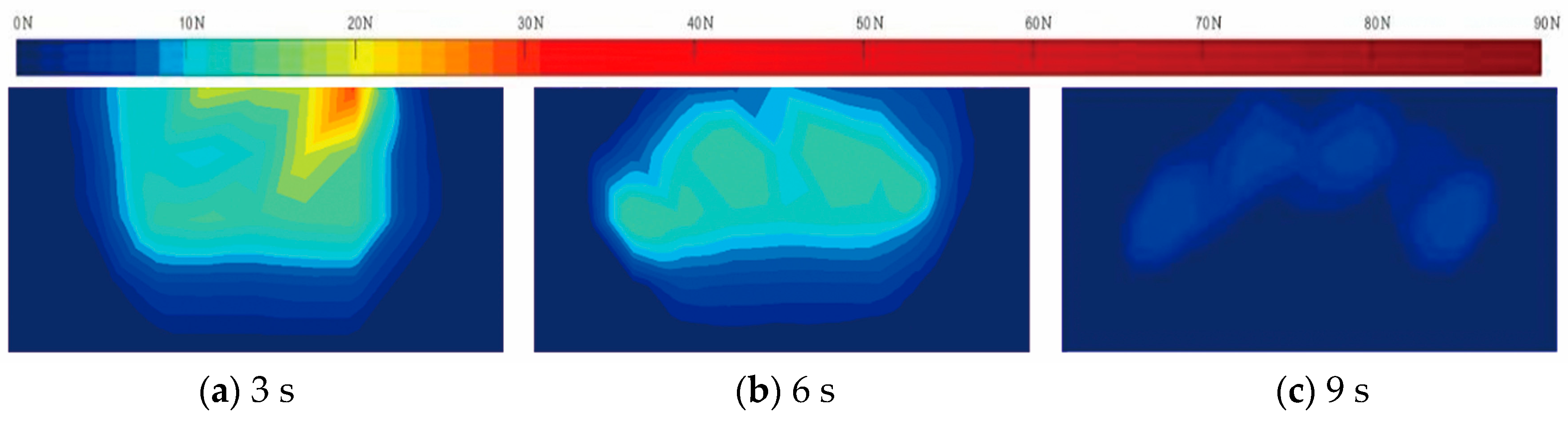
On the other hand, the crowding forces evolutions in different positions are also different. Figure 6 shows the maximum crowding force at each position’s distributions in three phases. At the third second, the person who is closest to the bottleneck is bearing a force of 40 N. At that point, the crowd has reached congestion. At the sixth second, the crowded area begins to collapse slowly. Pedestrians enter the narrow channel more or less and the interactional force is obviously reduced. The crowding force of the group that does not walk into the channel remains at 15 N, which implies that the interaction still exists among pedestrians. At the ninth second, the arched area completely disappeared, and the crowding force decreased to below 5 N. Most of individuals no longer bore pressure, because increasingly more people passed the bottleneck. As we have mentioned above, the empirical maximum contact force a normal adult can bear is 247 N [35]. Generally speaking, what we have got is within the safe range.

In order to discover the behavior of pedestrians’ movement more intensively and how the density and force impact the cluster risk, we extracted the density of the bottleneck simulation and the crowding force of the experiment above in the same scenario to investigate the relationship of this two parameters. We also calculated the crowd densities at different times by analyzing the pedestrian movement recorded by video, comparing with the results we get from macroscopic model to assure the consistency of simulation and experiment. In combination with the pressure test results, the corresponding function between force and density was established. The data were drawn at a 0.5 s interval; the fitting curve is shown in Figure 7. The exponential fitting is used to satisfy the goodness of fit’s condition. R² is found to be 0.98. When the density is less than 5 ped/m², there is no contact and pushing among the pedestrians in the test area, which leads to the force being zero. With the increase of the density, crowding force increases. The two parameters have a positive correlation before the crowding force and density reach 31 N and 8 ped/m². After the force exceeds 31 N, the density increases slowly and within the limits of the maximum density, which is 8.2 ped/m². The main reason for this phenomenon is that the human body does not have substantial elastic deformation, which ensures that the density of the crowd cannot increase indefinitely. When the density reaches a critical value, the space among pedestrians is close to zero, and the congestion becomes increasingly more serious. The crowding force increases no longer leads to an increase in density, but at this point crushing or choking may happen due to the overcrowding. When the slope of this fitting meet 0.01, the fitting is in close proximity to horizontal, which we take as critical point. In this experiment, the critical density value is 8 ped/m² and the critical crowding force is 31 N.

4. Conclusions and Future Research

4.1. Conclusions

In this paper, we studied the macroscopic pedestrian flow model and used the Lax–Wendroff scheme of finite difference method. It was more accurate to analyse the partial differential equations with operator splitting method and Godunov fast sweeping method. The numerical example is carried out simulations of scenarios with obstacle and bottleneck. Then, we introduced the actual crowding force in this research to evaluate the cluster risk of pedestrians’ movement by using pressure sensors. The crowding force test was conducted based on the bottleneck’s simulation results. At last, the relationship between density and crowding force was established by analyzing the data of macroscopic simulation and experiment. The main findings of this study are as follows:

(1)

The maximum force of pedestrians was found to be 90.2 N at 2.4 s and lasting for 0.1 s, on the right side of the narrow channel, which can be deemed the most dangerous position. Under the maximum force, the tester was able to maintain physiological characteristics, but movement was limited. As distance from the bottleneck increased over time, the contact force slowly became zero.

(2)

The pedestrian movement can be divided into two stages (with a 6.8 s dividing line) on the basis of recorded video by comparing the value of maximum crowding force. Before 6.8 s, the crowd congested, which makes the highest density reach 8 ped/m², and the crowding force is also at a higher level. After 6.8 s, the magnitude of the force is significantly reduced. The maximum reduction is 93%, surprisingly, and there are not obvious contact among test people. In the end, the densities of the pedestrian distributions were extracted from the video.

(3)

A fitting exponential function relationship between crowding force and density was proposed. As the crowd cannot compress the deformation infinitely under pressure, the density tends to stabilize at a critical value of 8 ped/m² and no longer increases substantially.

4.2. Future Research

Most researches remains to be conducted on crowding force and density. This study is only a preliminary quantitative analysis. Future researches could involve more in-depth study of the relationship between force and density through experiments, or in combination with a model of contact force such as the social force microscopic model. A cluster risk rating standard can be established for crowding force and crowd density. Using this scientific method, we can judge the hazard level of the pedestrians in high-density conditions, thereby analyzing the safety of pedestrians walking from the perspective of more impeccable evaluation.

References

1. Hankin, B.D.; Wright, R.A. Passenger flow in subways. Oper. Res. Q. 1958, 9, 81–88. [Google Scholar] [CrossRef]
2. Henderson, L.F. The statistics of crowd fluids. Nature 1971, 229, 381–383. [Google Scholar] [CrossRef] [PubMed]
3. Hughes, R.L. The flow of large crowds of pedestrians. Math. Comput. Simul. 2000, 53, 367–370. [Google Scholar] [CrossRef]
4. Hoogendoorn, S.P.; Bovy, P.H.L. Dynamic user-optimal assignment in continuous time and space. Transp. Res. Part B Methodol. 2004, 38, 571–592. [Google Scholar] [CrossRef]
5. Daamen, W.; Hoogendoorn, S.P.; Bovy, P.H.L. First-order pedestrian traffic flow theory. Transp. Res. Rec. 2005, 1934, 43–52. [Google Scholar] [CrossRef]
6. Daamen, W.; Hoogendoorn, S. Calibration of pedestrian simulation model for emergency doors by pedestrian type. Transp. Res. Rec. 2012, 2316, 69–75. [Google Scholar] [CrossRef]
7. Bellomo, N.; Knopoff, D.; Soler, J. On the Difficult Interplay between Life, “COMPLEXITY”, and Mathematical Science. Math. Model. Methods Appl. Sci. 2013, 23, 1861–1913. [Google Scholar] [CrossRef]
8. Elmoussaoui, A.; Argoul, P.; Rhabi, M.E.; Hakim, A. Discrete kinetic theory for 2D modeling of a moving crowd: Application to the evacuation of a non-connected bounded domain. Comput. Math. Appl. 2017. [Google Scholar] [CrossRef]
9. Burini, D.; Chouhad, N. Hilbert method toward a multiscale analysis from kinetic to macroscopic models for active particles. Math. Model. Methods Appl. Sci. 2017, 27, 1327–1353. [Google Scholar] [CrossRef]
10. Bellomo, N.; Dogbé, C. On the modelling crowd dynamics from scaling to hyperbolic macroscopic models. Math. Model. Methods Appl. Sci. 2008, 18, 1317–1345. [Google Scholar] [CrossRef]
11. Dogbé, C. On the numerical solutions of second order macroscopic models of pedestrian flows. Comput. Math. Appl. 2008, 56, 1884–1898. [Google Scholar] [CrossRef]
12. Al-Nasur, S.; Kachroo, P. A microscopic-to-macroscopic crowd dynamic model. In Proceedings of the Intelligent Transportation Systems Conference, Toronto, ON, Canada, 17–20 September 2006; pp. 606–611. [Google Scholar] [CrossRef]
13. Twarogowska, M.; Goatin, P.; Duvigneau, R. Macroscopic modeling and simulations of room evacuation. Appl. Math. Model. 2014, 38, 5781–5795. [Google Scholar] [CrossRef]
14. Jiang, Y.Q.; Zhou, S.G.; Tian, F.B. Macroscopic pedestrian flow model with degrading spatial information. J. Comput. Sci. 2015, 10, 36–44. [Google Scholar] [CrossRef]
15. Jiang, Y.Q.; Guo, R.Y.; Tian, F.B.; Zhou, S.G. Macroscopic modeling of pedestrian flow based on a second-order predictive dynamic model. Appl. Math. Model. 2016, 40, 9806–9820. [Google Scholar] [CrossRef]
16. Hoogendoorn, S.P.; Wageningen-Kessels, F.L.M.V.; Daamen, W.; Duives, D.C. Continuum modelling of pedestrian flows: From microscopic principles to self-organised macroscopic phenomena. Phys. A Stat. Mech. Appl. 2014, 416, 684–694. [Google Scholar] [CrossRef]
17. Duives, D.C.; Daamen, W.; Hoogendoorn, S.P. Continuum modelling of pedestrian flows—Part 2: Sensitivity analysis featuring crowd movement phenomena. Phys. A Stat. Mech. Appl. 2016, 447, 36–48. [Google Scholar] [CrossRef]
18. Cristiani, E.; Peri, D. Handling obstacles in pedestrian simulations: Models and optimization. Appl. Math. Model. 2017, 45, 285–302. [Google Scholar] [CrossRef]
19. Mahato, N.K.; Klar, A.; Tiwari, S. Particle methods for multi-group pedestrian flow. Appl. Math. Model. 2018, 53, 447–461. [Google Scholar] [CrossRef]
20. Shiwakoti, N.; Sarvi, M.; Rose, G.; Burd, M. Animal dynamics based approach for modeling pedestrian crowd egress under panic conditions. Transp. Res. Part B Methodol. 2011, 45, 1433–1449. [Google Scholar] [CrossRef]
21. Soria, S.A.; Josens, R.; Parisi, D.R. Experimental evidence of the “Faster is Slower” effect in the evacuation of ants. Saf. Sci. 2012, 50, 1584–1588. [Google Scholar] [CrossRef]
22. Helbing, D.; Isobe, M.; Nagatani, T.; Takimoto, K. Lattice gas simulation of experimentally studied evacuation dynamics. Phys. Rev. E 2003, 67, 067101. [Google Scholar] [CrossRef] [PubMed]
23. Yamamoto, S.; Hieida, Y.; Tadaki, S.I. Effects of Bottlenecks on Vehicle Traffic. J. Phys. Soc. Jpn. 2006, 75, 114601. [Google Scholar] [CrossRef]
24. Gorrini, A.; Bandini, S.; Sarvi, M. Group Dynamics in Pedestrian Crowds Estimating Proxemic Behavior. Transp. Res. Rec. 2014, 2421, 51–56. [Google Scholar] [CrossRef]
25. DiNenno, P.J. SFPE Handbook of Fire Protection Engineering; SFPE: Quincy, MA, USA, 2008. [Google Scholar]
26. Predtechenskii, V.; Milinski, A.I. Planning for Foot Traffic Flow in Buildings; National Bureau of Standards, US Department of Commerce, and the National Science Foundation: Washington, DC, USA, 1978.
27. Daamen, W.; Hoogendoorn, S.P. Emergency door capacity: Influence of door width, population composition and stress level. Fire Technol. 2012, 48, 55–71. [Google Scholar] [CrossRef]
28. Kretz, T.; Grünebohm, A.; Schreckenberg, M. Experimental study of pedestrian flow through a bottleneck. J. Stat. Mech. Theory Exp. 2006, 10. [Google Scholar] [CrossRef]
29. Kretz, T.; Hengst, S.; Vortisch, P. Pedestrian flow at bottlenecks-validation and calibration of vissim’s social force model of pedestrian traffic and its empirical foundations. In Proceedings of the 2008 International Symposium of Transport Simulation, Gold Coast, Australia, 6–8 August 2008. [Google Scholar] [CrossRef]
30. Cirillo, E.N.M.; Colangeli, M.; Muntean, A. Trapping in bottlenecks: Interplay between microscopic dynamics and large scale effects. Phys. A Stat. Mech. Appl. 2017, 488, 30–38. [Google Scholar] [CrossRef]
31. Mcphail, C. The Myth of the Madding Crowd; Walter de Gruyter: New York, NY, USA, 1991. [Google Scholar]
32. Canetti, E. Crowds and Power; Phoenix Press: London, UK, 2000. [Google Scholar]
33. Lee, R.S.C.; Hughes, R.L. Exploring trampling and crushing in a crowd. J. Transp. Eng. 2005, 131, 575–582. [Google Scholar] [CrossRef]
34. Henein, C.M.; White, T. Macroscopic effects of microscopic forces between agents in crowd models. Phys. A Stat. Mech. Appl. 2007, 373, 694–712. [Google Scholar] [CrossRef]
35. Smith, R.A.; Lim, L.B. Experiments to investigate the level of ‘comfortable’ loads for people against crush barriers. Saf. Sci. 1995, 18, 329–335. [Google Scholar] [CrossRef]
36. Helbing, D.; Johansson, A.; Al-Abideen, H.Z. Dynamics of crowd disasters: An empirical study. Phys. Rev. E 2007, 75, 046109. [Google Scholar] [CrossRef] [PubMed]
37. Ma, J.; Song, W.G.; Lo, S.M.; Fang, Z.M. New insights into turbulent pedestrian movement pattern in crowd-quakes. J. Stat. Mech. Theory Exp. 2013, 2013, 02028. [Google Scholar] [CrossRef]
38. Yin, H.; Li, D.; Zheng, X. An energy based method to measure the crowd safety. Transp. Res. Procedia 2014, 2, 691–696. [Google Scholar] [CrossRef]
39. Harlow, F.H.; Fromm, J.E. Computer experiments in fluid dynamics. Sci. Am. 1965, 212, 104–110. [Google Scholar] [CrossRef]
40. Harten, A.; Lax, P.D.; Leer, B.V. On upstream differencing and Godunov-Type schemes for hyperbolic conservation laws. SIAM Rev. 1983, 25, 35–61. [Google Scholar] [CrossRef]
41. Huang, L.; Wong, S.C.; Zhang, M.; Shu, C.W.; Lam, W.H. Revisiting Hughes’ dynamic continuum model for pedestrian flow and the development of an efficient solution algorithm. Transp. Res. Part B Methodol. 2009, 43, 127–141. [Google Scholar] [CrossRef]
42. Zuriguel, I.; Janda, A.; Garcimartín, A.; Lozano, C.; Arévalo, R.; Maza, D. Silo clogging reduction by the presence of an obstacle. Phys. Rev. Lett. 2011, 107, 278001. [Google Scholar] [CrossRef] [PubMed]
Figure 1. Sketch of a simple model.
Sustainability 10 00385 g001
Figure 2. Density distribution evolution: (a) model size; (b) density evolution.
Sustainability 10 00385 g002
Figure 3. Model size and simulation results.
Sustainability 10 00385 g003aSustainability 10 00385 g003b
Figure 4. Experimental situations.
Sustainability 10 00385 g004
Figure 5. Crowding force distribution evolution.
Sustainability 10 00385 g005
Figure 6. Crowding force distribution at different times (unit: N).
Sustainability 10 00385 g006
Figure 7. Fitting curve of the crowding force-density relationship.
Sustainability 10 00385 g007