Optimized Planning of Different Crops in a Field Using Optimal Control in Portugal

Abstract

Climate change is a proven fact. In the report of 2007 from IPCC, one can read that global warming is an issue to be dealt with urgently. In many parts of the world, the estimated rise of temperature (in a very near future) is significant. One of the most affected regions is the Iberian Peninsula, where the increasing need for water will very soon be a problem. Therefore, it is necessary that decision makers are able to decide on all issues related to water management. In this paper, we show a couple of mathematical models that can aid the decision making in the management of an agricultural field at a given location. Having a field, in which different crops can be produced, the solution of the first model indicates the area that should be used for each crop so that the profit is as large as possible, while the water spent is the smallest possible guaranteeing the water requirements of each crop. Using known data for these crops in Portugal, including costs of labour, machines, energy and water, as well as the estimated value of the products obtained, the first mathematical model developed, via optimal control theory, obtains the best management solution. It allows creating different scenarios, thus it can be a valuable tool to help the farmer/decision maker decide the crop and its area to be cultivated. A second mathematical model was developed. It improves the first one, in the sense that it allows considering that water from the rainfall can be collected in a reservoir with a given capacity. The contribution of the collected water from the rainfall in the profit obtained for some different scenarios is also shown.

1. Introduction

Climate change is a proven fact. In the report of 2007 from IPCC [1], one can read that global warming is an issue to be dealt with urgently. Temperature will raise, and longer and more frequent draught periods will occur. One of the most affected regions will be the Iberian Peninsula. In the south of Iberia, extreme draught periods are already very frequent. Our study considered Portugal, but it could easily be adapted to another part of the world. In this scenario, it is necessary that the decision makers are able to decide on all issues related to water management.

Irrigation of crop fields spends the most water resources in Portugal annually. Thus, it becomes crucial that a proper irrigation plan can maximize the profits of a crop field, while spending the least water resources possible, with the highest efficiency [2]. In this paper, the authors contribute to achieving such an objective.

The first mathematical model presented in this paper was implemented in MatLab, based on optimal control theory. It allows considering different crops in the same field, and it can plan the percentage of the area to be allocated for each crop, in such a way that the profit is maximum, while minimizing the water spent, and assuring the water requirements of each crop. This could be a valuable tool when a farmer intends to cultivate a field from scratch with different crops. It is not intended that the farmer changes the area of each crop when it is already cultivated. On the other hand, by changing very few parameters, it is possible rethink the crops to have in that field. This model has as inputs the weather variables, the location of the field, the type of soil, the value of the crops, the costs of the crops, and the cost of water.

A second model improves the first one, giving the information on the profit obtained when water from rainfall is collected in a reservoir of a given capacity, allowing to save water while keeping the crop safe.

The models can be improved taking into account a prediction of the weather variables and economic variables using for example time series. It can be easily adapted to a different location or crops depending on the available data.

Optimal control theory emerged as a field of research in the 1950s in response to problems concerning the aerospace exploitation [3] of the solar system. Nowadays, optimal control is a recognized tool, known for its efficacy, which is applied to different areas, such as robotics [4], biological systems [5], health problems [6], economy problems [7], oil extraction problems [8], and agriculture problems [9], among many others. The goal of optimal control theory is to find a control law for a given system such that a certain optimality criterion is achieved.

In optimal control problems (OCP), it is possible to define decision variables subject to restrictions in the form of differential equations, where these decisions variables are not necessarily smooth (non-differentiable functions). In an OPC, it is also possible to use different tools to solve the problem, to characterize it, to study the sensitivity of its variables, to study the stability of the problem and to apply predictive control to replan the problem [9,10,11]. The nature of the problems addressed in this paper is fit for optimal control theory.

The literature includes publications that have similar objectives, although they use different formulations and techniques to solve them. Osama, Elkholy and Kansoh in [12] developed a linear programming model for optimal land allocations for different crops in Egypt. Different constraints were incorporated in the model, including the water availability, the land availability in different seasons of the year, self-sufficiency ratios and the areas for each crop under the existing cropping pattern. The authors imposed that the total water requirement for the different crops, should be less or equal than the total water available at the field during the year. However, the irrigation water optimization was not considered.

Kuo, Merkleyb, and Liu [13] developed a decision support model for an irrigation project plan (in Utah), using a genetic algorithm (GA) optimization method. This model allows optimizing the profits, simulating the water demand and crop yields, and estimating the related crop area percentages with specified water supply and planted area constraints.

Dutta [14] developed a multi-objective fuzzy stochastic model for determination of optimum cropping patterns for the next crop season guaranteeing the water balance. The objective of the model is to study the effect of various cropping patterns on crop production subject to total water supply in a small farm. The model is implemented using fuzzy stochastic simulation, based on a genetic algorithm, without deriving the deterministic equivalents. However, the solution using a direct method is faster and more accurate than using genetic algorithms (models by Kuo [13] and Dutta [14]). In addition, genetic algorithms need an initial solution to start the process which might not be easy to find (see [15]).

In our study, direct methods in optimal control (such as Interior Point OPTimizer (IPOPT), Sequential quadratic programming (SQP), Active Set, etc), which guarantee that a feasible solution is obtained, were used. In similar mathematical models (to the ones presented in this article), it is proven that the obtained solution is a local extrema [16]. The first model presented in this article is able to plan the percentage of area for each crop in such a way that the profit is maximum, while minimizing the water spent and assuring the water requirements of each crop. The optimal control theory allows defining an objective function that is the sum of the profits obtained for each crop, taking into account the value of the crop, the costs of production, the costs of water, and the type of weather conditions.The dynamic equation considered guarantees the water balance (taking into account rainfall, irrigation, humidity in the soil, evapotranspiration and losses due to infiltration), the constraints considered guarantee that the crops have their needs of water fulfilled. Therefore, this model is better than others based on GA, and assures that water balance is never broken. On the other hand, optimal control is able to guarantee a smoother solution, not present in “on–off” type irrigation systems, since the weather and an economic forecast are used.

The possibility for the farmer to build a reservoir (also considered in [17]) of a given capacity to collect rainwater was considered, and it was the basis for the second mathematical model proposed in this paper. Since climate change is showing us that water availability is going to drop, planning a proper reservoir to collect rainfall is crucial to preserve the crops and increase profit. It is possible to use the second model to solve the problem where there is no reservoir. However, the number of variables involved double, and the CPU time to solve it is greatly increased.

This paper is divided into five sections. The Introduction is presented in the Section 1. In Section 2, two models for optimized management of a field with several crops are presented. Data for the numerical model are introduced in Section 3. Results for each model are shown and discussed in Section 4. Finally, conclusions are presented in Section 5. Two appendixes are also included at the end of the paper.

2. Mathematical Models Considered

In this section, two mathematical models in the same framework are presented. The first model maximizes the profit of a field with several crops while minimizing the water consumption in irrigation and keeping the crops safe. It also gives the farmer information on which percentage of the area should be allocated to each crop. A second model considers the possibility that the farmer builds a reservoir of a given capacity to collect rainwater.

2.1. Management of a Field with Several Crops Using the Profit as Objective Function

In optimal control problems, there are two types of variables: the state and the control variables. The state variables are defined through differential equations and the control variables are the decision variables to minimize (or maximize) an objective function.

The state variables are the following: $x_i$ is the amount of water in the soil (m${}^3$ per m${}^2$) for the sub-field i. The control variables are defined as: $u_i$ is the water (m${}^3$/month per m${}^2$) introduced in sub-field i via its irrigation system and $A_i$ is the percentage of the area of each sub-field i. It is assumed that in each sub-field exists only one crop.

The objective function is the sum of the revenue of each crop:

$$\sum _{i=1}^N\left({C_C}_i-{C_P}_i-10000P_W{\int }_0^T{u}_i\left(t\right)dt\right)A_i$$

(1)

where T is the number of months considered in the model, N is the number of sub-fields with a certain crop, $C_C$ is the value of that crop (euro/hectare), $P_W$ is the price of water per m${}^3$, 10,000 $u_i$ is the irrigation per hectare, and $C_P$ is the cost of production (euro/hectare) of the crop (including labour, machines, and energy, among others) [18,19,20] defined as:

$${\displaystyle {C_P}_i\left(A_i\right)=\left\{\begin{array}{cc}{K}_i(1-{A_i}^2),\hfill & A_i\le 0.25\hfill \\ K_i(0.9375+0.25{(A_i-0.25)}^2),\hfill & 1\ge A_i>0.25\hfill \end{array}\right.}$$

(2)

where $K_i$ is a constant that ensures that the average cost of crop i ($AV{C}_i$) has a certain value per hectare, which can be consulted in literature (${\int }_0^1{C_P}_i\left(A_i\right)d{A}_i=AV{C}_i$). This function assumes the costs are greater for smaller areas, then decreases until a certain area value, and finally increases again, as shown in Figure 1. The function is a mathematical attempt to describe this behavior for the cost. The constants present in the above formula are such that the costs of the crop as function of its area are a continuous function. Note that data on average cost values as function of the area are not available.

We note that this function can be easily replaced by the real cost values per area for each crop in the Matlab programme that was developed.

The variation of the water in the soil is given by the water balance equation [21]. Water enters from irrigation systems (u) and precipitation (g in m${}^3$/month per m${}^2$), water exits via evapotranspiration (h in m${}^3$/month per m${}^2$) and percolation ($\beta x$ in in m${}^3$/month per m${}^2$). $\beta$ (in percentage/month) is a parameter that depends on the type of soil. The model of percolation has been defined in order that the humidity of the soil decreases exponentially, as in Horton’s equation [22].

Therefore, for each sub-field i, the water balance equation is given by:

$${\dot{x}}_i\left(t\right)=u_i\left(t\right)+g\left(t\right)-h_i\left(t\right)-\beta x_i\left(t\right),\forall i=1,\dots ,N.$$

(3)

We note that each sub-field has only one crop. To ensure that the crop does not die because of lack of water, the water in the soil has to be greater or equal to the hydric needs of each crop $x_{{min}_i}$.

$$x_i\left(t\right)\ge x_{{min}_i}\forall i=1,\dots ,N.$$

(4)

$A_i$ is the percentage of the total area that is devoted to crop i. It is assumed that at least two crops exist, meaning that $A_i$ is never 0. In our programme. we considered that

$$0.1\le A_i\le 0.9,\forall i=1,\dots ,N$$

(5)

Note that the sum of all $A_i$ is equal to 1.

$$\sum _i{A}_i=1.$$

(6)

The control variable is bounded by,

$$u_i\left(t\right)\in [0,M_i],\forall i=1,\dots ,N$$

(7)

where $M_i$ is the maximum value of irrigation. In theory, it could be infinite, but the model demands it to be finite. It was considered to be a very large number. The initial values of the water in the soil for each culture $x_{0_i}$ are given as

$$x_i\left(0\right)=x_{0_i},\forall i=1,\dots ,N$$

(8)

2.2. Using Reservoir for Rainwater Collection

The model presented in this section improves the last one. This model contemplates the possibility that the farmer intends to build a reservoir to collect water from rainfall.

In this new model, the state variables are the following: $x_i$ is the water in the soil of sub-field i and y is the total of amount of water stored in reservoir (in m${}^3$ per m${}^2$). The control variables are defined as: $u_i$ is the water flow introduced in sub-field i via its irrigation system (in this case the water comes from the tank), $A_i$ is the percentage of the area of each sub-field i and v is the water flow coming from the water supply network ( in m${}^3$/month per m${}^2$).

The objective function is the sum of the revenue of each crop:

$$\left(\sum _{i=1}^N({C_C}_i-{C_P}_i)A_i-10000P_W{\int }_0^{T}v\left(t\right)dt\right),$$

(9)

where ${\int }_0^{T}v\left(t\right)dt$ is the total amount of water from the water supply network to fill the tank if necessary. The equation that stands for the water balance in the field does not change.

The variation of water in reservoir is equal to the water flow coming from the water supply network (v), plus the water that is collected from the precipitation $Pg\left(t\right)$ ( in m${}^3$/month per m${}^2$), minus the water used in the irrigation systems for each sub-field ${\sum }_{i=1}^N{A}_i{u}_i\left(t\right)$. The variation of water in reservoir is written as:

$$\dot{y}\left(t\right)=v\left(t\right)+Pg\left(t\right)-\sum _{i=1}^N{A}_i{u}_i\left(t\right),$$

(10)

where P is the percentage of water from rainfall that is collected, and g is the precipitation (in m${}^3$/month per m${}^2$) at the time t.

The maximum amount of water in the tank is $y_{max}$,

$$y\left(t\right)\in [0,y_{max}],\forall t\in [0,T],$$

(11)

where $y_{max}$ is the maximum amount of water in the reservoir.

The value of the flux of water taken from the water supply network is limited,

$$v\left(t\right)\in [0,V_{max}]$$

(12)

where $V_{max}$ is necessary to impose in order to obtain a limited interval for $v\left(t\right)$.

The initial amount of water in the tank is,

$$y\left(0\right)=y_0,$$

(13)

where $y_0$ is a given value. The detailed optimal control formulations of the problems described in Section 2.1 and Section 2.2 are in Appendices Appendix A and Appendix B.

3. Data for the Numerical Model

The models presented in the previous section allow considering many crops. Since we chose Portugal as the study site, we had to use crops that are widely cultivated there, and for which we had enough data. We considered only two crops so that the results are easier to present. The crops considered in our study were olive trees and vines. Using known data from these cultures in Portugal, including cost of labour, machines, energy and water, as well as the estimated value of the products obtained per hectare, it was possible to determine the cost function of each crop per hectare. The cost function used, as explained in previous sections, takes into account these data.

In the rural region of the Lisbon district, the values of olives and grapes are in the interval of [750, 1760] euro/ hectare and [2700, 3300] euro /hectare, respectively. The price of water is 0.07 euro/m${}^3$, the cost of labour, machines, energy and services are on average 700 euro/hectare for olive trees and 2780/hectare for vines [18,19,20].

We also considered the rainfall to be the average of the rainfall in the last 10 years for each month of the year, as shown in

Table 1. Average of the rainfall in the last 10 years for each month of the year in (10${}^{-3}$ m${}^3$/month) per m${}^2$.

J	F	M	A	M	J	J	A	S	O	N	D
111.4	94.7	80.2	57.1	29.6	18.8	1.3	7.0	30.6	127	122	119.3

[23].

To create the possibility of different weather scenarios, the above table is multiplied by a precipitation factor:

$$rainfall\left(t_i\right)=\mathit{precipitationfactor}\times \mathit{rainmonthlyaverage}\left(t_i\right),$$

(14)

where the precipitation factor allowed us to consider a typical year if this factor is 1, a drought year if it is less that 1 and a rainy year if it is above 1 [24].

The Pennman–Monteith methodology [25] was used to calculate evapotranspiration of the cultures along the year, from the following equation

$$ET\left(t_i\right)=K_{c}E{T}_0\left(t_i\right),$$

(15)

where $K_c$ is the culture coefficient for the evapotranspiration and $E{T}_0$ is the tabulated reference value of evapotranspiration from [26] for the Lisbon region. The evapotranspiration of the cultures in Lisbon is given in

Table 2. The evapotranspiration of the cultures in Lisbon is given by the following table in (${10}^{-3}$ m${}^3$/month) per m${}^2$.

J	F	M	A	M	J	J	A	S	O	N	D
19.8	28.0	55.3	89.1	116.3	137.8	155.9	136.9	85	53.6	22.3	16.5

.

The following data were also considered to perform simulations in Section 4:

$$\begin{array}{c}T=11\left(\mathrm{month}\right)\hfill \\ x_0=x_{min}\left({\mathrm{m}}^3\mathrm{per}{\mathrm{m}}^2\right)\hfill \\ \beta =15\%\mathrm{per}\mathrm{month}\hfill \\ M_i=0.2({\mathrm{m}}^3/\mathrm{month}\mathrm{per}{\mathrm{m}}^2)\hfill \\ y_{max}=\left[111110000111\right]\left({\mathrm{m}}^3\mathrm{per}{\mathrm{m}}^2\right)\hfill \\ V_{max}=1({\mathrm{m}}^3/\mathrm{month}\mathrm{per}{\mathrm{m}}^2)\hfill \\ y_0=0\left({\mathrm{m}}^3\mathrm{per}{\mathrm{m}}^2\right)\hfill \end{array}$$

4. Results

In this section, the results from the models described in Section 2.1 and Section 2.2 are presented for a set of different scenarios. Here, it is possible to see how changes in weather conditions, economic conditions, etc. can affect the value of the profit obtained.

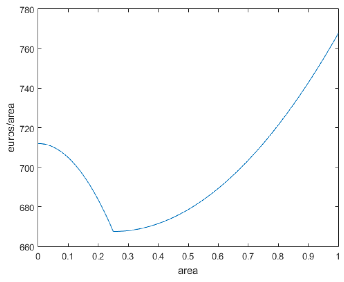
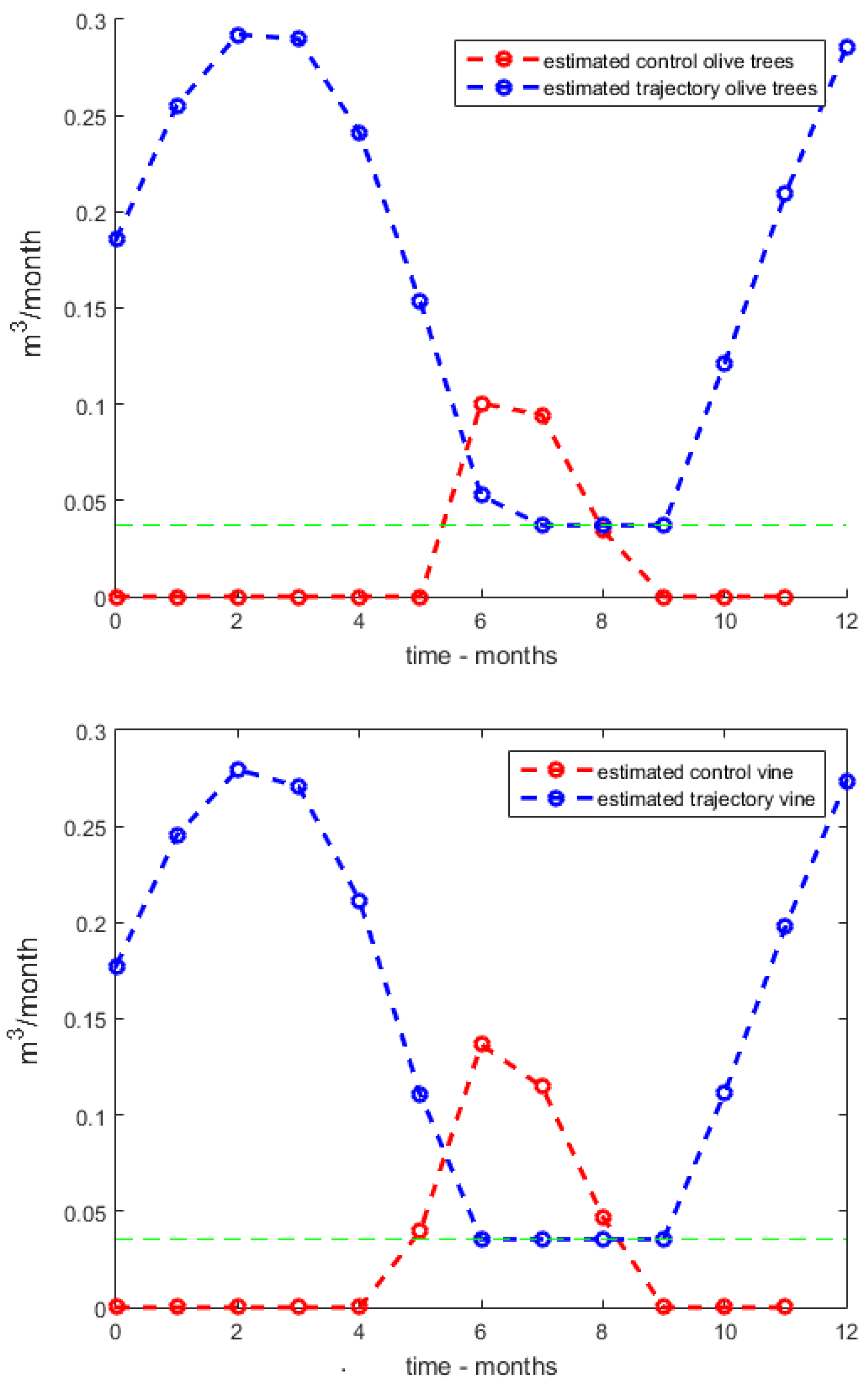
4.1. Results for the Model Presented in Section 2.1

In this subsection, we start by presenting the results of the model in Section 2.1, for medium scenario, called base scenario. We considered the following parameters for the base scenario: value of olives is $V_1=1100$ euro/hectare, value of grapes is $V_2=3100$ euro/hectare, price of the water os $CW=0.07$ euros/m${}^3$, the cost of labour, machines, energy and services (production costs) are on average $Ap{c}_1=700$ euro/hectare for olive trees and $Ap{c}_2=2780$ euro/hectare for grapes, defined in a cost function dependent on the area, as explained in Section 2.1. Using the base scenario, we obtained the results in

Table 3. Results for base scenario.

Description	Notation	Result
profit	Prf	230.25 euro/hectare
area of olive trees	$A_1$	$64.6\%$
water spent in olive trees	$W_1$	1481 m${}^3$/hectare
water spent in vines	$W_2$	1196 m${}^3$/hectare
production costs for olive trees	$C{P}_1$	695.4 euro/hectare
production costs for vines	$C{P}_2$	2658 euro/hectare.

.

We also created weather scenarios with the precipitation factor (F). It is considered an average precipitation when precipitation factor (F) is 1, while, if it is above 1, it means a rainy year, and, if is is below 1, it means a drought year.

We created many possible scenarios (S), which gave completely different results, as it can be read in

Table 4. List of the scenarios considered and results obtained.

S	F	${\mathit{V}}_1$	${\mathit{V}}_2$	CW	${\mathit{Apc}}_1$	${\mathit{Apc}}_2$	Prf	${\mathit{A}}_1$	${\mathit{W}}_1$	${\mathit{W}}_2$	${\mathit{Cp}}_1$	${\mathit{Cp}}_2$
B	1	1100	3100	$0.07$	700	2780	230	$64\%$	1481	1196	695	2658
1	1	1750	3333	$0.07$	700	2780	782	$90\%$	2063	338	743	2799
2	1	750	2666	$0.07$	700	2780	−147	$72\%$	1650	947	706	2651
3	1	750	3333	$0.07$	700	2780	189	$33\%$	756	2265	669	2778
4	1	1750	2666	$0.07$	700	2780	725	$90\%$	2063	338	743	2799
5	1	1100	3100	$0.04$	700	2780	311	$62\%$	1421	1285	692	2662
6	1	1100	3100	$0.14$	700	2780	45	$71\%$	1627	981	705	2652
7	1	1100	3100	$0.07$	770	3400	44	$90\%$	2063	338	828	3420
8	1.2	1100	3100	$0.07$	700	2780	265	$64\%$	1163	1025	695	2658
9	0.25	1100	3100	$0.14$	700	2780	−276	$74\%$	3355	1512	709	2650

. Note in Scenarios 1–4 the only data that change are the values of product 1 (olives, obtained from olive trees) and product 2 (grapes, obtained from vines). In Scenarios 5 and 6, everything is equal to the base scenario, except the price of water ($CW=0.07$ euros/m${}^3$ versus $CW=0.14$ euros/m${}^3$). In Scenario 7, the only difference to the base scenario is that the production costs of olives grew by 10% and the production costs of vine grew by 20%. In Scenarios 8 and 9, the only differences with the base scenario are the value of the precipitation factor (F = 1.2 versus F = 0.25) and the price of water (only in Scenario 9, $CW=0.14$ euros/m${}^3$). In Scenario 8, we have a rainy year, and, in Scenario 9, we have a very severe draught year. In Scenario 9, the price of water increases because the country is facing a severe draught.

In Figure 2, we may see the results for water in the soil (blue line is the trajectory) and the irrigation needed (red line is the control) per m${}^2$ in each month, for each crop for the base scenario. As expected, irrigation starts in May/June and ends in September of the year in study. This is a normal result since we are considering an average year in Portugal. The months where rain becomes scarce are May, June, July and August.

In Scenarios 1–4, we see that the profit (Prf in Table 4) is highly dependent on the value of the products. In Scenarios 5 and 6, the influence of price of water was studied. Once again, we verify that, if the price of water increases (which is expected in the near future), the profit results drop significantly. In Scenario 7, we studied the influence of growing costs of production. In such a case, the profit can become loss very easily. To obtain a better model, provided enough data are available, a time series study could be used to better estimate the costs of production. In Scenario 8 (see Table 4), the rainfall is 20% above normal year rainfall, so the irrigation will be less used. Note the area below the red line and above the time axis is smaller in Figure 3 than the one in Figure 2. This means that less water is spent in Scenario 8 than is the base scenario. Once again, this is not a surprise since, if it rains more, irrigation needs are smaller.

In Scenario 9 (see Table 4), the rainfall is 75 % below normal year rainfall, so irrigation will increase greatly, and, consequently, the price of water will increase. This is a drought year. Note the area below the red line and above the time axis is much larger in Figure 4 than the one in Figure 2. In addition, irrigation starts earlier and ends later in the year. Studying the pattern of the precipitation and its tendency along the years to come is very important.

In Table 4, one may see that, by changing the scenario, the expected profit changes greatly, as does the area dedicated for each crop. As expected, the value of the crops that the farmer obtains for each crop is essential for a good profit. The most important conclusion is that, by changing the price of water (that will increase for sure in a near future) or the precipitation factor (F) for a smaller value (draughts are expected to be more severe and occur more often in Portugal), the profit transforms into loss very easily. This tells us that any means of increasing the efficiency of water used in irrigation, or by collecting the rainfall into a reservoir is essential. In addition, by running our programme, the decision maker may decide to consider other types of crops that may not need so much water. All he has to do is to change a few parameters that are associated to the crops and rerun the programme.

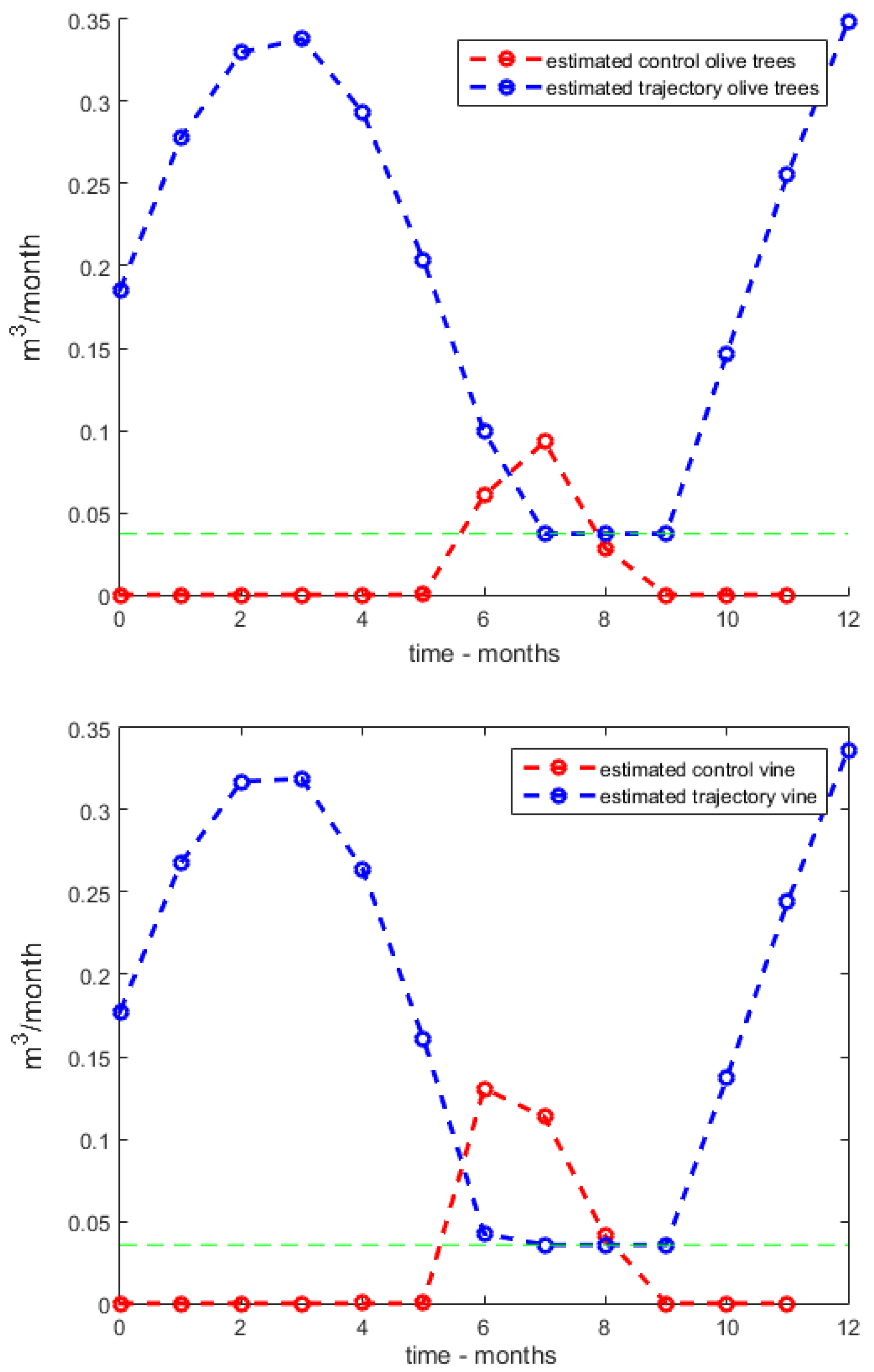
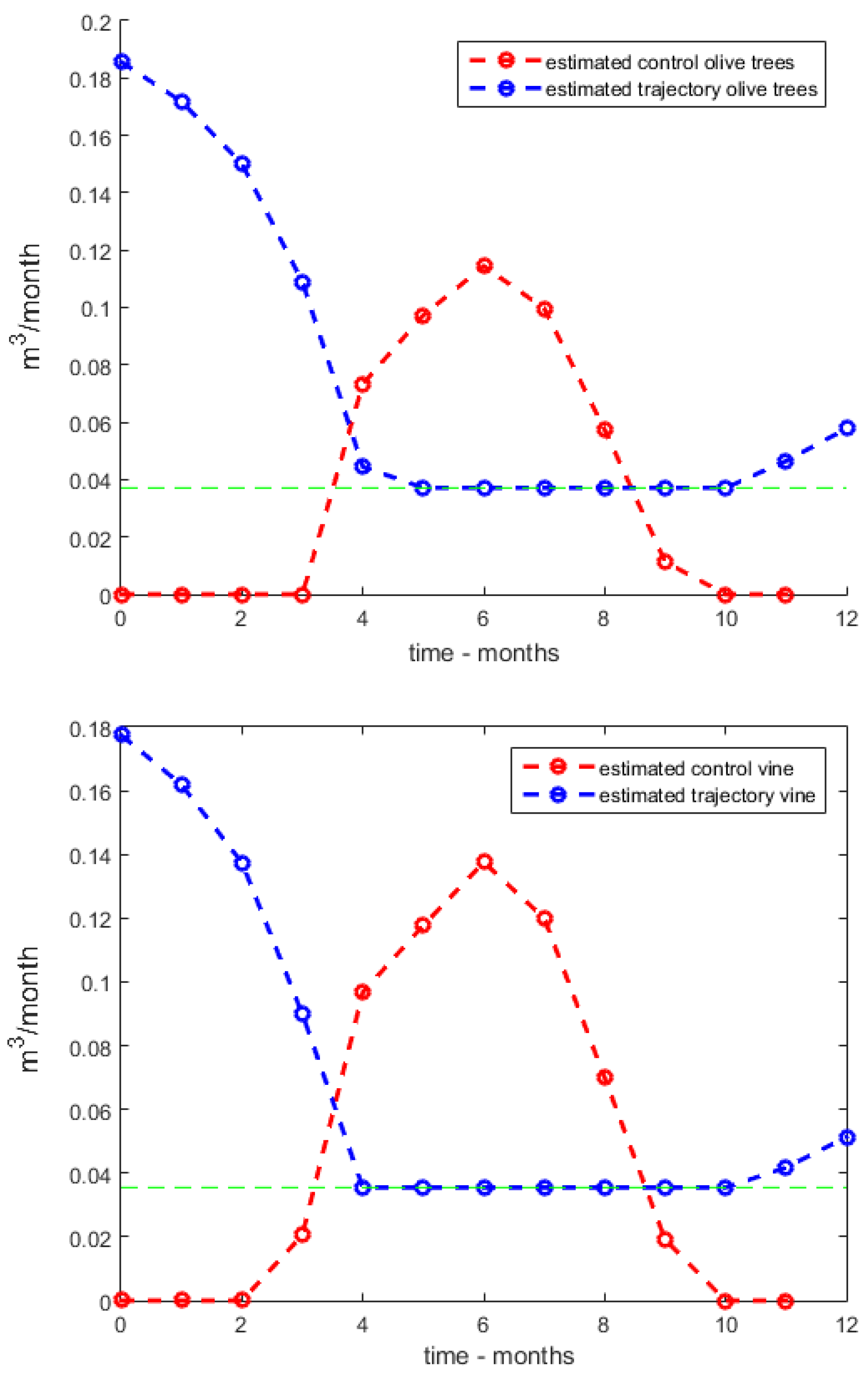
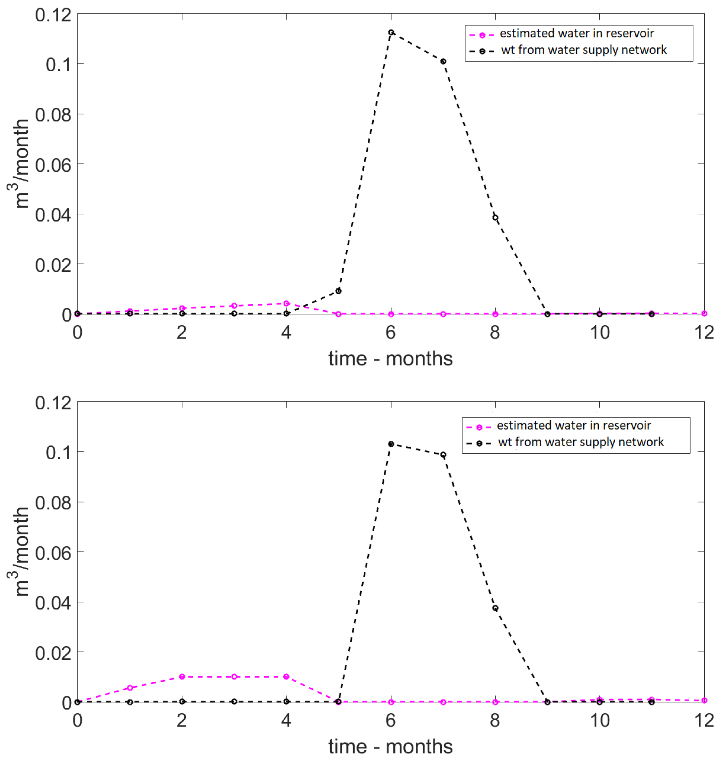
4.2. Results for the Model Presented in Section 2.2—With a Reservoir to Collect Rainfall

To test the second mathematical model, the base scenario used is the same as for the first mathematical model. As expected, the numerical results are the same (see Table 3 and

Table 5. Results for the base scenario using the second mathematical model.

Description	Notation	Result
profit	Prf	230.25 euro/hectare
area of olive trees	$A_1$	$64.6\%$
water spent in olive trees	$W_1$	1481 m${}^3$/hectare
water spent in vines	$W_2$	1196 m${}^3$/hectare
percentage of water collected	P	$0\%$
water used from the tap	$W_T$	2677 m${}^3$/hectare
water cost	$W_c$	1874 euro/hectare
production costs for olive trees	$C{P}_1$	695.4 euro/hectare
production costs for vines	$C{P}_2$	2658 euro/hectare

).

In the case that water from the rainfall is collected, it is important to know how the profit changes. Two scenarios were simulated. In the first one, $1\%$ of water from rainfall is collected and, in the second one, $5\%$ of water from rainfall is collected. In the first case, the profit increased to 235 euro/hectare and in the second one the profit increased to 250 euro/hectare. The total water used decreased to 0.2613 m${}^3$ per m${}^2$ of area and 0.2393 m${}^3$ per m${}^2$ of area, respectively, in the first and second scenarios. In Figure 5, it is possible to see the variation of the water in the reservoir and the amount of water used from the water supply network.

Another important issue is to study how a drought year affects the farmer’s results if he builds a reservoir to collect rainwater with a certain capacity. To do so, we considered the factor precipitation $F=0.25$. Different situations are considered. The percentage of water that is collected in the reservoir is $P=1\%$ or $P=5\%$ of the rainwater, and the price of water is $CW=0.07$ or $CW=0.14$ euros. Results can be seen in

Table 6. Results considering different prices of water ($CW$) and percentage of rainfall collected in the reservoir (P).

Desc	$\mathit{P}=0.01$	$\mathit{P}=0.05$	$\mathit{P}=0.05$
	$\mathit{CW}=0.07$	$\mathit{CW}=0.07$	$\mathit{CW}=0.14$
Prf	$69.85$	$75.08$	$-263.26$	euro/hectare
$A_1$	$65.66\%$	$65.66\%$	$73.47\%$
$W_1$	2978	2979	3334	m${}^3$/hectare
$W_2$	1998	1999	1544	m${}^3$/hectare
$W_T$	4950	4882	4782	m${}^3$/hectare
$W_c$	347	342	669	euro/hectare
$C{P}_1$	$696.9$	$696.9$	709	euro/hectare
$C{P}_2$	2658	2659	2651	euro/hectare

.

Note that, in the near future, severe draughts will occur with a higher frequency. Chances are that governments will no longer be able to subsidise the price of water. This means we could face a situation such as the one in the fourth column of Table 6.

5. Conclusions

Climate change and global warming are facts and are here to stay. In many parts of the world, the estimated rise of temperature for a very near future is significant, and water shortages will happen. One of the most affected regions is the Iberian Peninsula. In Portugal, most water is spent in agriculture, thus a proper irrigation plan is crucial. It is necessary that the crops chosen are the best fit for the farm field, the least amount of water (keeping the crops safe) is spent, the economic results are good and the efficiency in the use of water is as high as possible.

A first mathematical model, based on optimal control theory was implemented in Matlab. Its inputs were the weather variables, the location (the results presented consider the area of Lisbon in Portugal), the type of soil, the value of the crops, the costs of the crops, and the cost of water. The outputs were profit, the percentage of the area to be allocated to each crop, and an irrigation plan for the farm that guarantees the crops are safe.

A second model (also implemented in MatLab and based on optimal control theory) improved the first one, by giving the farmer the possibility of building a reservoir of a given capacity to collect rainwater, and therefore improving the profits and spending less water. The outputs were the profit, the percentage of the area to be allocated to each crop, the amount of water in the tank, and an irrigation plan for the farm that guarantees the crops are safe.

We believe the models developed can help to make the best management decisions when designing (partially designing) a crop field. The developed Matlab application can be easily adapted to a different location or crops.

The presented mathematical models can be improved, taking into account a prediction of the weather variables and economic variables, using for example time series.

References

1. IPCC. Intergovernmental Panel on Climate Change Fourth Assessement Report on Climate Change 2007: Symthetis Report—Summary for Policy Makers; IPCC: Geneva, Switzerland, 2007; ISBN 92-9169-122-4. [Google Scholar]
2. Haie, N.; Pereira, R.M.S.; Machado, G.; Keller, A.A. Analysis of Effective Efficiency in decision making for irrigation interventions. Water Resour. 2012, 6, 700–707. [Google Scholar] [CrossRef]
3. Longuski, J.M.; Guzmán, J.J.; Prussing, J.E. Optimal Control With Aerospace Applications; Springer: Berlin, Germany, 2014; ISBN 978-1-4614-8945-0. [Google Scholar]
4. De Jager, B.; Van Keulen, T.; Kessels, J. Optimal Control of Hybrid Vehicles; Springer: London, UK, 2013; ISBN 978-1-4471-5076-3. [Google Scholar]
5. Lenhart, S.; Workman, J.T. Optimal Control Applied to Biological Models; Chapman and Hall and Crc Press: Boca Raton, FL, USA, 2007; ISBN 9781584886402. [Google Scholar]
6. Heinz, S.; Ledzewicz, U. Optimal Control for Mathematical Models of Cancer Therapies; Springer: Berlin, Germany, 2015; ISBN 978-1-4939-2972-6. [Google Scholar]
7. Seierstad, A.; Sydsaeter, K. Optimal Control Theory with Economic Applications; Elsevier North-Holland, Inc.: North-Holland, The Netherlands, 1986; ISBN 978-0444879233. [Google Scholar]
8. Ramirez, W.F. Application of Optimal Control Theory to Enhanced Oil Recovery; Elsevier: Amsterdam, The Netherlands, 1987; ISBN 9780080868790. [Google Scholar]
9. Lopes, S.O.; Fontes, F.A.C.C.; Pereira, R.M.S.; de Pinho, M.D.R.; Ribeiro, C. Optimal control for an irrigation planning problem: Characterisation of solution and validation of the numerical results. In CONTROLO’2014—Proceedings of the 11th Portuguese Conference on Automatic Control; Springer: Berlin, Germany, 2015; pp. 157–167. [Google Scholar] [CrossRef]
10. Lopes, S.O.; Fontes, F.A.C.C.; Costa, M.F.; Pereira, R.M.S.; Gonçalves, A.M.; Machado, G.J. Irrigation planning: Replanning and numerical solution. AIP Conf. Proc. 2013, 626–629. [Google Scholar] [CrossRef]
11. Paiva, L.T.; Fontes, F.A.C.C. Sampled-Data Model Predictive Control Using Adaptive Time-Mesh Refinement Algorithms. In CONTROLO’2016—Proceedings of the 12th Portuguese Conference on Automatic Control; Springer: Berlin, Germany, 2017; pp. 143–153. [Google Scholar] [CrossRef]
12. Osama, S.; Elkholy, M.; Kansoh, R.M. Optimization of the cropping pattern in Egypt. Alexandria Eng. J. 2017, 56, 557–566. [Google Scholar] [CrossRef]
13. Kuo, S.F.; Merkleyb, G.P.; Liu, C.W. Decision support for irrigation project planning using a genetic algorithm. Agric. Water Manag. 2000, 45, 243–266. [Google Scholar] [CrossRef]
14. Dutta, S.; Sahoo, B.C.; Mishra, R.; Acharya, S. Fuzzy Stochastic Genetic Algorithm for Obtaining Optimum Crops Pattern and Water Balance in a Farm. Water Resour. Manag. 2016, 30, 4097–4123. [Google Scholar] [CrossRef]
15. Ebrahimi, M.; Rabieh, M. Fast and Accurate Reservoir Modeling: Genetic Algorithm versus DIRECT Method. Int. J. Mech. Aerosp. Ind. Mech. Manuf. Eng. 2012, 6, 305–311. [Google Scholar] [CrossRef]
16. Lopes, S.O.; Fontes, F.A.C.C.; Pereira, R.M.S.; de Pinho, M.D.R.; Gonçalves, A.M. Optimal control applied to an irrigation planning problem. Math. Probl. Eng. 2016, 2016. [Google Scholar] [CrossRef]
17. Lopes, S.O.; Fontes, F.A.C.C. Optimal Control for an irrigation problem with several fields and a common reservoir. In CONTROLO’2016—Proceedings of the 12th Portuguese Conference on Automatic Control; Springer: Berlin, Germany, 2017; pp. 179–188. [Google Scholar] [CrossRef]
18. Magalhães, N. Manual de Boas práticas VitíCulas—Região Demarcada do Douro; Instituto dos Vinhos do Douro e do Porto, I.P. and Comissão de Coordenação e Desenvolvimento Regional do Norte (CCDR-N): Porto, Portugal, 2010; ISBN 978-972-734-282-2. [Google Scholar]
19. Trindade, C.; Ribeiro, J.; Humanes, M.D. Análise da Rentabilidade do Olivial Tradicional; Agro Ges-Sociedade de Estudos e Projectos: Cascais, Portugal, 2012; Available online: http://www.fotosoft.pt/AgroGes/Artigos/ApresentacaoOlivoMoura.pdf (accessed on 12 July 2018).
20. Ministério da Agricultura do Desenvolvimento Rural e das Pescas/Minsitry of Agriculture, Rural Development and Fisheries of Portugal. Vitivinicultura-Diagnóstico Sectorial. 2007. Available online: http://www.isa.utl.pt/files/pub/destaques/diagnosticos/Vinho__Diagnostico_Sectorial.pdf (accessed on 12 July 2018).
21. Difallah, W.; Benahmed, K.; Draoui, B.; Bounaama, F. Linear optimization model for efficient use of irrigation water. Int. J. Agron. 2017, 2017, 8. [Google Scholar] [CrossRef]
22. Horton, R.E. An approach toward a physical interpretation of infiltration capacity. Soil Sci. Soc. Am. Proc. 1940, 5, 300–417. [Google Scholar]
23. Instituto Português do Mar e Atmosfera—IPMA Web Page from IPMA. 2018. Available online: https://www.ipma.pt/pt/otempo/prev.localidade.hora/ (accessed on 12 July 2018).
24. Lopes, S.; Fontes, F.; Pereira, R.M.S.; Machado, G.J. Irrigation Planning in the Context of Climate Change. In Mathematical Models for Engineering Science—MMES11. World Scientific and Engineering Academy and Society (WSEAS), 2011. Available online: http://www.wseas.us/e-library/conferences/2011/Tenerife/COMESDE/COMESDE-00.pdf (accessed on 12 July 2018).
25. Walter, I.A.; Allen, R.G.; Elliott, R.; Jensen, M.E.; Itenfisu, D.; Mecham, B.; Howell, T.A.; Snyder, R.; Brown, P.; Echings, S.; et al. ASCE standardized reference evapotranspiration equation. In Watershed Management and Operations Management 2000; ASCE: Reston, VA, USA, 2000. [Google Scholar]
26. Raposo, J.R. A REGA— Dos Primitivos Regadios as Modernas Técnicas de Rega; Fundação Calouste Gulbenkian: Lisbon, Portugal, 1996; ISBN 9789723107098. [Google Scholar]
Figure 1. Costs of a crop as function of the area.
Sustainability 10 04648 g001
Figure 2. Water in the soil (blue line is the trajectory) and irrigation (red line is the control) per m 2 for base scenario: (top) olive trees; and (bottom) vines.
Sustainability 10 04648 g002
Figure 3. Water in the soil (blue line is the trajectory) and irrigation (red line is the control) per m 2 for Scenario 8: (top) olive trees; and (bottom) vines.
Sustainability 10 04648 g003
Figure 4. Water in the soil (blue line is the trajectory) and irrigation (red line is the control) per m 2 for Scenario 9: (top) olive trees; and (bottom) vines.
Sustainability 10 04648 g004
Figure 5. Water in the reservoir (pink) and water that comes from the water supply network (black): (top) 1% of rainwater collected in the reservoir; and (bottom) 5% of rainwater collected in the reservoir.
Sustainability 10 04648 g005