A Comparison of Machine-Learning Methods to Select Socioeconomic Indicators in Cultural Landscapes


1
Department of Biology and Geology, University of Almería, 04120 Almería, Spain
2
Department of Applied Mathematics, Rey Juan Carlos University, 28933 Madrid, Spain
*
Author to whom correspondence should be addressed.
†
These authors contributed equally to this work.
Sustainability 2018, 10(11), 4312; https://doi.org/10.3390/su10114312
Submission received: 31 October 2018
/
Revised: 12 November 2018
/
Accepted: 15 November 2018
/
Published: 21 November 2018
(This article belongs to the Special Issue Social-Ecological Systems. Facing Global Transformations)
Abstract
:Cultural landscapes are regarded to be complex socioecological systems that originated as a result of the interaction between humanity and nature across time. Cultural landscapes present complex-system properties, including nonlinear dynamics among their components. There is a close relationship between socioeconomy and landscape in cultural landscapes, so that changes in the socioeconomic dynamic have an effect on the structure and functionality of the landscape. Several numerical analyses have been carried out to study this relationship, with linear regression models being widely used. However, cultural landscapes comprise a considerable amount of elements and processes, whose interactions might not be properly captured by a linear model. In recent years, machine-learning techniques have increasingly been applied to the field of ecology to solve regression tasks. These techniques provide sound methods and algorithms for dealing with complex systems under uncertainty. The term ‘machine learning’ includes a wide variety of methods to learn models from data. In this paper, we study the relationship between socioeconomy and cultural landscape (in Andalusia, Spain) at two different spatial scales aiming at comparing different regression models from a predictive-accuracy point of view, including model trees and neural or Bayesian networks.
1. Introduction
Cultural landscapes are the result of the slow coevolution between human activity and the environment [1], which integrates ecological, socioeconomic, and cultural needs. The dehesa agroforestry in the Iberian Peninsula is a well-known example of a cultural landscape [2]. As a result of the long-lasting human activity on Earth, landscapes have been shaped with different degrees of human influence [2]. Cultural landscapes are rarely uniform or monotonous [3]. On the contrary, they are composed of a mosaic of patches with different ecological maturity, providing a broad spectrum of ecosystem services that can be modified through abandonment or intensification processes, both mainly related with socioeconomic changes [4]. Therefore, socioeconomic variables can be considered as drivers of landscape change. In this sense, it is necessary to select the variables that play a role as indicators.
Cultural landscapes can be understood as complex adaptive socioecological systems [5,6,7], having properties common to complex systems [8]: cross-scale linkages, emergence, heterogeneity, nonlinear dynamics, system memory, and prediction uncertainty. The management of cultural landscapes requires interventions that take into account heterogeneity at multiple scales to support resilience and adaptive capacity. This approach involves observation and monitoring of the socioecological system, and the use of predictive decision support tools that consider future uncertainty [8,9].
Numerical analyses have been applied to study the relationships between socioeconomic structure and landscape in different cultural landscapes from a socioecological perspective, with linear regression being frequently found in the literature [3,5,10,11]. Due to the nonlinear dynamics that complex systems show, alternative methods have been receiving growing attention in recent years [12]. In particular, the machine-learning field has been gaining popularity among the environmental modelers due to the development of sound methods and algorithms able to deal with complex systems without making assumptions of linearity.
Machine-learning [13,14] techniques are now fundamental tools in many research areas. This field comprises a large amount of mathematical and statistical methods that have proven to be useful in a vast number of applications, such as animal behavior [15], biological invasions [16], species distribution [17,18,19], food webs [20,21], ecosystem services [4,22], air pollution [23,24,25], groundwater pollution [26,27,28], surfacewater pollution [29,30,31], or land-cover classification [32,33,34]. The research in these topics has become highly active in the few last years. An especially important part of the machine-learning field is so-called deep learning [35], with neural networks being its most relevant tool [36,37]. Deep-learning models can be very complex, combining multiple variables along the multiple levels of their hidden layers in an extremely nonlinear way [38]. Models built with deep-learning techniques generally have outstanding predictive capacity in practice [39], being able to learn extremely complex patterns in the data, which has favored their tremendous popularity in specific applications [40,41,42].
Another relevant area is probabilistic machine learning [13,14,43,44], in which probabilistic graphic models (PGMs) [44] play a relevant role. They allow the integration of expert knowledge in the design and improvement of models [45,46]. An essential difference between deep learning and probabilistic machine learning is the number of parameters in their models, which is generally much smaller in the case of the latter [47]. This means that probabilistic machine-learning models can often be adjusted sufficiently well with a small amount of data, as opposed to deep-learning models. Other advantages are their flexibility, allowing the inclusion of missing data, or their robustness when using noisy data. Moreover, PGMs are naturally "open-box" models, with the possibility of interpreting their structure and parameters in a relatively simple way, which is barely possible in deep-learning models. PGMs also incorporate probabilistic reasoning and Bayesian statistics in a natural way [46,48,49], which equips them with a high capacity to easily model uncertainty.
The purpose of this work is to make a comparative analysis of various machine-learning techniques in order to select socioeconomic indicators of cultural landscapes. In particular, this work focuses on cultural landscapes in Andalusia (Spain), which are represented as the percentage of heterogeneous lands, i.e., pieces of land mixing grassland with forest and crops with natural vegetation. The remainder of the paper is organized as follows: Section 2 describes the study area, the variables considered to build the models, the methods applied to analyze the data, the variable selection procedure, and the model validation method followed. The performance of the models is analyzed in Section 3. The paper ends with the discussion in Section 4.
2. Methodology
2.1. Study Area
The study focuses on the cultural landscapes of Andalusia, a region in southern Spain that occupies an area of 87,000 km2, and whose latitude and longitude are between 36 N–3844 N and 350 W–034 E. The cultural landscapes of Andalusia are mainly located in the Baetic system and the Sierra Morena mountain range. The Sierra Morena mountain range is characterized by having a high emigration rate, low birth rate, and high death rate; it is mainly covered by rainfed crops and dehesa [50], a heterogeneous system containing different states of ecological maturity, with shepherding being the principal economic activity. The Baetic System has the highest elevation and steepness in the study area and is mainly covered by natural vegetation and, secondarily, by extensive woody crops. Its inaccessibility discourages the introduction of intensive agricultural practices.
2.2. Data Description
Variables describing the social and economic characteristics of the study area, as well as the percentage of heterogeneous lands, were incorporated into a geographic information system, ArcGIS (ESRI® ArcMap™10.2.2). Social and economic descriptors were provided by the Multiterritorial Information System of Andalusia (SIMA) (http://www.juntadeandalucia.es/institutodeestadisticaycartografia/sima/) at the municipality scale, whereas land-use information was collected from the Andalusian Environmental Information Network (http://www.juntadeandalucia.es/medioambiente/site/rediam) in the vectorial shapefile format. The co-ordinate system of the ecological information is based on the European Terrestrial Reference System 1989 (ETRS89).
Two different scales were used as the unit of analysis: (1) the municipality and (2) a 5 × 5 km grid (Figure 1). The first dataset is composed of 603 polygons corresponding to partial or complete municipalities (some municipalities are composed of spatially disconnected polygons, i.e., their area is split into separate polygons) located in the Sierra Morena mountain range or the Baetic System. Only a polygon with at least 50% of its area falling in these regions were included in the dataset. On the other hand, a 5 × 5 km grid was used to calculate the value of each variable within each cell. Those cells occupied by less than 50% of cultural landscapes were removed, obtaining a dataset of 2433 records. Finally, 24 variables evaluated over each record of both datasets were considered to build the models (Table 1).
2.3. Methods
There is a wide variety of methods aimed at solving regression tasks, including linear regression, model trees, neural networks, and Bayesian networks. The regression problem consists in obtaining a numerical prediction for the response variable Y, given a set of explanatory variables . In this case of study, the response variable is the percentage of heterogeneous land and the explanatory variables are the social and economic features described in Table 1, all of them being continuous.
2.3.1. Multiple Linear Regression
In multiple linear regression (MLR), response variable Y is modeled as a linear combination of explanatory variables , so that
where are the regression coefficients.
Parameters are estimated in order to obtain the best fit to the data. In our experiments, we used the glm function of the R [51] package stats to fit the linear regression model. This function uses iteratively reweighted least squares (IWLS) to find the maximum likelihood estimate of the parameters.
2.3.2. Model Trees
In model trees (MT), the sample space of the explanatory variables is partitioned according to some splitting criteria (branches) that are found in order to minimize the learning error; then, a different model is fit in the terminal node of each split (leaf).
In this work, regression trees were fitted according to the M5P algorithm [52]. We used the implementation available in the R package RWeka [53]. An M5P model combines a decision tree along with multiple linear regression models on the leaves. This linear model on each leaf is defined with a different subset of variables, with the aim of minimizing the regression error. Therefore, the resulting model is a piecewise linear model in the variables’ domain (see Figure 2).
2.3.3. Neural Networks
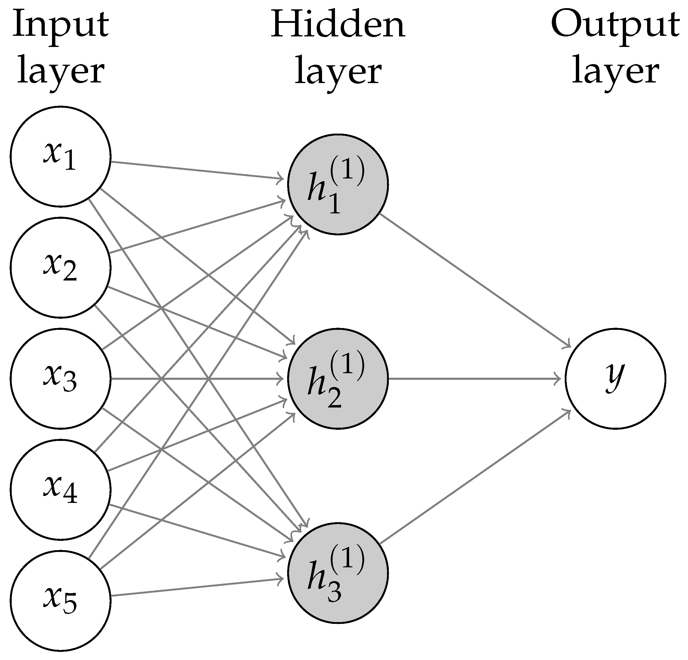
Neural networks (NN) are a widely used tool for predictive purposes. They are intensely used in the Big Data and deep-learning fields, where datasets comprise vast amounts of both variables and observations, and there is the need to fit a predictive model. A typical neural network is composed of an input layer (with the explanatory variables), an output layer (with the response variables; it might contain more than one), and a certain number of hidden layers, which are placed between the input and the output layer (see Figure 3). At each layer, every variable is connected to all the variables in the previous layer. Every hidden node transforms its several inputs into a single output value P according to a specific transfer or propagation function (typically a nonlinear transformation), so that . This propagation function depends on a number of parameters (called weights). Once these weights have been learned for every node with the training dataset, the neural network can be used for making predictions on new data.
In our experiments, we used the R package neuralnet [54] with a single hidden layer containing three hidden nodes (these models are often referred to as multilayer perceptrons, see Figure 3), and made five replications with different random initializations of the weights. We chose these parameters by trial and error; using a larger number of hidden nodes often caused convergence issues in the learning algorithm and might lead to overfitting as well.
2.3.4. Bayesian Networks
Bayesian networks (BNs) are compact representations of the joint probability distribution over a set of variables whose independence relations are encoded by the structure of an underlying directed acyclic graph (DAG) [55]. Formally, a BN is defined as a pair (, ), where is a DAG and is a set of conditional probability distributions (CPDs). is composed of nodes that represent random variables (X) and links between pairs of nodes, representing statistical dependence between them. Each node has a distribution attached, where represents the parents of in . The joint probability distribution over all the variables in the network is defined as the product of the CPDs attached to each node, that is:
where represents the set of all possible values of variable .
There are different ways to represent CPDs, including conditional probability tables (CPTs), conditional linear Gaussian, or Mixtures of Truncated Basis Functions (MoTBFs). In this work, we have used a particular case of MoTBFs [56] called Mixtures of Truncated Exponentials (MTEs) [57], implemented in the Elvira software [58].
A BN can be used as a regression model by computing the conditional expectation of Y given the observed explanatory variables, i.e., . Therefore, conditional density is computed in order to obtain the numerical prediction for Y, which means that the regression model is [59]:
Typically, when facing regression problems only restricted network structures are considered since they reduce the number of parameters to be estimated from data. The extreme case is the naive Bayes (NB) structure, where all explanatory variables X are considered independent given Y (Figure 4a). The independence assumption can be relaxed by expanding the NB structure, i.e., if more dependencies between the variables are considered. Tree-augmented naive Bayes (TAN) models allow each feature to have one more parent besides Y (Figure 4b). The increase in complexity, in both structure and parameter learning, usually results in richer and more accurate models. In this work, we have included both the NB and the TAN models in the comparison of methods.
2.4. Variable Selection
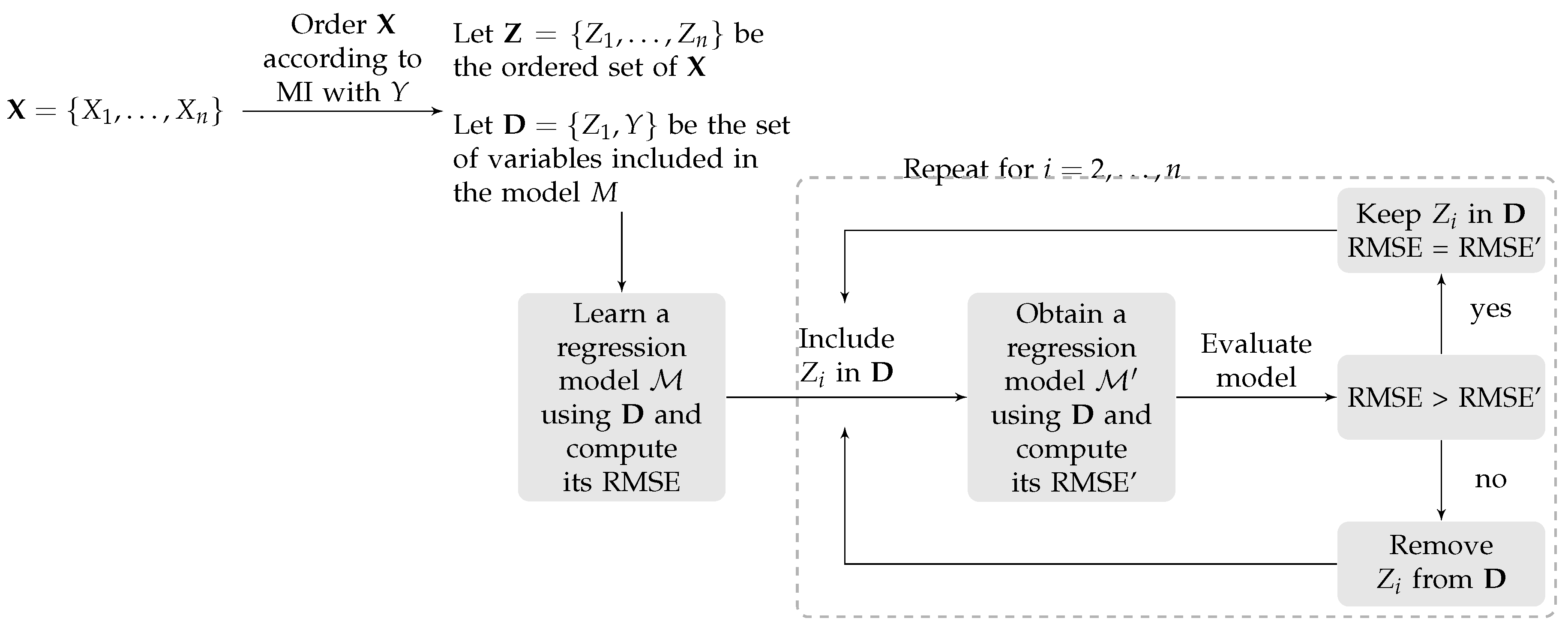
For all the methods, we followed a filter-wrapper variable selection procedure. Firstly, this approach orders explanatory variables according to their mutual information (MI) with response variable Y, obtaining an ordered set . Then, the first variable in () and the response Y are used to learn a regression model. Afterward, the remaining explanatory variables in are inserted in the model, one by one, according to the aforementioned order, and a new regression model is obtained. Whenever the inclusion of a variable increases the accuracy of the model, it is kept; otherwise, it is excluded from the model. The accuracy of the model is measured in terms of its root mean squared error (RMSE), defined as:
Figure 5 shows a graphical representation of the variable selection procedure followed.
2.5. Model Validation
The models were validated employing the k-fold cross-validation technique [60], obtaining a measure of error in each fold. This technique randomly splits the complete dataset into k subsets, using k-1 for learning (train set) and the other for validation (test set). The method is repeated k times so that each time a new train set is used to learn the model and a new test set is used to compute the RMSE. The average of the k error measures gives an estimate of the out-of-sample error. Figure 6 shows a schematic representation of the k-fold cross-validation technique. In our experiments, a k-value of 10 was applied. The 10 RMSE measures of the five aforementioned regression models were compared using Friedman’s Test with maxT statistics [61]. In those cases where significant differences were found, we deployed Wilcoxon–Nemenyi–McDonald-Thompson’s posthoc test [62] to make a pairwise comparison of the methods.
3. Results
Table 3 shows the variables selected by each method. It can be noted that the number of selected variables is higher when the models were learned using the 5 × 5 km grid dataset. In the case of MLR, NB, and TAN, the selected number of variables is twice as high in the grid dataset than in the municipality one. Moreover, we computed the Fleiss kappa measure [63] to evaluate the degree of agreement of the different models at selecting variables, and obtained for the municipality dataset and for the grid dataset, which means that there is a higher degree of agreement in the selection of variables when the models were learned using the municipality dataset.
On a municipality scale, all models selected Population density (pDens) and Distance to the main city (DMC) variables (Table 3). By contrast, the variable Population growth rate (EGR) was only selected by MLR model; the variables Unemployment rate (UR) and Tertiary sector (sect.T) were only selected by the MT model, and Mortality rate (MortR) was only selected by NB. NN selected the same variables as the models based on uncertainty, except for Old-age dependency index (ODI), Mortality rate (MortR), and No studies (st.no). These variables selected by uncertainty models can be representatives of the social characteristics of upland municipalities.
On a 5 × 5 grid scale, the number of variables selected ranged from nine (by Neural Networks) to 18 (by NB model). All models selected the variable Distance to the main city (DMC). The variables Population density (pDens), Sex ratio (SxR), Doubling time (DT), Population growth rate (EGR), Mortality rate (MortR), University (st.uni), and Tertiary sector (sec.T) were selected at least by four models. The variable Illiterate (st.ill) was only selected by TAN model.
A 10-fold cross-validation was carried out in order to test the predictive performance of the five regression models. Table 4 shows the RMSE measures obtained from the 10-fold cross-validation for each model and dataset. It is noticeable that the error is generally lower when the models were learned using the municipality dataset. The 10 RMSE measures of each model were compared to detect statistically significant differences. Figure 7 summarizes the results of the posthoc analysis carried out after the Friedman test. The box plots represent the difference in RMSE values between the corresponding models.
For the sake of understanding, Figure 7 is explained in a simplified fashion. Let A be the set of k RMSE values obtained from model , B the set of k RMSE values corresponding to model and D the set of k values corresponding to the difference between A and B. The box plots in Figure 7 represent D, so that whenever , with , the corresponding point in the box plot is below 0 (horizontal dashed line), which means that model has a lower RMSE, since →, i.e., model predicts better than model in that particular fold. If model systematically outperforms model , then the entire box plot is below 0. Equivalently, whenever , the corresponding point in the box plot is above 0, which means that model has higher RMSE since →, i.e., model predicts worse than model in that particular fold. If model systematically outperforms model , then the entire box plot is above 0.
It can be noted that the statistical test applied did not detect any significant difference (p-value > 0.05) between the models when they were learned using the municipality dataset (Figure 7a). On the other hand, we found significant differences (p-value < 0.05) between 4 pairs of models when they were learned using the grid dataset (Figure 7b). The differences are found between MT-MLR, with the former having a lower error, NB-MT, with the former having a higher error, TAN-MT, with the former having a higher error, and TAN-NN, with the former having a higher error.
Table 5 shows the execution time of the different models for both datasets. MLR is the fastest method, followed by the model tree (MT). On the other hand, the NN and the TAN models were the most time-consuming methods.
4. Discussion
4.1. Models Comparison
An MLR model is a mathematical tool for learning a model from data and making predictions afterward. However, the linear behavior in the data that this model assumes is rarely found in complex environments as the one studied in this paper. In ecology and environmental sciences, multiple regression has been frequently used in predictive modeling [10,11]. It is a simple method based on the linear and additive associations of the explanatory variables, but the colinearity between the independent variables can lead to incorrect identification of the most critical predictors [11]. If we consider cultural landscapes as socioecological systems, this tool should be used carefully, taking into account the nonlinear dynamics of the systems and the restrictions of the model.
On the contrary, MT is much more flexible than MLR [52]. It can adjust to complex data, splitting them into different chunks or pieces according to the values of some variables, and fitting an MLR on every leaf. MT can be understood as a piecewise multiple linear regression model. This makes these models rather adaptable and accurate with respect to learning errors [64]. Nevertheless, they have some significant inconveniences that have to be taken into account. Models involving trees are prone to overfitting, especially when the number of branches in the tree is large [65]. This means that, even if the fitting error is low, the predictions given by these models can be inexact. Additionally, the splitting criteria on the trees may involve thresholds with unnatural values or low-importance variables. This, along with the fact that the MLRs on the leaves of an MT are built with different subsets of variables (related or not with those that appear in the splitting criteria), makes medium- or large-size model trees hardly interpretable.
Even though NN often provide good results in regression problems (in terms of accuracy) [39,64], they require a computationally costly adjustment process in comparison to other methods. Due to their complex multilayer structure, these models are also difficult to interpret. Other problems that arise with the use of neural networks are the choices of their free parameters [35,36], These include the transfer function and the structural parameters (number of hidden layers, and amount of variables in each of them). Another issue is the stochastic nature of the fitting algorithm, which starts with a random guess of the weights, and thus several replications provide different models [36]. It is also known that, for small datasets, other, simpler regression models often outperform NNs, so that neural networks require large datasets to exhibit their advantages. Last but not least, neural networks can be extremely complex models, even with a small size [38]. This can also lead to overfitting if only one focuses on the fitting error.
BNs provide a well-founded approach for dealing with complex systems [44]. The graphical representation provided by BNs makes them a transparent tool, since the different parts of the ecosystem can be seen as nodes that interact with other nodes in a network, and the relationship between them can be mathematically modeled [4,21]. BNs provide not only a numeric prediction of the response but also a full specification of the posterior probability distribution. Knowing this distribution can be useful in practice for making inferences about the response variable as, for instance, computing confidence intervals or testing hypotheses [48,49]. Another advantage is that there is no need to know the value of every explanatory variable to predict the value of the response, making this tool suitable for establishing scenarios of change where only a few variables are involved.
4.2. Socioeconomic Variables as Indicators
The results show that the number of variables selected when the models were built using the municipality dataset differs from the case in which the 5 × 5 grid dataset was used. The Fleiss kappa measure indicates that the selection of socioeconomic indicators using the municipality scale can be more appropriate since there is a higher agreement among the methods. Moreover, the information collected in the 5 × 5 grid may not be as useful since the value taken by each variable in each cell was obtained by weight averaging the data from the municipality scale. Thus, this conversion led to repeated information. For this reason, the discussion is focused on the municipality scale.
- Population density (pDens) and Distance to the main city (DMC) can be considered as the most important indicators since all models selected them. Both variables can be related to land abandonment. The remoteness from big cities, where better connectivity to other cities and accessibility to public services are found, can be relevant factors of land abandonment [66]. Traditionally, emigration has abundantly occurred in cultural landscapes in Andalusia [67], especially among young people and women who seek to acquire a higher education level and better job opportunities in larger cities.
- In the past decades, these landscapes have attracted tourism [68]. The growth of tourism has changed the socioeconomic sectors, developing the tertiary (sec.T identified by the MT model) and hospitality sectors (sec.H). These sectors coexist with the primary sector through agriculture. In this sense, some authors [66,69] consider that many rural areas maintain symbiosis between tourism and agriculture. The variables related to tourism (sec.H) and agriculture (sec.P) were selected by the NN and NB models. Tourism is involved in population growth and the improvement of transportation infrastructures, such as roads [70], attenuating the abandonment process, and giving rural residents an opportunity to enhance their wellbeing [71].
- The variable related to middle-school studies (st.mid) can be considered as an important indicator since it was selected by four out of five models. Generally speaking, people with basic knowledge of writing and reading (st.no), and with middle school being their maximum level of attained education (st.mid), predominate in these landscapes. These variables emphasize the tourism–agriculture relationship. People dedicated to agriculture have basic knowledge, and people dedicated to tourism have middle professional training.
- Sex ratio (SxR) was selected by the MT and TAN models. As aforementioned, plenty of the emigrants are women who aim at obtaining a high education level and better job opportunities. As a consequence, the sex ratio is imbalanced toward men. This tendency is one of the main factors to the social and demographic sustainability of rural landscapes in Spain [70].
5. Conclusions
The applied statistical test did not find significant differences among the models, which means that all of them were competitive from a predictive accuracy point of view. However, they showed other advantages/disadvantages that should be considered when building a model. The main disadvantage of MLR is the linearity assumption, with simplicity and speed being within its advantages. On the other hand, MTs overcome linearity assumptions by splitting the domain of the variables, obtaining more accurate results at the expense of making them hardly interpretable. NNs lack in interpretability and are time-consuming; however, these disadvantages can be accepted if a large dataset is available and the only concern is predictive accuracy. Finally, BNs provide many advantages, with transparency, interpretability, and potential inclusion of expert knowledge being especially relevant in the context of decision-making.
The comparison of these methods revealed some indicators of cultural landscapes that should be taken into account by decision-makers when planning policies or interventions to be implemented at the municipality scale. The management of cultural landscapes has traditionally considered environmental features. Since cultural landscapes are socioecological systems, this management should be done from an integrated perspective, including socioeconomic indicators. The indicators selected in this paper could be used in an integrated policy on cultural-landscape management in Andalusia. In general, the available socioeconomic information is limited to the municipality scale, making it difficult to obtain reliable results when artificially increasing spatial resolution, as shown in the results obtained by the grid dataset. Therefore, it is necessary that public administrations provide socioeconomic information in a higher level of detail. Possible future work in the land planning and management field is to characterize socioecological sectors within cultural landscapes according to the socioeconomic indicators selected in this paper.
Author Contributions
Conceptualization, P.A.A.; methodology, A.D.M. and D.R.-L.; software, A.D.M. and D.R.-L.; validation, A.D.M., D.R.-L., and P.A.A.; formal analysis, A.D.M. and D.R.-L.; investigation, A.D.M., D.R.-L., and P.A.A.; writing—original draft preparation, A.D.M., D.R.-L., and P.A.A.; supervision, A.D.M., D.R.-L., and P.A.A.
Funding
This work has been partly supported by the Spanish Ministry of Economy and Competitiveness, through project TIN2016-77902-C3-3-P.
Acknowledgments
D.R.-L. thanks the support from CDTIME (University of Almería), the research group FQM-229, and from the Campus de Excelencia Internacional del Mar (CEIMAR) of the University of Almería.
Conflicts of Interest
The authors declare no conflict of interest.
References
- Farina, A. The cultural landscape as a model for the integration of ecology and economics. Biosciences 2000, 50, 313–320. [Google Scholar] [CrossRef]
- Plieninger, T.; Bieling, C. Resilience and the Cultural Landscape: Understanding and Managing Change in Human-Shaped Environments; Cambridge University Press: Cambridge, UK, 2012. [Google Scholar]
- Schmitz, M.F.; De Aranzabal, I.; Aguilera, P.A.; Rescia, A.; Pineda, F.D. Relationship between landscape typology and socioeconomic structure: Scenarios of change in Spanish cultural landscapes. Ecol. Model. 2003, 168, 343–356. [Google Scholar] [CrossRef]
- Maldonado, A.D.; Aguilera, P.A.; Salmerón, A.; Nicholson, A.E. Probabilistic modeling of the relationship between socioeconomy and ecosystem services in cultural landscapes. Ecosyst. Serv. 2018. [Google Scholar] [CrossRef]
- De Aranzabal, I.; Schmitz, M.F.; Aguilera, P.; Pineda, F.D. Modelling of landscape changes derived from the dynamics of socio-ecological systems: A case of study in a semiarid Mediterranean landscape. Ecol. Indic. 2008, 8, 672–685. [Google Scholar] [CrossRef]
- Rescia, A.; Willaarts, B.; Schmitz, M.; Aguilera, P. Changes in land uses and management in two Nature Reserves in Spain: Evaluating the social-ecological resilience of natural landscapes. Landsc. Urban Plan. 2010, 98, 26–35. [Google Scholar] [CrossRef]
- Rescia, A.; Pérez-Corona, M.E.; Arribas-Ureña, P.; Dover, J. Cultural landscapes as complex adaptive systems: The cases of northern Spain and Northern Argentina. In Resilience and the Cultural Landscape: Understanding and Managing Change in Human-Shaped Environments; Pleninger, T., Bieling, T., Eds.; Cambridge University Press: Cambridge, UK, 2012; pp. 126–145. [Google Scholar]
- Parrott, L.; Quinn, N. A complex systems approach for multiobjective water quality regulation on managed wetland landscapes. Ecosphere 2016, 7, e01363. [Google Scholar] [CrossRef] [Green Version]
- Parrott, L. Hybrid modelling of complex ecological systems for decision support: Recent successes and future perspectives. Ecol. Inform. 2011, 6, 44–49. [Google Scholar] [CrossRef]
- Guisan, A.; Zimmermann, N.E. Predictive habitat distribution models in ecology. Ecol. Model. 2000, 135, 147–186. [Google Scholar] [CrossRef]
- Sousa, S.; Martins, F.; Alvim-Ferraz, M.; Pereira, M. Multiple linear regression and artificial neural networks based on principal components to predict ozone concentrations. Environ. Model. Softw. 2007, 22, 97–103. [Google Scholar] [CrossRef]
- Banos-Gonzalez, I.; Martínez-Fernández, J.; Esteve-Selma, M.Á.; Esteve-Guirao, P. Sensitivity analysis in socio-ecological models as a tool in environmental policy for sustainability. Sustainability 2018, 10, 2928. [Google Scholar] [CrossRef]
- Bishop, C.M. Pattern Recognition and Machine Learning; Springer: Berlin, Germany, 2006. [Google Scholar]
- Murphy, K. Machine Learning: A Probabilistic Perspective; Adaptive Computation and Machine Learning; MIT Press: Cambridge, MA, USA, 2012. [Google Scholar]
- Valletta, J.J.; Torney, C.; Kings, M.; Thornton, A.; Madden, J. Applications of machine learning in animal behaviour studies. Anim. Behav. 2017, 124, 203–220. [Google Scholar] [CrossRef]
- Kamenova, S.; Bartley, T.; Bohan, D.; Boutain, J.; Colautti, R.; Domaizon, I.; Fontaine, C.; Lemainque, A.; Viol, I.L.; Mollot, G.; et al. Chapter Three - Invasions Toolkit: Current Methods for Tracking the Spread and Impact of Invasive Species. In Networks of Invasion: A Synthesis of Concepts; Bohan, D.A., Dumbrell, A.J., Massol, F., Eds.; Academic Press: Cambridge, MA, USA, 2017; Volume 56, pp. 85–182. [Google Scholar] [CrossRef]
- Aguilera, P.A.; Fernández, A.; Reche, F.; Rumí, R. Hybrid Bayesian network classifiers: Application to species distribution models. Environ. Model. Softw. 2010, 25, 1630–1639. [Google Scholar] [CrossRef]
- Li, X.; Wang, Y. Applying various algorithms for species distribution modelling. Integr. Zool. 2013, 8, 124–135. [Google Scholar] [CrossRef] [PubMed]
- Maldonado, A.D.; Aguilera, P.A.; Salmerón, A. Modeling zero-inflated explanatory variables in hybrid Bayesian network classifiers for species occurrence prediction. Environ. Model. Softw. 2016, 82, 31–43. [Google Scholar] [CrossRef]
- Tamaddoni-Nezhad, A.; Milani, G.A.; Raybould, A.; Muggleton, S.; Bohan, D.A. Chapter Four—Construction and Validation of Food Webs Using Logic-Based Machine Learning and Text Mining. In Ecological Networks in an Agricultural World; Woodward, G., Bohan, D.A., Eds.; Academic Press: Cambridge, MA, USA, 2013; Volume 49, pp. 225–289. [Google Scholar] [CrossRef]
- Uusitalo, L.; Tomczak, M.T.; Müller-Karulis, B.; Putnis, I.; Trifonova, N.; Tucker, A. Hidden variables in a Dynamic Bayesian Network identify ecosystem level change. Ecol. Inform. 2018, 45, 9–15. [Google Scholar] [CrossRef]
- Willcock, S.; Martínez-López, J.; Hooftman, D.A.; Bagstad, K.J.; Balbi, S.; Marzo, A.; Prato, C.; Sciandrello, S.; Signorello, G.; Voigt, B.; et al. Machine learning for ecosystem services. Ecosyst. Serv. 2018, 33, 165–174. [Google Scholar] [CrossRef]
- Zickus, M.; Greig, A.J.; Niranjan, M. Comparison of Four Machine Learning Methods for Predicting Pm 10 Concentrations in Helsinki, Finland. Water Air Soil Pollut. 2002, 2, 717–729. [Google Scholar] [CrossRef]
- Chen, G.; Li, S.; Knibbs, L.D.; Hamm, N.; Cao, W.; Li, T.; Guo, J.; Ren, H.; Abramson, M.J.; Guo, Y. A machine learning method to estimate PM2.5 concentrations across China with remote sensing, meteorological and land use information. Sci. Total Environ. 2018, 636, 52–60. [Google Scholar] [CrossRef] [PubMed]
- Martínez-España, R.; Bueno-Crespo, A.; Timón, I.; Soto, J.; Muñoz, A.; Cecilia, J.M. Air-Pollution Prediction in Smart Cities through Machine Learning Methods: A Case of Study in Murcia, Spain. J. Univ. Comput. Sci. 2018, 24, 261–276. [Google Scholar]
- Aguilera, P.A.; Fernández, A.; Ropero, R.F.; Molina, L. Groundwater quality assessment using data clustering based on hybrid Bayesian networks. Stoch. Environ. Res. Risk Assess. 2013, 27, 435–447. [Google Scholar] [CrossRef]
- Sajedi-Hosseini, F.; Malekian, A.; Choubin, B.; Rahmati, O.; Cipullo, S.; Coulon, F.; Pradhan, B. A novel machine learning-based approach for the risk assessment of nitrate groundwater contamination. Sci. Total Environ. 2018, 644, 954–962. [Google Scholar] [CrossRef]
- Vesselinov, V.V.; Alexandrov, B.S.; O’Malley, D. Contaminant source identification using semi-supervised machine learning. J. Contam. Hydrol. 2018, 212, 134–142. [Google Scholar] [CrossRef] [PubMed]
- Belanche-Muñoz, L.; Blanch, A.R. Machine learning methods for microbial source tracking. Environ. Model. Softw. 2008, 23, 741–750. [Google Scholar] [CrossRef]
- Kim, Y.H.; Im, J.; Ha, H.K.; Choi, J.K.; Ha, S. Machine learning approaches to coastal water quality monitoring using GOCI satellite data. GISci. Remote Sens. 2014, 51, 158–174. [Google Scholar] [CrossRef]
- Maldonado, A.D.; Aguilera, P.A.; Salmerón, A. Continuous Bayesian networks for probabilistic environmental risk mapping. Stoch. Environ. Res. Risk Assess. 2016, 30, 1441–1455. [Google Scholar] [CrossRef]
- Karpatne, A.; Jiang, Z.; Vatsavai, R.R.; Shekhar, S.; Kumar, V. Monitoring Land-Cover Changes: A Machine-Learning Perspective. IEEE Geosci. Remote Sens. Mag. 2016, 4, 8–21. [Google Scholar] [CrossRef]
- Maclaurin, G.J.; Leyk, S. Temporal replication of the national land cover database using active machine learning. GISci. Remote Sens. 2016, 53, 759–777. [Google Scholar] [CrossRef]
- Gibril, M.B.A.; Idrees, M.O.; Shafri, H.Z.M.; Yao, K. Integrative image segmentation optimization and machine learning approach for high quality land-use and land-cover mapping using multisource remote sensing data. J. Appl. Remote Sens. 2018, 12, 016036. [Google Scholar] [CrossRef]
- LeCun, Y.; Bengio, Y.; Hinton, G. Deep learning. Nature 2015, 521, 436–444. [Google Scholar] [CrossRef] [PubMed]
- Schmidhuber, J. Deep learning in neural networks: An overview. Neural Netw. 2015, 61, 85–117. [Google Scholar] [CrossRef] [PubMed] [Green Version]
- Specht, D.F. A General Regression Neural Network. IEEE Trans. Neural Netw. 1991, 2, 568–576. [Google Scholar] [CrossRef] [PubMed]
- Larochelle, H.; Bengio, Y.; Louradour, J.; Lamblin, P. Exploring Strategies for Training Deep Neural Networks. J. Mach. Learn. Res. 2009, 10, 1–40. [Google Scholar]
- Zhang, G.; Patuwo, B.E.; Hu, M.Y. Forecasting with artificial neural networks: The state of the art. Int. J. Forecast. 1998, 14, 35–62. [Google Scholar] [CrossRef]
- Ciregan, D.; Meier, U.; Schmidhuber, J. Multi-column deep neural networks for image classification. In Proceedings of the 2012 IEEE Conference on Computer Vision and Pattern Recognition, Providence, RI, USA, 16–21 June 2012; pp. 3642–3649. [Google Scholar] [CrossRef]
- Collobert, R.; Weston, J. A Unified Architecture for Natural Language Processing: Deep Neural Networks with Multitask Learning. In Proceedings of the ICML ’08 25th International Conference on Machine Learning, Helsinki, Finland, 5–9 July 2008; ACM: New York, NY, USA, 2008; pp. 160–167. [Google Scholar] [CrossRef]
- Kohara, K.; Ishikawa, T.; Fukuhara, Y.; Nakamura, Y. Stock Price Prediction Using Prior Knowledge and Neural Networks. Intell. Syst. Account. Financ. Manag. 1997, 6, 11–22. [Google Scholar]
- Ghahramani, Z. Probabilistic machine learning and artificial intelligence. Nature 2015, 521, 452–459. [Google Scholar] [CrossRef] [PubMed]
- Koller, D.; Friedman, N. Probabilistic Graphical Models: Principles and Techniques; Adaptive Computation and Machine Learning; The MIT Press: Cambridge, MA, USA, 2009. [Google Scholar]
- Ramos-López, D.; Masegosa, A.R.; Martínez, A.M.; Salmerón, A.; Nielsen, T.D.; Langseth, H.; Madsen, A.L. MAP inference in dynamic hybrid Bayesian networks. Prog. Artif. Intell. 2017, 6, 133–144. [Google Scholar] [CrossRef] [Green Version]
- Masegosa, A.; Nielsen, T.D.; Langseth, H.; Ramos-López, D.; Salmerón, A.; Madsen, A.L. Bayesian Models of Data Streams with Hierarchical Power Priors. In Proceedings of the 34th International Conference on Machine Learning, Sydney, Australia, 6–11 August 2017; Precup, D., Teh, Y.W., Eds.; PMLR, International Convention Centre: Sydney, Australia, 2017; Volume 70, pp. 2334–2343. [Google Scholar]
- Jordan, M.I. Graphical Models. Stat. Sci. 2004, 19, 140–155. [Google Scholar] [CrossRef]
- Nasrabadi, N.M. Pattern Recognition and Machine Learning. J. Electron. Imaging 2007, 16, 049901. [Google Scholar] [CrossRef] [Green Version]
- Larrañaga, P.; Moral, S. Probabilistic graphical models in artificial intelligence. Appl. Soft Comput. 2011, 11, 1511–1528. [Google Scholar] [CrossRef]
- Olea, L.; San Miguel-Ayanz, A. The Spanish dehesa. A traditional Mediterranean silvopastoral system linking production and nature conservation. In Proceedings of the 21st General Meeting of the European Grassland Federation, Badajoz, Spain, 3–6 April 2006. [Google Scholar]
- R Development Core Team. R: A Language and Environment for Statistical Computing; R Foundation for Statistical Computing: Vienna, Austria, 2012; ISBN 3-900051-07-0. [Google Scholar]
- Wang, Y.; Witten, I.H. Induction of model trees for predicting continuous cases. In Proceedings of the Poster Papers of the European Conference on Machine Learning, Prague, Czech Republic, 23–25 April 1997; pp. 128–137. [Google Scholar]
- Hornik, K.; Buchta, C.; Zeileis, A. Open-Source Machine Learning: R Meets Weka. Comput. Stat. 2009, 24, 225–232. [Google Scholar] [CrossRef]
- Günther, F.; Fritsch, S. neuralnet: Training of Neural Networks. R J. 2010, 2, 30–38. [Google Scholar]
- Pearl, J. Probabilistic Reasoning in Intelligent Systems; Morgan-Kaufmann (San Mateo): San Francisco, CA, USA, 1988. [Google Scholar]
- Langseth, H.; Nielsen, T.D.; Rumí, R.; Salmerón, A. Mixtures of Truncated Basis Functions. Int. J. Approx. Reason. 2012, 53, 212–227. [Google Scholar] [CrossRef]
- Moral, S.; Rumí, R.; Salmerón, A. Mixtures of Truncated Exponentials in Hybrid Bayesian Networks. In Symbolic and Quantitative Approaches to Reasoning with Uncertainty; Benferhat, S., Besnard, P., Eds.; Springer: Berlin, Germany, 2001; Volume 2143, pp. 156–167. [Google Scholar]
- Elvira Consortium. Elvira: An Environment for Creating and Using Probabilistic Graphical Models. In Proceedings of the First European Workshop on Probabilistic Graphical Models, Cuenca, Spain, 6–8 November 2002; pp. 222–230. [Google Scholar]
- Fernández, A.; Salmerón, A. Extension of Bayesian network classifiers to regression problems. In Advances in Artificial Intelligence—IBERAMIA 2008; Geffner, H., Prada, R., Alexandre, I.M., David, N., Eds.; Springer: Berlin, Germany, 2008; Volume 5290, pp. 83–92. [Google Scholar]
- Stone, M. Cross-Validatory Choice and Assessment of Statistical Predictions. J. R. Stat. Soc. Ser. B 1974, 36, 111–147. [Google Scholar]
- Hothorn, T.; Hornik, K.; van de Wiel, M.; Zeileis, A. Implementing a Class of Permutation Tests: The coin Package. J. Stat. Softw. 2008, 28, 1–23. [Google Scholar] [CrossRef]
- Hollander, M.; Wolfe, D.A. Nonparametric Statistical Methods, 2nd ed.; Wiley: Hoboken, NJ, USA, 1999. [Google Scholar]
- Fleiss, J.L. Measuring nominal scale agreement among many raters. Psychol. Bull. 1971, 76, 378–382. [Google Scholar] [CrossRef]
- Bhattacharya, B.; Solomatine, D. Neural networks and M5 model trees in modelling water level—Discharge relationship. Neurocomputing 2005, 63, 381–396. [Google Scholar] [CrossRef]
- Perlich, C.; Provost, F.; Simonoff, J.S. Tree induction vs. logistic regression: A learning-curve analysis. J. Mach. Learn. Res. 2003, 4, 211–255. [Google Scholar]
- Vidal-Macua, J.J.; Ninyerola, M.; Zabala, A.; Domingo-Marimon, C.; Gonzalez-Guerrero, O.; Pons, X. Environmental and socioeconomic factors of abandonment of rainfed and irrigated crops in northeast Spain. Appl. Geogr. 2018, 90, 155–174. [Google Scholar] [CrossRef]
- Rey Benayas, J.M.; Martins, A.; Nicolau, J.M.; Schulz, J.J. Abandonment of agricultural land: An overview of drivers and consequences. CAB Rev. Perspect. Agric. Vet. Sci. Nutr. Nat. Resour. 2007, 2, 1–14. [Google Scholar] [CrossRef]
- Schmitz, M.F.; Pineda, F.D.; Castro, H.; De Aranzabal, I.; Aguilera, P. Paisaje Cultural y Estructura SocioeconóMica. Valor Ambiental y Demanda TuríStica en un Territorio MediterráNeo; Junta de Andalucía: Sevilla, Spain, 2005. [Google Scholar]
- Cánoves, G.; Villarino, M.; Priestley, G.K.; Blanco, A. Rural tourism in Spain: An analysis of recent evolution. Geoforum 2004, 35, 755–769. [Google Scholar] [CrossRef]
- Consejo Económico y Social de España (CES). El Medio Rural y su VertebracióN Social y Territorial; Colección Informes: Madrid, Spain, 2018. [Google Scholar]
- Muresan, I.C.; Oroian, C.F.; Harun, R.; Arion, F.H.; Porotiu, A.; Chiciudean, G.; Todea, A.; Lile, R. Local Residents’ Attitude toward sustainable rural tourism development. Sustainability 2016, 8, 100. [Google Scholar] [CrossRef]
Figure 1.
The region of Andalusia divided into its four main geomorphological units (a). Study area is focused on the cultural landscapes of Andalusia, which are mainly located in the Baetic System and the Sierra Morena mountain range. (b,c) Units of analysis: the municipality and the 5 × 5 km grid, respectively.

Figure 2.
Example of a model tree with six explanatory variables () and five leaves.

Figure 3.
Example of a neural network (multilayer perceptron) with five input variables (), a single hidden layer with three nodes (), and a single output variable (Y). The weights and propagation function have been omitted here for the sake of clarity.
Figure 3.
Example of a neural network (multilayer perceptron) with five input variables (), a single hidden layer with three nodes (), and a single output variable (Y). The weights and propagation function have been omitted here for the sake of clarity.

Figure 4.
Examples of directed acyclic graphs (DAGs) in a Bayesian network with four explanatory variables. Left: a naive Bayes (NB) model. Right: a tree-augmented naive Bayes (TAN) model.
Figure 4.
Examples of directed acyclic graphs (DAGs) in a Bayesian network with four explanatory variables. Left: a naive Bayes (NB) model. Right: a tree-augmented naive Bayes (TAN) model.

Figure 5.
Algorithm for variable selection.

Figure 6.
Schematic representation of k-fold cross-validation.

Figure 7.
Box plots of the difference in model performance between pairs of models with regards to RMSE for both the (a) municipality and (b) grid datasets. Boxes filled in red indicate significant differences between the corresponding models according to the posthoc analysis carried out after the Friedman test.


Table 1.
Data description.
| Variable Name (Code) | Definition |
|---|---|
| Heterogeneous land (HET) | Percentage of heterogeneous lands, obtained as the combination of (1) patches of mixing grassland and forest and (2) crops with natural vegetation, from the Land use and land cover map of Andalusia of 2011 (at scale 1:10,000), based on the Land Occupation Information System of Spain (SIOSE). |
| Population density (pDens) | Population density of each municipality in 2011 (inhabitants/Km). |
| Sex ratio (SxR) | Proportion of males (M) to females (F) in each municipality in 2011, computed as . |
| Doubling time (DT) | Time (in years) the population takes to double or reduce to half its size, computed as , where r is the population growth rate. |
| Human Development Index (HDI) | Well-being in a population in terms of life expectancy, knowledge and standards of living, computed as , where LE is the Life expectancy index, EI is the Education index and II is the Income index. Variables LE, EI and II are described in Table 2. |
| Distance to main city (DMC) | Distance (Km) from the main settlement in a municipality to the nearest urban settlement with more than 50,000 inhabitants. |
| Population growth rate (EGR) | Exponential growth of the population, computed as , where represents the population in 2001, the population in 2011 and t the 10-year period. |
| Old-age dependency index (ODI) | Percentage of the older over the younger population in 2011, computed as , where is the population older than 65 years old and is the population younger than 15 years old. |
| Index of Migration effectiveness (IME) | Percentage of total migration for the period 2001–2011. It ranges from −100 (emigration) to 100 (immigration), with values close to 0 indicating no change in the population dynamic. It is computed as . |
| Mortality rate (MortR) | Number of deaths per 1000 inhabitants in each municipality in 2011. |
| Birth rate (BirthR) | Number of births per 1000 inhabitants in each municipality in 2011. |
| Workforce (WF) | Percentage of the municipality’s working age population (≥16) that are available to work in 2011. It is computed as ; where is the Employment Rate; is the Unemployment Rate and is the population older than 16 years old. |
| Unemployment rate (UR) | Percentage of workforce that is unemployed. |
| Earned income (earnInc) | Income declared (€) per number of declarations in 2011. |
| Illiterate (st.ill) | Number of illiterate people per 1000 inhabitants (computed from people over 16). |
| No studies (st.no) | Number of people who do not have any level of educational attainment but know how to write and read per 1000 inhabitants (computed from people over 16). |
| Elementary school (st.elem) | Number of people whose maximum level of education attained is elementary school per 1000 inhabitants (computed from people over 16). |
| Middle school (st.mid) | Number of people whose maximum level of education attained is middle school per 1000 inhabitants (computed from people over 16). |
| High school (st.high) | Number of people whose maximum level of education attained is high school per 1000 inhabitants (computed from people over 16). |
| University (st.uni) | Number of people whose maximum level of education attained is a university degree per 1000 inhabitants (computed from people over 16). |
| Primary sector (sec.P) | Number of employees in the primary sector per 1000 inhabitants. |
| Secondary sector (sec.S) | Number of employees in the secondary sector per 1000 inhabitants. |
| Hospitality sector (sec.H) | Number of employees in the hospitality sector (hotels and restaurants) per 1000 inhabitants. |
| Tertiary sector (sec.T) | Number of employees in the Freight, Trading, Banking or Service sectors, including business services, education, health care and other social services, per 1000 inhabitants. |
Table 2.
Variables used to compute some variables in Table 1 but not included the models.
Table 2.
Variables used to compute some variables in Table 1 but not included the models.
| Variable Name (Code) | Definition |
|---|---|
| Income index (II) | The Income Index was obtained as , where IPC is the Income Per Capita. It was used to compute the HDI. |
| Education Index (EI) | The Education Index was obtained by weight averaging the Adult Literacy Index (ALI) and the Gross Enrollment Index (GEI) as . It was used to compute the HDI. |
| Life expectancy index (LEI) | It was obtained from the Multiterritorial Information System of Andalusia at the provincial scale (since it should not be computed for small populations due to the introduction of bias). It was used to compute the HDI. |
| Adult Literacy Index | Proportion of people that know how to write and read. It was used to compute the Education Index (EI). |
| Gross Enrollment Index | Proportion of people of age 6 to 25 enrolled in school at levels from elementary school to university. It was used to compute the Education Index (EI). |
| Income Per Capita (IPC) | Total income (€) in a municipality divided by total number of inhabitants in 2011. It was used to compute the Income Index (II). |
Table 3.
Variables selected by each method for both the municipality and the 5 × 5 km grid datasets. MLR: multiple linear regression; MT: model tree; NN: neural network; NB: naive Bayes; TAN: tree augmented naive Bayes.
Table 3.
Variables selected by each method for both the municipality and the 5 × 5 km grid datasets. MLR: multiple linear regression; MT: model tree; NN: neural network; NB: naive Bayes; TAN: tree augmented naive Bayes.
| Municipality Dataset | 5 × 5 Km Grid Dataset | ||||||||||||
|---|---|---|---|---|---|---|---|---|---|---|---|---|---|
| Variables | MLR | MT | NN | NB | TAN | Times Selected | Variables | MLR | MT | NN | NB | TAN | Times Selected |
| pDens | x | x | x | x | x | 5 | pDens | x | x | x | x | 4 | |
| SxR | x | x | 2 | SxR | x | x | x | x | 4 | ||||
| DT | x | x | x | 3 | DT | x | x | x | x | 4 | |||
| HDI | x | x | x | 3 | HDI | x | x | 2 | |||||
| DMC | x | x | x | x | x | 5 | DMC | x | x | x | x | x | 5 |
| EGR | x | 1 | EGR | x | x | x | x | 4 | |||||
| ODI | x | x | 2 | ODI | x | x | 2 | ||||||
| IME | 0 | IME | x | x | 2 | ||||||||
| MortR | x | 1 | MortR | x | x | x | x | 4 | |||||
| BirthR | 0 | BirthR | x | x | 2 | ||||||||
| WF | 0 | WF | x | x | x | 3 | |||||||
| UR | x | 1 | UR | x | x | x | 3 | ||||||
| earnInc | x | x | x | 3 | earnInc | x | x | x | 3 | ||||
| st.ill | 0 | st.ill | x | 1 | |||||||||
| st.no | x | x | 2 | st.no | x | x | 2 | ||||||
| st.elem | 0 | st.elem | x | x | x | 3 | |||||||
| st.mid | x | x | x | x | 4 | st.mid | x | x | x | 3 | |||
| st.high | 0 | st.high | x | x | x | 3 | |||||||
| st.uni | 0 | st.uni | x | x | x | x | 4 | ||||||
| sec.P | x | x | x | 3 | sec.P | x | x | 2 | |||||
| sec.S | x | 1 | sec.S | x | x | 2 | |||||||
| sec.H | x | x | x | x | 4 | sec.H | x | x | 2 | ||||
| sec.T | x | 1 | sec.T | x | x | x | x | 4 | |||||
| Total selected | 8 | 10 | 7 | 9 | 7 | Total selected | 16 | 10 | 9 | 18 | 15 | ||
Table 4.
RMSE obtained in each fold of the 10-fold cross-validation. The mean value of the 10 measures is also shown.
Table 4.
RMSE obtained in each fold of the 10-fold cross-validation. The mean value of the 10 measures is also shown.
| Municipality Dataset | 5 × 5 km Grid Dataset | ||||||||||
|---|---|---|---|---|---|---|---|---|---|---|---|
| MLR | MT | NN | NB | TAN | MLR | MT | NN | NB | TAN | ||
| Fold 1 | 8.80 | 9.12 | 8.71 | 8.90 | 8.40 | Fold 1 | 14.80 | 12.05 | 13.12 | 15.18 | 15.42 |
| Fold 2 | 9.43 | 9.11 | 8.61 | 9.62 | 9.80 | Fold 2 | 13.80 | 12.88 | 12.77 | 13.28 | 13.50 |
| Fold 3 | 11.45 | 10.21 | 12.43 | 11.61 | 11.59 | Fold 3 | 14.73 | 12.18 | 13.75 | 14.66 | 14.27 |
| Fold 4 | 7.90 | 8.05 | 7.88 | 8.35 | 7.76 | Fold 4 | 13.54 | 10.25 | 11.64 | 13.59 | 14.06 |
| Fold 5 | 16.85 | 13.65 | 15.22 | 16.51 | 15.41 | Fold 5 | 16.42 | 13.14 | 14.82 | 16.83 | 17.02 |
| Fold 6 | 11.44 | 8.55 | 9.39 | 10.62 | 11.68 | Fold 6 | 16.38 | 14.18 | 14.70 | 15.86 | 16.60 |
| Fold 7 | 11.66 | 9.28 | 9.46 | 11.95 | 11.98 | Fold 7 | 15.44 | 14.14 | 14.54 | 14.00 | 15.01 |
| Fold 8 | 13.97 | 13.64 | 12.85 | 13.82 | 14.52 | Fold 8 | 17.38 | 15.69 | 15.82 | 17.95 | 18.20 |
| Fold 9 | 10.85 | 9.30 | 8.18 | 11.01 | 10.61 | Fold 9 | 14.07 | 11.42 | 13.59 | 14.28 | 15.10 |
| Fold 10 | 11.23 | 9.75 | 10.94 | 10.02 | 9.89 | Fold 10 | 14.39 | 12.41 | 13.07 | 14.54 | 14.57 |
| Mean | 11.36 | 10.07 | 10.37 | 11.24 | 11.16 | Mean | 15.09 | 12.83 | 13.78 | 15.02 | 15.37 |
Table 5.
Running time of the 10-fold cross-validation for each model.
| Municipality Dataset | 5 × 5 km Grid Dataset | ||||||||||
|---|---|---|---|---|---|---|---|---|---|---|---|
| LR | M5P | NN | NB | TAN | LR | M5P | NN | NB | TAN | ||
| seconds | 0.073 | 0.895 | 196.847 | 50.334 | 260.767 | seconds | 0.114 | 2.359 | 1891.152 | 826.915 | 14,234.235 |
| minutes | 0.001 | 0.015 | 3.281 | 0.839 | 4.346 | minutes | 0.002 | 0.039 | 31.519 | 13.782 | 237.237 |
© 2018 by the authors. Licensee MDPI, Basel, Switzerland. This article is an open access article distributed under the terms and conditions of the Creative Commons Attribution (CC BY) license (http://creativecommons.org/licenses/by/4.0/).
Share and Cite
MDPI and ACS Style
Maldonado, A.D.; Ramos-López, D.; Aguilera , P.A. A Comparison of Machine-Learning Methods to Select Socioeconomic Indicators in Cultural Landscapes. Sustainability 2018, 10, 4312. https://doi.org/10.3390/su10114312
AMA Style
Maldonado AD, Ramos-López D, Aguilera PA. A Comparison of Machine-Learning Methods to Select Socioeconomic Indicators in Cultural Landscapes. Sustainability. 2018; 10(11):4312. https://doi.org/10.3390/su10114312
Chicago/Turabian StyleMaldonado, Ana D., Darío Ramos-López, and Pedro A. Aguilera . 2018. "A Comparison of Machine-Learning Methods to Select Socioeconomic Indicators in Cultural Landscapes" Sustainability 10, no. 11: 4312. https://doi.org/10.3390/su10114312
Note that from the first issue of 2016, this journal uses article numbers instead of page numbers. See further details here.