Container Transport Network for Sustainable Development in South Korea

Abstract

The ever-increasing tendency toward economic globalization highlights the importance of sustainable container transport networks to a country’s international trade, especially for an economy that is highly dependent on exports. This paper aims to develop a transport network connectivity index (TNCI) to measure the container transport connectivity from a multi-modal perspective. The proposed index is based on both graph theory and economics, considering transport infrastructure and capacity, cargo flow, and capacity utilization. Using the case of South Korea as an example, we apply the TNCI to assess the connectivity of the Busan, Gwangyang, and Incheon ports, representing approximately 96% of the container throughput in South Korea. The calculated TNCI not only provides insight into the assessment of sustainable port competitiveness, it also helps policymakers identify bottlenecks in multi-modal transport networks. To eliminate these bottlenecks, this paper offers some appropriate measures and specific strategies for port development, which in turn improves the connectivity of container transport networks for sustainable development.

1. Introduction

The tendency toward economic globalization has emphasized world merchandise trade as well as international seaborne trade. According to the Review of Maritime Transport (2017) [1], the volume of international seaborne trade has expanded significantly over the last four decades, rising from 2.61 billion tons in 1970 to 4.01 billion tons in 1990, 8.41 billion tons in 2010, and 10.29 billion tons in 2016. Particularly, as shown in

Table 1. Development of international seaborne trade (millions of tons loaded). Sources: Review of Maritime Transport, 2017, UNCTAD (United Nations Conference on Trade and Development).

Year	Oil and Gas	Main Bulk	Container	Other Dry Cargo
2005	2422	1709	1001	2978
2006	2698	1814	1076	3188
2007	2747	1953	1193	3334
2008	2742	2065	1249	3422
2009	2642	2085	1127	3131
2010	2772	2335	1280	3302
2011	2794	2486	1393	3505
2012	2841	2742	1464	3614
2013	2829	2923	1544	3762
2014	2825	2985	1640	4033
2015	2932	3121	1661	3971
2016	3055	3172	1720	4059

, container trade has also increased from 1001 million tons loaded in 2005 to 1280 million tons loaded in 2010, reaching 1720 million tons loaded in 2016. The ever-increasing volume of seaborne trade drives the demand for maritime transport services, especially for container transport services [2]. When providing container transport services, ports play a substantial role as a cluster of loading, unloading, and transshipment activities, shipbrokers, warehousing, and storage services [3] (pp. 638–655), [4]. In this sense, connectivity between the port and its inland container transport networks has a profound impact on port efficiency and port productivity, as well as on a country’s exports and imports.

When providing container transport services, better port connectivity with inland container transport networks is more likely to reduce transit and transport time, and lower transport costs, thereby decreasing the risk of product damage and ensuring product quality. Meanwhile, products unloaded at a port are likely to be delivered faster to customers, which can increase customer satisfaction with shippers, and consequently lead to positive word-of-mouth from satisfied customers. As a result, better port connectivity with inland container transport networks would enlarge a port’s overall captive area, and thereby enable it to serve larger hinterland markets [5]. This potentially strengthens a port’s efficiency and promotes port development in a sustainable manner. In addition, the local economy can also benefit when ports and inland container transport networks are well-connected. For example, better connectivity usually indicates higher market reachability and accessibility to goods and services, and then potentially reduces local firms’ logistics costs and facilitates their import and export business, shaping a sustainable and healthy economy [6]. Due to the decreased logistics costs, more foreign direct investments could be attracted to the local economy. In contrast, delivery delays and traffic congestions are more likely to occur when poor connectivity among roads, railways, and ports is observed. The congested container transport network can cause significant negative impacts not only on port users and port authorities, but also on local environment and residents [7]. Policymakers need to identify bottlenecks in multi-modal transport networks. By doing so, they can improve the efficiency of transport investments among roads, railways, and ports to achieve a better integration of sustainability in transporting containers. Using container transport in South Korea as a case study, this paper aims to develop a transport network connectivity index (TNCI) to examine how containers are transported from the multi-modal perspective. After considering transport infrastructure and capacity, cargo flow, and capacity utilization, the difference between the link capacity and its cargo flow can be used to evaluate the container transport network connectivity, which enables port users to identify ports that have a better connection with inland container transport networks.

Connectivity is a fundamental concept in graph theory. In a representative graph consisting of nodes, arcs, and flows, a node is a connection point, a redistribution point, or a flow endpoint; an arc is a link between two different nodes reflecting costs, flow limits, or specific conditions; and flow shows the quantity of an object movement, which is described by the sequence of a node and arc where flow passes. Accordingly, connectivity can be defined as the minimum number of elements (nodes or edges) that need to be removed to disconnect the remaining nodes from each other [8] (p. 173). Since a graph and a transport network have a lot in common, graph theory has been widely applied in the field of transportation. Specifically, in a transport network, a node generally refers to the cargo-handling facility or origin/destination of cargo; an arc can be a road, railway, sea route, or airway that connects nodes; and a flow usually represents the real cargo movement between two different regions. In this regard, connectivity is redefined as the number of paths or maximum flow quantity between two different nodes in this paper.

In the field of transportation, the air connectivity index (ACI) is a widely known connectivity indicator that seeks to measure the integration in the global air transport network. Using a generalized gravity model, Arvis and Shepherd defined the ACI as the importance of a nation as a node within the global air transport system, and pointed out that the ACI was strongly correlated with the degree of liberalization in air service markets [9]. Apart from the ACI, the liner shipping connectivity index (LSCI) developed by the United Nations Conference on Trade and Development (UNCTD) in 2007 seeks to capture how well nations are connected to global shipping networks. Five components of the maritime transport sector involving the number of ships, their container-carrying capacity, maximum vessel size, number of services, and number of companies that deploy container ships in a nation’s ports are included in the LSCI. Hoffman and Wilmsmeier identified the LSCI and port infrastructure as important determinants of intra-Caribbean freight rates [10]. Additionally, the KOF Swiss Economic Institute published the globalization index to reflect global connectivity, integration, and interdependence in the economic, social, technological, cultural, political, and ecological spheres. A closer inspection of the economic globalization index reveals that two different types of data are involved. One type represents actual flows regarding trade, foreign direct investment (FDI), portfolio investment, and income payments to foreign nationals. The other type represents restrictions, such as hidden import barriers, the mean tariff rate, taxes on international trade, and capital account restrictions [11].

Other popular applications of connectivity are as follows: transit connectivity measuring how equitable the distribution of transit access is in a region [12,13], network connectivity pertaining to the issue of non-motorized transport and university populations [14], cultural heritage connectivity regarding transportation infrastructure planning [15], city connectivity concerning infrastructure networks among 67 important South Asian cities [16], and port connectivity in terms of inter-port relationships from the perspective of a supply chain [17], its impact on the transportation network [18,19], transport costs [20], transit time [21], and transportation access [22].

A more detailed discussion of port connectivity based on the graph theory can be found in [20]. Focusing on degree, betweenness, and port accessibility index, they highlighted the crucial role of port connectivity in keeping transport costs under control. Jiang et al. introduced two models, the minimum transportation time model and the maximum transportation capacity model, to measure port connectivity from a global container liner shipping network perspective [18]. Lam and Yap placed emphasis on shipping capacity, trade routes, and geographic regions, as well as on the extensity and intensity of inter-port relationships among ports [17]. Unlike the aforementioned studies, we focus on transport infrastructure and capacity, cargo flow, and capacity utilization, and derive the TNCI to measure container port connectivity from the multi-modal perspective, rather than from the inter-port perspective. The calculated TNCI not only provides insight into port competitiveness, but also helps policymakers to identify bottlenecks in multi-modal transport networks. After taking appropriate measures, these bottlenecks could be eliminated, which in turn can improve the connectivity of container transport networks in South Korea.

The remainder of this paper is structured as follows. Section 2 presents the potential methodological issues and derives the TNCI. Using the case of South Korea as an example, Section 3 demonstrates data collection and parameter estimations. Section 4 gives a detailed discussion of South Korea’s container transport network connectivity. Finally, relevant conclusions and directions for future research are shown in Section 5.

2. Materials and Methods

Since the multi-modal transport network and the graph theory have a lot in common, it is widely accepted that a transport network can be represented as a graph, and then its connectivity can be examined using the graph theory. Using container transport as an example, a node represents the facility where a container is handled for transit, consolidation, or other specific purposes, while a link denotes the transport infrastructure that connects different nodes through roads/railways. Considering the capacity utilization rate and variance in cargo flow, we can compare the link capacity and the cargo flow to measure connectivity.

Specifically, when the link capacity is smaller than the cargo flow, it is generally believed that roads/railways have been over-utilized, resulting in serious congestion. Then, poor connectivity can be observed in the container transport network. On the other hand, when the link capacity is higher than the cargo flow, the roads/railways have not been fully utilized; the larger the difference between them, the lower the possibility of observing congestion. This can reduce the negative impacts of land transport on environment and then promote the economy in a sustainable manner [23]. In other words, the container transport network is more likely to be well-connected, and better connectivity is likely to be seen. In this regard, the difference between the link capacity and its cargo flow can be regarded as a reasonable evaluation of connectivity, which can be used as a criterion for shipping lines’ port selection.

Before developing the TNCI, some parameters relevant to a multi-modal transport network are defined as follows:

• $N$ set of nodes
• $L$ set of links connecting two different nodes
• $V_{\left(i,j\right)}$ variance in cargo flow from node $i$ to node $j$
• $U_{\left(i,j\right)}$ capacity utilization ratio of link connecting node $i$ and node $j$
• $F_{\left(i,j,t\right)}$ cargo flow from node $i$ to node $j$ at time $t$
• $C_{\left(i,j,t\right)}$ capacity of link connecting node $i$ and node $j$
• where $t\in \left\{c=current;f=future\right\}$ and $i,j\in N$

First, $V_{\left(i,j\right)}$ is the variance in $F_{\left(i,j,t\right)}$ from node $i$ to node $j$ at time $t$, representing how far a set of cargo flows are spread out from their mean level over a given period. In general, frequent fluctuations in cargo flows between different nodes are more likely to cause a higher variance, which pose challenges to transport infrastructure and require adaptations. Subsequently, a congestion problem is more likely to occur due to the inappropriate provision of transport facilities and infrastructures. This, in turn, will negatively affect transport service providers and increase the transport time and transport costs. Let ${\mu }_{\left(i,j\right)}$ be the mean of cargo flows from $i$ to $j$ over the given period, and then $V_{\left(i,j\right)}$ can be defined as:

$$V_{\left(i,j\right)}=E\left[{\left(F_{\left(i,j,t\right)}-{\mu }_{\left(i,j\right)}\right)}^2\right]$$

(1)

However, the accurate calculation of variance is very difficult in reality. For the sake of simplicity, we consider formula (2) as an alternative since cargo flows between different nodes are usually unevenly distributed over the time of day. Let NTV be the nighttime traffic volume and DTV be the daytime traffic volume. As a result, the calculated variance is 1.7522 for road cargo flow and is 2 for railway cargo flow in the case study.

$$V={\left[NTV/\left(NTV+DTV\right)\right]}^{-1}$$

(2)

Second, $U_{\left(i,j\right)}$ is the capacity utilization rate of the link connecting two different nodes and is generally influenced by a variety of factors such as the accident ratio per mile and the number of accident-related deaths per registered vehicle or freight car. However, in practice, it is quite difficult to obtain an accurate $U_{\left(i,j\right)}$. We therefore consider the use of a proxy indicator. According to Chang and Xiang, a higher $U_{\left(i,j\right)}$ often indicates a higher probability of accidents, because accidents are more likely to occur in jammed or disordered situations [24]. This would reduce the overall utilization rate of the multi-modal transport network. In this sense, $U_{\left(i,j\right)}$ can be calculated as:

$$U_{\left(i,j\right)}=NA/NR$$

(3)

where $NA$ is the total number of accidents, and $NR$ is the total number of registered vehicles (or freight cars). Nevertheless, the capacity utilization rate of the link connecting two different nodes based on Formula (3) is normally far below one, which generates an adjusted capacity that is close to zero. Meanwhile, the relation between cargo flow and capacity indicates that cargo flow can be higher or lower than capacity, which is affected by the utilization rate. Therefore, to avoid capacity depletion, a revised Formula (4) is applied to calculate the overall capacity utilization rate of the link [24]. As a result, the calculated capacity utilization rates are 1.0177 and 1.0714 for the railway and road, respectively.

$$U=1+NA/NR$$

(4)

Third, with respect to $C_{\left(i,j,t\right)}$, the capacity of the link connecting two different nodes, current and future levels can be taken from government development plans, annual reports, and other guidelines or news released to the public. Up to now, current cargo flow values can be calculated based on container throughput, while their future values can be predicted using the autoregressive integrated moving average (ARIMA) model [25,26].

Finally, the connectivity of container transport network can be developed according to the following steps:

Step 1: For each pair of nodes $\left(i,j\right)$, calculate the current and future values of cargo flow and capacity $F_{\left(i,j,t\right)}$ and $C_{\left(i,j,t\right)}$, respectively.

Step 2: Calculate the total flow of cargo ($F$) transported to a port and the total capacity ($C$) as:

$$F={\displaystyle \sum }_{\left(i,j\in N\right)}{F}_{\left(i,j,t\right)}\times V_{\left(i,j\right)}; C={\displaystyle \sum }_{\left(i,j\in N\right)}{C}_{\left(i,j,t\right)}\times U_{\left(i,j\right)}$$

(5)

Step 3: Compute the difference between $C$ and $F$, and then develop the TNCI:

$$TNCI={\displaystyle \sum }_{\left(i,j\in N\right)}\left(C_{\left(i,j,t\right)}\times U_{\left(i,j\right)}-F_{\left(i,j,t\right)}\times V_{\left(i,j\right)}\right)$$

(6)

Note that choosing different values of $t$ in Formula (6) will result in the current and future TNCIs. In the case study, Formula (7) is employed to consider that containers are transported to ports mainly via roads (99.5%) and railways (0.5%) in South Korea. Tables 3–5 offer more details.

$$TNC{I}_{GT,PMIS}=C\times \left(0.995\times U_{road}+0.005\times U_{railway}\right)-F_{GT,PMIS}\times \left(0.995\times V_{road}+0.005\times V_{railway}\right)$$

(7)

Whether a specific transport mode is a bottleneck in the multi-modal transport network can be determined by examining the difference between capacity and cargo flow. After taking appropriate measures, the identified bottlenecks can be eliminated, which can improve the container transport network connectivity.

To calculate the connectivity of the container transport network in South Korea, container throughput data in 2010 were collected from port authorities, while data on containers transported via roads and railways were obtained from the National Logistics Information Center, and other required data were obtained from Statistics Korea. It should be mentioned here that road transport uses tonnage as units of container transport, while railway transport uses twenty-feet equivalent units (TEU). To ensure the consistency of measurement units, tonnage data were converted into TEU data by dividing by 18, because the transport regulations in South Korea limit the maximum weight of a container cargo trailer to 18 tons.

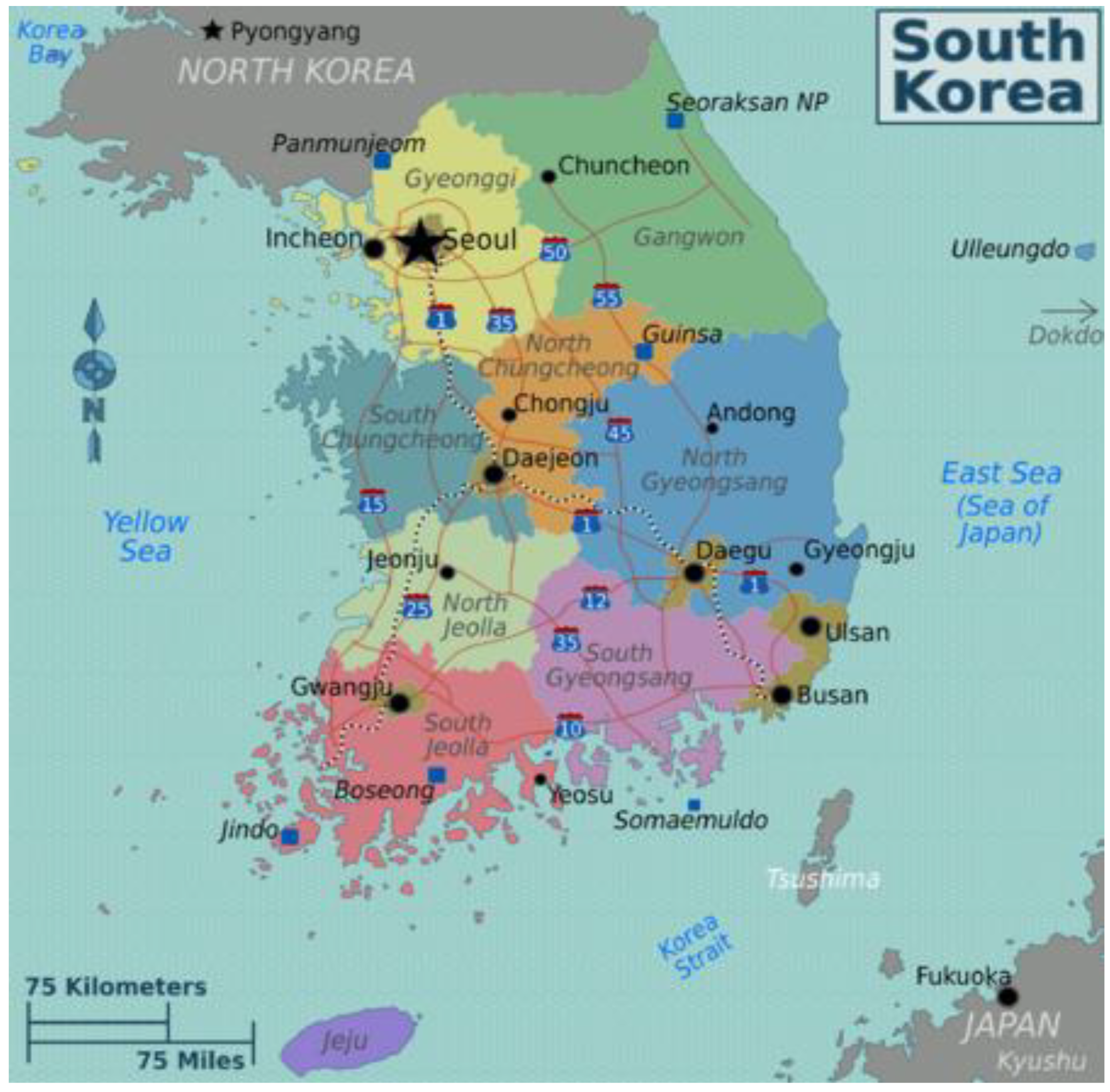
From the graph theory perspective, a node indicates a city or province in the container transport network. As seen in Figure 1, 16 nodes were identified. Except for Jejudo (geographically isolated from other regions, Jejudo has no railway lines; thus, we assume that there is only one cycle in Jejudo), each node has 56 arcs linking it to other nodes through roads and railways and one arc (the so-called “cycle”) denotes container transport within this region. As a result, there are 856 arcs (considering container incoming and outgoing, each node is connected to 14 other nodes through roads and railways, and each node has a cycle. Thus, we have (14 × 2 × 2 + 1) × 15 + 1 = 856 arcs in total) in total. However, for simplicity, we excluded arcs with volumes below a certain level in this case study.

3. Results

3.1. Parameter Estimation

To calculate the TNCI, we first consider the current cargo flow by railway. The freeware NodeXLGraph (https://nodexl.codeplex.com/) is used in this paper to represent the transport network as a graph. An arc will be removed if the number of containers transported by this arc is below 12, because regular service is defined as handling more than one container per month. With the help of the maximum standardization method, values on arcs, divided by the maximum value among all of the arcs, will lie between zero and one to reflect the number of containers handled between two different regions (Appendix A). As demonstrated in Figure 2, the size of each node is proportional to the total number of incoming and outgoing containers in this region. The width and direction of an arc reflect the number of containers handled from origin to destination.

Second, the current cargo flow by road can be analyzed in a similar way. However, in a graph representing the road container transport network, an arc with a cargo handling capacity below 10,000 TEU per month is removed. In general, Korean logistics companies provide more than 10,000 TEU line schedules per month between regions. In other words, when the cargo-handling capacity is below 10,000 TEU per month (Jejudo is not connected to other regions via roads or railways and it has a cycle of 72,047 TEU; it is thus not considered in the TNCI calculation because of its unique geographical location.), it is considered a non-regular service. The network is displayed in Figure 3. After comparing Figure 2 and Figure 3, it can be clearly seen that the arc distribution in the road network is thicker and more balanced than that in the railway network (Appendix B). This is because the road network has better accessibility, reachability, and capacity in South Korea, and thus it is more frequently utilized.

Third, with respect to capacity, calculations of road and railway capacity are quite challenging in civil engineering, because there are too many variables influencing the road and railway conditions [27]. Although some indicators, such as road or railway length, lane number, and type (express or non-express), can reflect road or railway capacity, it is hard to synthesize these data to obtain a comprehensive capacity indicator. To address this problem, the concept of source and sink in the graph theory is applied [6] (p. 173), [28]. In a directed graph, (a directed graph is a finite set of nodes, some of which are connected by arrows. In graph theory, a flow network, which is also known as a transportation network, is a directed graph where each edge has a capacity, and each edge receives flow. The amount of flow cannot exceed its capacity (https://en.wikipedia.org/wiki/Flow_network, a source is a node such that the arrows touching the node point away from the node, while a sink is a node such that all of the arrows touching the node point into the node. Likewise, in a transport network, a source generates flow, while a sink receives flow. Moreover, the flow in the network must arrive at the destination. Otherwise, the network will become jammed by overloading. When using containers for export, they are generally transported to ports via roads, railways, or inland waterways, and then they are transported to their destination ports by maritime transport. Meanwhile, when using containers for import, containers arriving at ports by maritime transport will be delivered all over the country by inland transport. In this sense, a port acts as both a source and a sink in container transport networks.

In the case of South Korea, we consider the Busan, Gwangyang, and Incheon ports, because these ports accounted for roughly 96% of the total container port throughput in 2010 (see

Table 2. Container throughput of main ports in South Korea in 2010 (1000 TEU).

	2007	2008	2009	2010	2011	2012	2013	2014
Busan	13,261	13,453	11,980	14,194	16,185	17,046	17,686	18,683
Gwangyang	1723	1810	1810	2073	2073	2154	2285	2338
Incheon	1664	1703	1578	1903	1998	1982	2161	2335
Others	699	757	697	783	856	890	905	938
% Top 3	96	96	96	96	96	96	96	96

Notes: Other includes the Pyeongtak and Ulsan ports. % Top 3 = 100×he container throughput of Busan, Gwangyang, and Incheon/Total container throughput of all the international trade ports in South Korea. Sources: Port authorities, The National Logistics Center, and Statistics Korea.

). In reality, the port capacity is usually calculated based on the container volume handled per year at the port.

Table 3. Capacity of the Busan, Gwangyang, and Incheon ports in 2010 (1000 TEU).

	Capacity	Number of Terminal
Busan	13,865	9
Gwangyang	4600	4
Incheon	1120	6
Total	19,585	19

Notes: The Busan container port has nine terminals (e.g., Jasungdae, Shinsundae, Gamman, Shin Gamman, Uam, Pusan New Port International Terminal, Pusan New Port Terminal, Hanjin New Port Terminal, and Hyundai Pusan New-port Terminal), the Gwangyang port has four sub-terminals, and the Incheon port has six sub-terminals, respectively. Regarding the Gwangyang port, container and bulk cargo are separated when calculating the transport network connectivity index (TNCI). Sources: Port authorities, The National Logistics Center, and Statistics Korea.

shows the capacity information provided by port authorities. From Table 3, capacities were 13,865,000 TEU, 4,600,000 TEU, and 1,120,000 TEU for the Busan, Gwangyang, and Incheon ports in 2010, respectively.

3.2. Calculation of the Connectivity Index

After estimating the required parameters, we move on to calculate the connectivity of the container transport networks in South Korea. As previously discussed, the Busan, Gwangyang, and Incheon ports can be seen as both sinks and sources. The TNCI can be calculated for each port to reflect its container transport network connectivity.

Table 4. Container throughput of the main ports based on graph theory (1000 TEU).

	Gwangyang	Incheon	Busan
Incoming	386	1123	7886
Outgoing	490	2284	3737
Cycle	1420	1785	2513
Total	2296	5192	14,136

Notes: Cycle indicates the transshipment of containers within or near a port. Total indicates the calculated container throughput. Sources: Port authorities, The National Logistics Center, and Statistics Korea.

reports the calculated incoming, outgoing, and cycle containers based on graph theory. As reported in Table 4, the container throughputs were 2,296,000 TEU, 5,192,000 TEU, and 14,136,000 TEU for the Gwangyang, Incheon, and Busan ports, respectively. To facilitate the daily operation of a port by giving users the information, notifications, and analysis that they need, port management information systems (PMISs) have been widely used around the world. As seen in

Table 5. Summary of container throughput of the main ports (1000 TEU). PMIS: port management information systems.

	Gwangyang	Incheon	Busan
Graph theory (GT) based	2296	5192	14,136
PMIS based	2088	1902	14,113
Capacity (C)	4600	1120	13,865
C-GT	2304	−4072	−271
C-PMIS	2512	−782	−248

Sources: Authors.

, the container throughputs based on the PMIS were 2,088,000 TEU, 1,902,000 TEU, and 14,113,000 TEU for the Gwangyang, Incheon, and Busan ports, respectively. The capacity of each port provided by port authorities is also given in Table 5. Then, the container throughput differences between the graph theory approach and the PMIS approach are larger in the cases of the Gwangyang and Incheon ports. A possible explanation lies in the type of cargo that is handled at each port. For example, the large percentage of dry bulk that is handled at the Gwangyang and the Incheon ports has to be transformed into TEU units for comparison, which could magnify the cargo flow.

Using Formula (7), we obtain the needed TNCIs and report them in

Table 6. Connectivity of container transportation networks in South Korea.

	Gwangyang	Incheon	Busan
${TNCI}_{GT}$	4,686,034	−7,626,677	−509,331
Standardized ${TNCI}_{GT}$	0.614426694	−1	−0.066782825
${TNCI}_{PMIS}$	5,078,824	−1,465,841	−464,534
Standardized ${TNCI}_{PMIS}$	1	−0.288618363	−0.091464971

Notes: Standardized $TNCI$ is obtained using the maximum standardization method. That is, the calculated $TNCI$ is divided by the absolute maximum. Sources: Authors.

. As revealed by the standardized TNCIs, in both cases, the Gwangyang port has the best connectivity, followed by the Busan port, and then the Incheon port. Specifically, the Busan and Incheon ports are found to have negative connectivity, indicating that their capacities are lower than the actual container flows. That is, congestions and delays are more likely to occur at these two ports. Therefore, it seems appropriate to expand the capacities of the Busan and Incheon ports. Due to different approaches for container flow calculations, the largest difference between TNCI based on graph theory and TNCI based on PMISs exists at the Incheon port. This suggests that a certain number of containers do not leave the network, but rather remain in the Incheon region, which in turn may cause congestion. Regarding the Gwangyang port, its positive connectivity reflects a higher capacity than the actual container flow. In fact, in the Korean logistics industry, there is a consensus that the Gwangyang port is too large. Thus, determining how to expand its hinterland and attract container flows is a logistical imperative.

4. Discussion

The calculated TNCIs provide valuable insights and guidance for policymakers. As suggested by Goldratt, the concept of a bottleneck, referring to a physical point or conceptual process that can decrease the efficiency of the whole system, is a suitable description of the container transport network in South Korea [29]. Inspired by the bottleneck concept, nodes with negative connectivity are identified as bottlenecks. In the case study, the Busan and Incheon ports act as bottlenecks in the whole container transport network. Moreover, most containers are transported via roads in South Korea, and relatively low efficiency can be observed in road transport, which negatively affects the connectivity of container transport networks and influences the local economy in a non-sustainable manner.

Accordingly, specific strategies can be suggested for port development. For example, in the case of the Incheon port, a strategy for port capacity expansion seems to be appropriate, because the capacity is much lower than the actual container flow. Although the Busan port has a negative connectivity, the small difference between the capacity and the actual container flow suggests that a strategy for improvement in operational efficiency might be most suitable, such as the enhancement of cooperation among terminal operators or an emphasis on port employee training and qualifications. Regarding the Gwangyang port, a strategy for port hinterland expansion is needed to attract more container flows. In the meantime, port users can also benefit from the TNCIs that help them identify ports that have better inland transport connectivity. This in turn increases port users’ satisfaction and enhances port reputation as well as port competitiveness. In addition, container transport relies heavily on road transport in South Korea, placing a considerable burden on road transport. Meanwhile, the supply of railway container transport services is relatively low in South Korea. As a result, how to increase available railway container transport services is particularly important for policymakers. As an alternative transport mode, an increase in the demand for railway container transport would be helpful to reduce road container flows, and then could improve the overall connectivity of container transport networks.

5. Conclusions

Container transport has played an ever-important role in promoting South Korea’s sustainable economy, which requires a better connectivity of container transport networks. For this purpose, we develop an index to assess container transport network connectivity from the multi-modal transport perspective. The calculated connectivity index not only provides insight into the assessment of sustainable port competitiveness, it also helps policymakers identify bottlenecks in multi-modal transport networks. Specifically, from the congestion perspective, a well-connected port usually indicates that the capacity is higher than the usage of links. The lower the difference, the higher the possibility of observing congestion in container transport networks. This potentially reduces port attractiveness and moves shipping lines to call at other ports. In this sense, the connectivity index can be used as a criterion for shipping lines’ port selection. On the other hand, the probability of congestion becomes higher when the cargoes that are handled in a port are higher than the capacity, which usually indicates that the links are over-utilized. This also reflects that the container transport network is not well-connected because of insufficient capacity, which in turn motivates capacity investment. In this regard, the developed connectivity index can also be used as a criterion for policymakers’ investment decisions.

Using container transport in South Korea as a case study, some specific strategies are proposed to improve port operations. For the Incheon port, it is suggested that port capacity needs to be expanded to facilitate the increasing container flows, resulting in the lower possibility of observing congestions and delays. For the Busan port, more emphasis should be placed on improvements in operational efficiency by effectively cooperating with terminal operators and training port employees. For the Gwangyang port, the recommendation is to expand its hinterland and attract more container flows. At the same time, the bottleneck analysis also provides valuable insight and guidance for port users who would benefit from identifying ports with superior container transport network connectivity. In addition, expanding the supply of railway container transport services in South Korea could reduce its heavy reliance on road transport.

Nevertheless, some potential limitations still exist in the current paper. For example, we only consider connectivity for a single year, which may not enable us to explore the evolution of connectivity in container transport networks over time or model the future connectivity. Another limitation is the potential underestimation of the road container cargo flow when using the maximum weight of a container cargo trailer to convert the tonnage data. However, these limitations do present a new perspective and avenue for our future research.

References

- Review of Maritime Transport; United Nations Conference on Trade and Development: New York, NY, USA; Geneva, Switzerland, 2017; Available online: http://unctad.org/en/PublicationsLibrary/rmt2017_en.pdf (accessed on 1 October 2018).
- Maloni, M.J.; Gligor, D.M.; Lagoudis, I.N. Linking ocean container carrier capabilities to shipper–carrier relationships: A case study. Marit. Policy Manag. 2016, 43, 959–975. [Google Scholar] [CrossRef]
- De Langen, P.W.; Haezendonck, E. Ports as clusters of economic activity. In Maritime Economics; Wiley-Blackwell: Hoboken, NJ, USA, 2012; pp. 638–655. [Google Scholar]
- Shi, W.; Li, K.X. Themes and tools of maritime transport research during 2000–2014. Marit. Policy Manag. 2017, 44, 151–169. [Google Scholar] [CrossRef]
- Ferrari, C.; Parola, F.; Gattorna, E. Measuring the quality of port hinterland accessibility: The Ligurian case. Transp. Policy 2011, 18, 382–391. [Google Scholar] [CrossRef]
- Janic, M.; Regglani, A.; Nijkamp, P. Sustainability of the European freight transport system: Evaluation of innovation bundling networks. Transp. Plan. Technol. 1999, 23, 129–156. [Google Scholar] [CrossRef]
- Di Vaio, A.; Varriale, L. Management innovation for environmental sustainability in seaports: Managerial accounting instruments and training for competitive green ports beyond the regulations. Sustainability 2018, 10, 783. [Google Scholar] [CrossRef]
- Diestel, R. Graph Theory, 4th ed.; Graduate Texts in Mathematics; Springer: Berlin/Heidelberg, Germany, 2018; p. 173. [Google Scholar]
- Arvis, J.F.; Shepherd, B. The Air Connectivity Index: Measuring Integration in the Global Air Transport Network; Policy Research Working Paper; The World Bank: Washington, DC, USA, 2011; p. 5722. [Google Scholar]
- Hoffman, J.; Wilmsmeier, G. Liner shipping connectivity and port infrastructure as determinants of freight rates in the Caribbean. Marit. Econ. Logist. 2008, 10, 130–151. [Google Scholar]
- Gwartney, J.; Lawson, R.; Hall, J. 2014 Economic Freedom Dataset. Economic Freedom of the World: 2014 Annual Report; Fraser Institute: Vancouver, BC, Canada, 2014. [Google Scholar]
- Welch, T.F. Equity in transport: The distribution of transit access and connectivity among affordable housing units. Transp. Policy 2013, 30, 283–293. [Google Scholar] [CrossRef]
- Kaplan, S.; Popoks, D.; Prato, C.C.; Ceder, A. Using connectivity for measuring equity in transit provision. J. Transp. Geogr. 2014, 37, 82–92. [Google Scholar] [CrossRef]
- Lundberg, B.; Weber, J. Non-motorized transport and university populations: An analysis of connectivity and network perceptions. J. Transp. Geogr. 2014, 39, 165–178. [Google Scholar] [CrossRef]
- Antonson, H.; Gustafsson, M.; Angelstam, P. Cultural heritage connectivity. A tool for EIA in transportation infrastructure planning. Transp. Res. Part D 2010, 15, 463–472. [Google Scholar] [CrossRef]
- Derudder, B.; Liu, X.; Kunaka, C.; Roberts, M. The connectivity of South Asian cities in infrastructure networks. J. Maps 2014, 10, 47–52. [Google Scholar] [CrossRef] [Green Version]
- Lam, J.S.L.; Yap, W.Y. Dynamics of liner shipping network and port connectivity in supply chain systems: Analysis on East Asia. J. Transp. Geogr. 2011, 19, 1272–1281. [Google Scholar] [CrossRef]
- Jiang, J.; Lee, L.H.; Chew, E.P.; Gan, C.C. Port connectivity study: An analysis framework from a global container liner shipping network perspective. Transp. Rese. Part E Logist. Transp. Rev. 2015, 73, 47–64. [Google Scholar] [CrossRef]
- Yang, D.; Wang, S. Analysis of the development potential of bulk shipping network on the Yangtze River. Marit. Policy Manag. 2017, 44, 512–523. [Google Scholar] [CrossRef]
- Tovar, B.; Hernández, R.; Rodríguez-Déniz, H. Container port competitiveness and connectivity: The Canary Islands main ports case. Transp. Policy 2015, 38, 40–51. [Google Scholar] [CrossRef]
- Du, Y.; Meng, Q.; Wang, S. Mathematically calculating the transit time of cargo through a liner shipping network with various trans-shipment policies. Marit. Policy Manag. 2017, 44, 248–270. [Google Scholar] [CrossRef]
- Alstadt, B.; Weisbrod, G.; Cutler, D. The relationship of transportation access and connectivity to local economic outcomes: A statistical analysis. J. Transp. Res. Board 2012, 2297, 154–162. [Google Scholar] [CrossRef]
- Beaudoin, J.; Farzin, Y.H.; Lawell, C.Y.C.L. Public transit investment and sustainable transportation: A review of studies of transit’s impact on traffic congestion and air quality. Res. Transp. Econ. 2015, 52, 15–22. [Google Scholar] [CrossRef]
- Chang, G.; Xiang, H. The Relationship between Congestion Levels and Accidents; Maryland State Highway Administration: Baltimore, MD, USA, 2003.
- Kim, C.B. Estimating and forecasting the trading volumes of airway transport. Air Transp. J. 2007, 10, 78–99. [Google Scholar]
- Peng, W.Y.; Chu, C.W. A comparison of univariate methods for forecasting container throughput volumes. Math. Comput. Model. 2009, 50, 1045–1057. [Google Scholar] [CrossRef]
- Garber, N.; Hoel, L. Traffic and Highway Engineering; Cengage Learning: Boston, MA, USA, 2014. [Google Scholar]
- Gibbons, A. Algorithmic Graph Theory; Cambridge University Press: Cambridge, UK, 1985. [Google Scholar]
- Goldratt, E.M. Theory of Constraints; North River: Croton-on-Hudson, NY, USA, 1990. [Google Scholar]
Figure 1.
Administrative divisions of South Korea.
Figure 2.
The current railway cargo flow. Sources: Authors.
Figure 3.
The current cargo road cargo flow. Sources: Authors.