Optimal Pricing and Service for the Peak-Period Bus Commuting Inefficiency of Boarding Queuing Congestion


Abstract
1. Introduction
2. Literature Review
3. Peak Period Equilibrium Bus Boarding Model
3.1. Problem Description
3.2. Symbols
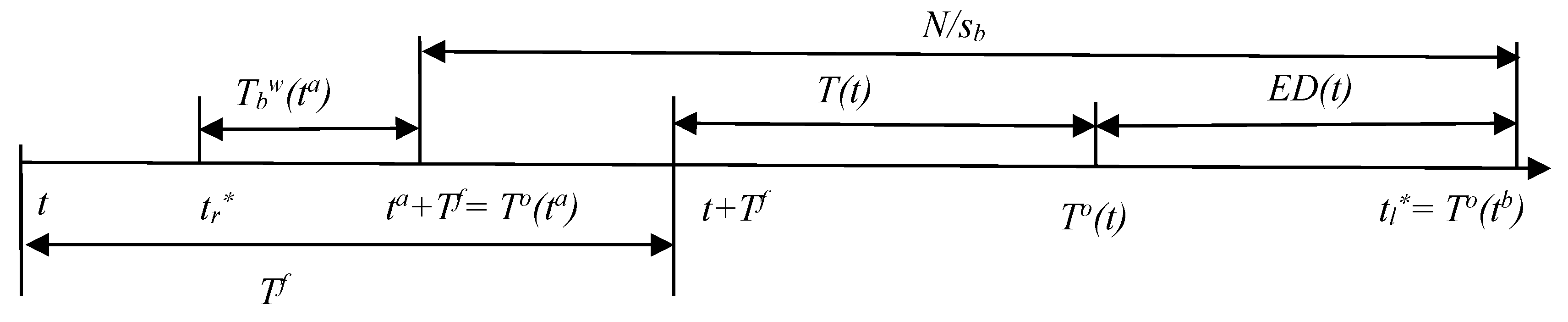
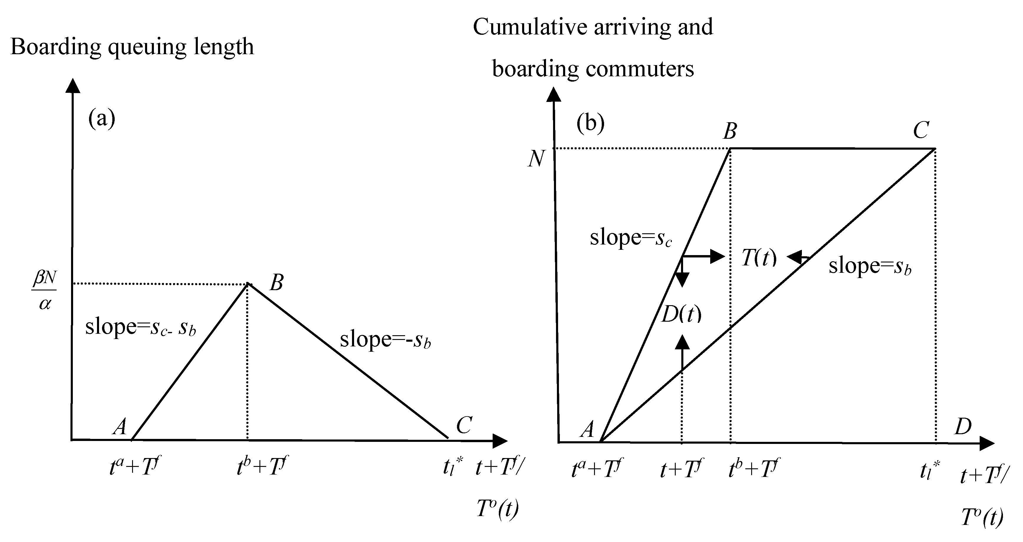
3.3. The Model
4. Analysis
4.1. No-Toll Equilibrium Analysis
4.2. Social Optimal Equilibrium Analysis
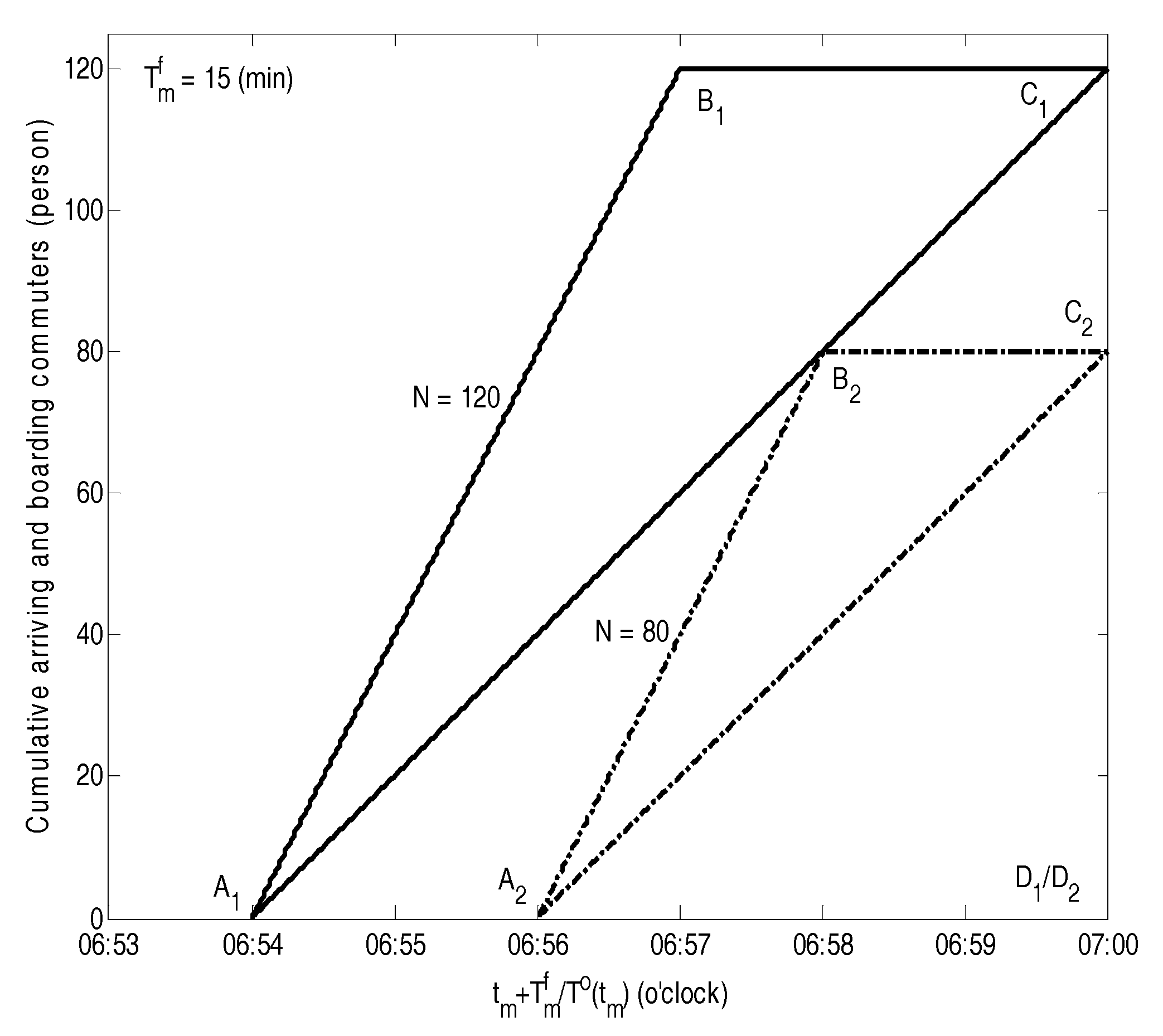
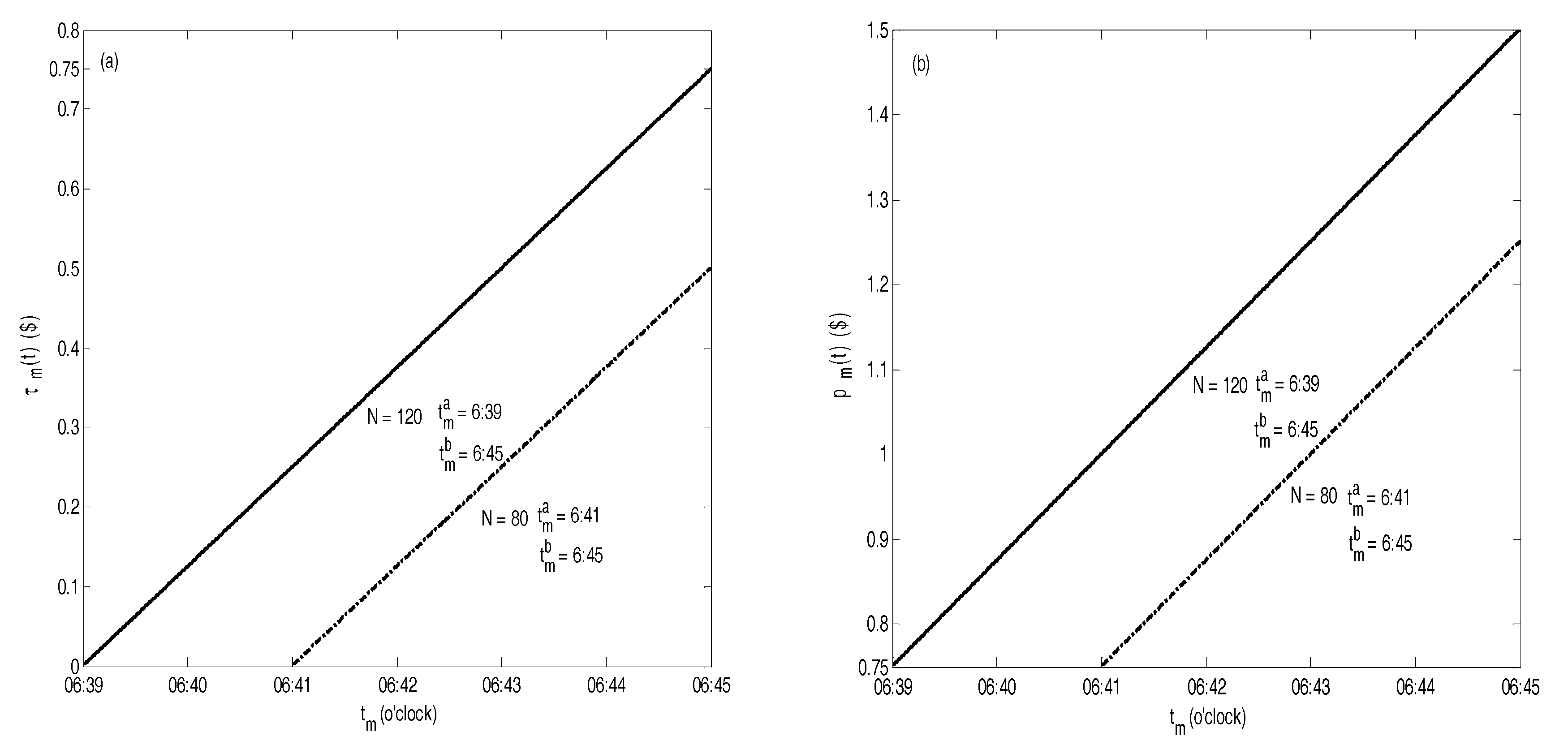
5. Numerical Analysis
6. Conclusions
Author Contributions
Funding
Acknowledgments
Conflicts of Interest
Appendix A. Derivation of the Optimal Bus Departure Interval during the Peak Period
References
- Vickrey, W.S. Congestion theory and transport investment. Am. Econ. Rev. 1969, 59, 251–260. [Google Scholar]
- Arnott, R.; de Palma, A.; Lindsey, R. Schedule delay and departure time decisions with heterogeneous communeters. Transp. Res. Rec. 1988, 1197, 56–67. [Google Scholar]
- Arnott, R.; de Palma, A.; Lindsey, R. Economics of a bottleneck. J. Urban Econ. 1990, 27, 111–130. [Google Scholar] [CrossRef]
- Arnott, R.; de Palma, A.; Lindsey, R. Route choice with heterogeneous drivers and group-specific congestion costs. Reg. Sci. Urban Econ. 1992, 22, 71–102. [Google Scholar] [CrossRef]
- Arnott, R.; de Palma, A.; Lindsey, R. The welfare effects of congestion tolls with heterogeneous commuters. J. Transp. Econ. Policy 1994, 28, 139–161. [Google Scholar]
- Arnott, R.; DePalma, E. The corridor problem: Preliminary results on the no-toll equilibrium. Transp. Res. Part B 2001, 45, 743–768. [Google Scholar] [CrossRef]
- Lindsey, R. Existence, uniqueness, and trip cost function properties of user equilibrium in the botteneck model with multiple user classes. Transp. Sci. 2004, 38, 293–314. [Google Scholar] [CrossRef]
- Van den Berg, V.; Verhoef, E.T. Congestion tolling in the bottleneck model with heterogeneous values of time. Transp. Res. Part B 2011, 45, 60–78. [Google Scholar] [CrossRef]
- Li, Z.C.; Lam, W.H.K.; Wong, S.C. Step tolling in an activity-based bottleneck model. Transp. Res. Part B 2017, 101, 306–334. [Google Scholar] [CrossRef]
- Guo, R.Y.; Yang, H.; Huang, H.J.; Li, X.W. Day-to-day departure time choice under bounded rationality in the bottleneck model. Transp. Res. Procedia 2017, 23, 551–570. [Google Scholar] [CrossRef]
- Knockaert, J.; Verhoef, E.T.; Rouwendal, J. Bottleneck congestion: Differentiating the coarse charge. Transp. Res. Part B 2016, 83, 59–73. [Google Scholar] [CrossRef]
- Khan, Z.; Amin, S. Bottleneck model with heterogeneous information. Transp. Res. Part B 2018, 112, 157–190. [Google Scholar] [CrossRef]
- de Palma, A.; Arnott, R. The temporal use of a telephone line. Inf. Econ. Policy 1990, 4, 155–174. [Google Scholar] [CrossRef]
- Tian, Q.; Huang, H.J.; Yang, H.; Gao, Z.Y. Efficiency and equity of ramp control and capacity allocation mechanisms in a freeway corridor. Transp. Res. Part C 2012, 20, 126–143. [Google Scholar] [CrossRef]
- Chen, D.; Zhang, N.; Liu, J. Effect of road traffic congestion on aviation passenger’s flight choice. J. Transp. Syst. Eng. Inf. Technol. 2013, 13, 96–102. [Google Scholar] [CrossRef]
- Takayama, K.; Kuwahara, M. Bottleneck congestion and residential location of heterogeneous commuters. J. Urban Econ. 2017, 100, 65–79. [Google Scholar] [CrossRef]
- Mohring, H. Optimization and scale economies in urban bus transportation. Am. Econ. Rev. 1972, 62, 591–604. [Google Scholar]
- Jansson, J.O. A simple bus line model for optimisation of service frequency and bus size. J. Transp. Econ. Policy 1980, 14, 53–80. [Google Scholar]
- Sumi, T.; Matsumoto, Y.; Miyaki, Y. Departure time and route choice of commuters on mass transit systems. Transp. Res. Part B 1990, 24, 247–262. [Google Scholar] [CrossRef]
- Alfa, A.S.; Chen, M. Temporal distribution of public transport demand during the peak period. Eur. J. Oper. Res. 1995, 83, 137–153. [Google Scholar] [CrossRef]
- Tian, Q.; Huang, H.J.; Yang, H. Equilibrium properties of the morning peak-period commuting in a many-to-one mass transit system. Transp. Res. Part B 2007, 41, 616–631. [Google Scholar] [CrossRef]
- Kraus, M.; Yoshida, Y. The commter’s time-of-use decision and optimal pricing and service in urban mass transit. J. Urban Econ. 2002, 51, 170–195. [Google Scholar] [CrossRef]
- Kraus, M. A new look at the two-mode problem. J. Urban Econ. 2003, 54, 511–530. [Google Scholar] [CrossRef]
- Kraus, M. Road pricing with optimal mass transit. J. Urban Econ. 2012, 72, 81–86. [Google Scholar] [CrossRef]
- Ruiz, M.; Segui-Pons, J.M.; Mateu-LLadó, J. Improving Bus Service Levels and social equity through bus frequency modeling. J. Transp. Geogr. 2017, 58, 220–233. [Google Scholar] [CrossRef]
- AlKheder, S.; AlRukaibi, F.; Zaqzouq, A. Optimal bus frequency for Kuwait public transportation company: A cost view. Sustain. Cities Soc. 2018, 41, 312–319. [Google Scholar] [CrossRef]
- Wang, D.Z.W.; Nayan, A.; Szeto, W.Y. Optimal bus service design with limited stop services in a travel corridor. Transp. Res. Part A 2018, 111, 70–86. [Google Scholar] [CrossRef]
- Börjesson, M.; Fung, C.M.; Proost, S. Optimal prices and frequencies for buses in Stockholm. Econ. Transp. 2017, 9, 20–36. [Google Scholar] [CrossRef]
- Sun, L.; Tirachini, A.; Axhausen, K.W.; Erath, A.; Lee, D.H. Models of bus boarding and alighting dynamics. Transp. Res. Part A 2014, 69, 447–460. [Google Scholar] [CrossRef]
- Tirachini, A.; Hensher, D.A. Bus congestion, optimal infrastructure investment and the choice of a fare collection system in dedicated bus corridors. Transp. Res. Part B 2011, 45, 828–844. [Google Scholar] [CrossRef]
- Guenthner, R.P.; Hamat, K. Transit dwell time under complex fare structure. J. Transp. Eng. ASCE 1998, 114, 279–367. [Google Scholar] [CrossRef]
- Levine, J.C.; Torng, G.W. Dwell-time effects of low-floor bus design. J. Transp. Eng. ASCE 1994, 120, 914–929. [Google Scholar] [CrossRef]
- Dorbritz, R.; Lüthi, M.; Weidmann, U.; Nash, A. Effects of onboard ticket sales on public transport reliability. Transp. Res. Rec. 2009, 2110, 112–119. [Google Scholar] [CrossRef]
- Fernández, R.; Zegers, P.; Weber, G.; Tyler, N. Influence of platform height, door width, and fare collection on bus dwell time. Transp. Res. Rec. 2010, 2143, 59–66. [Google Scholar] [CrossRef]
- Tirachini, A. Bus dwell time: The effect of different fare collection systems, bus floor level and age of passengers. Transp. A Transp. Sci. 2013, 9, 28–49. [Google Scholar] [CrossRef]
- Fletcher, G.; El-Geneidy, A. The effects of fare payment types and crowding on dwell time: A fine-grained analysis. Transp. Res. Rec. 2013, 2351, 124–132. [Google Scholar] [CrossRef]
- D’Souza, C.; Paquet, V.; Lenker, J.A.; Steinfeld, E. Effects of transit bus interior configuration on performance of wheeled mobility users during simulated boarding and disembarking. Appl. Ergon. 2017, 62, 94–106. [Google Scholar] [CrossRef] [PubMed]
- Wu, W.T.; Liu, R.H.; Jin, W.Z. Modelling bus bunching and holding control with vehicle overtaking and distributed passenger boarding behaviour. Transp. Res. Part B 2017, 104, 175–197. [Google Scholar] [CrossRef]
- Ji, Y.J.; Gao, L.P.; Chen, D.D.; Ma, X.W.; Zhang, R.C. How does a static measure influence passengers’ boarding behaviors and bus dwell time? Simulated evidence from Nanjing bus stations. Transp. Res. Part A 2018, 110, 13–25. [Google Scholar] [CrossRef]
- Small, K.A. The scheduling of consumer activities: Work trips. Am. Econ. Rev. 1982, 72, 467–479. [Google Scholar]


| Selected Reference | Methodology | Characteristics |
|---|---|---|
| Vickrey [1] | First bottleneck model | Equilibrium queuing patterns at a single bottleneck on freeways to a work place during the morning peak period |
| Arnott et al. [3] | The extended bottleneck model | Queue delay at the bottleneck can be eliminated by time-varying pricing |
| Mohring [17] | The bus line model: the basic model of optimal pricing and service in urban mass transit | The square root principle: the optimal bus frequency is proportional to the square root of the number of commuters |
| Jansson [18] | A model extended the square root principle | Service frequency was simultaneously optimized with bus size |
| Tian et al. [21] | An equilibrium model of peak-period commuting for a mass transit line | Queuing time at station is zero for simplicity and the general properties of the equilibrium departure time distribution of commuters |
| Kraus and Yoshida [22] | The rail line model: queuing time at a transit stop is treated analogously to queuing time at a bottleneck | Economic analyses of the commuters’ time-of-use decision, the optimal pricing, and the service in urban mass transit and under the optimal pattern of arrivals decentralized with an appropriate run-dependent fare, no queuing actually occurs |
| Sun et al. [29] | The first use of smart card data | Bus passenger boarding behavior and its impact on bus dwell time |
| This paper | The equilibrium bus boarding model: queuing time at the bus station is treated analogously to queuing time at a bottleneck | Dynamic boarding queuing congestion toll can indicate the social optimal equilibrium and the optimal bus departure interval during the peak period, which does not conform to the square root principle |
| Symbol | Meaning/Description |
|---|---|
| Number of the identical commuters of the bus | |
| Commuter’s departure time | |
| The earliest boarding commuter’s departure time | |
| The last boarding commuter’s departure time | |
| Travel time of the commuter from the origin to the bus station, which is assumed to be the same for all commuters | |
| The time when the bus arrives at the bus station | |
| The time when the bus leaves from the bus station | |
| The time that the arrival bus waits for the earliest boarding commuter at the bus station | |
| Boarding capacity of the bus | |
| Boarding queuing time of the commuter departing at time t at the bus station | |
| Boarding time of the commuter departing at time t | |
| Time that elapses from the boarding time of the commuter to the time that the commuter chooses the seat or the standing position in the bus, which is ignored | |
| Boarding queuing time of the commuter departing at time t | |
| Early boarding delay of the commuter departing at time t | |
| Travel cost of the commuter departing at time t | |
| Unit travel time cost | |
| Unit early boarding delay cost | |
| The static fare | |
| Equilibrium travel cost | |
| Commuter departure rate | |
| Boarding queuing length at different time | |
| Total boarding queuing time of all commuters on the bus | |
| Total early boarding delay cost of all commuters on the bus | |
| Total equilibrium travel cost of all commuters on the bus | |
| Dynamic boarding queuing congestion toll | |
| Total dynamic boarding queuing congestion toll for all commuters on the bus | |
| Dynamic fare | |
| the subscript | Morning peak-period bus commuting |
| min | Minute |
| , | Number of commuters on the preceding bus and the following bus , respectively |
| , | Boarding capacity of the preceding bus and the following bus , respectively |
| , | Departure time of the preceding bus and the following bus at the last bus station, respectively |
| , | The time the preceding bus and the following bus spend on arriving at the bus station from the last bus station, respectively |
| The earliest boarding commuter’s departure time of the following bus | |
| The last boarding commuter’s departure time of the preceding bus | |
| Bus departure interval, | |
| The time the following bus arrives at the bus station | |
| The time the preceding bus leaves the bus station |
© 2018 by the authors. Licensee MDPI, Basel, Switzerland. This article is an open access article distributed under the terms and conditions of the Creative Commons Attribution (CC BY) license (http://creativecommons.org/licenses/by/4.0/).
Share and Cite
Zeng, Y.-Z.; Ran, B.; Zhang, N.; Yang, X.; Shen, J.-J.; Deng, S.-J. Optimal Pricing and Service for the Peak-Period Bus Commuting Inefficiency of Boarding Queuing Congestion. Sustainability 2018, 10, 3497. https://doi.org/10.3390/su10103497
Zeng Y-Z, Ran B, Zhang N, Yang X, Shen J-J, Deng S-J. Optimal Pricing and Service for the Peak-Period Bus Commuting Inefficiency of Boarding Queuing Congestion. Sustainability. 2018; 10(10):3497. https://doi.org/10.3390/su10103497
Chicago/Turabian StyleZeng, You-Zhi, Bin Ran, Ning Zhang, Xiaobao Yang, Jia-Jun Shen, and She-Jun Deng. 2018. "Optimal Pricing and Service for the Peak-Period Bus Commuting Inefficiency of Boarding Queuing Congestion" Sustainability 10, no. 10: 3497. https://doi.org/10.3390/su10103497
APA StyleZeng, Y.-Z., Ran, B., Zhang, N., Yang, X., Shen, J.-J., & Deng, S.-J. (2018). Optimal Pricing and Service for the Peak-Period Bus Commuting Inefficiency of Boarding Queuing Congestion. Sustainability, 10(10), 3497. https://doi.org/10.3390/su10103497