Using Soil Survey Database to Assess Soil Quality in the Heterogeneous Taihang Mountains, North China


1
Key Laboratory of Ecosystem Network Observation and Modeling, Institute of Geographic Sciences and Natural Resources Research, Chinese Academy of Sciences, Beijing 100101, China
2
College of Resources and Environment, University of Chinese Academy of Sciences, Beijing 100049, China
*
Author to whom correspondence should be addressed.
Sustainability 2018, 10(10), 3443; https://doi.org/10.3390/su10103443
Submission received: 21 August 2018
/
Revised: 14 September 2018
/
Accepted: 25 September 2018
/
Published: 27 September 2018
Abstract
:Soil quality evaluation is an effective pathway to understanding the status of soil function and ecosystem productivity. Numerous studies have been made in managed ecosystems and land cover to quantify its effects on soil quality. However, little is coincident regarding soil quality assessment methods and its compatibility in highly heterogeneous soil. This paper used the soil survey database of Taihang Mountains as a case study to: (i) Examine the feasibility of soil quality evaluation with two different indicator methods: Total data set (TDS) and minimum data set (MDS); and (ii) analyze the controlling factors of regional soil quality. Principal component analysis (PCA) and the entropy method were used to calculate soil quality index (SQI). SQI values assessed from the TDS and MDS methods were both significantly correlated with normalized difference vegetation index (p < 0.001), suggesting that both indices were effective to describe soil quality and reflect vegetation growth status. However, the TDS method represented a slightly more accurate assessment than MDS in terms of variance explanation. Boosted regression trees (BRT) models and path analysis showed that soil type and land cover were the most important controlling factors of soil quality, within which soil type had the greatest direct effect and land cover had the most indirect effect. Compared to MDS, TDS is a more sensitive method for assessing regional soil quality, especially in heterogeneous mountains. Soil type is the fundamental factor to determining soil quality. Vegetation and land cover indirectly modulate soil properties and soil quality.
1. Introduction
Soil quality has been a key issue in agrology, agronomy, and environmental science with the increasing awareness of its importance in soil management and ecosystem sustainability [1]. Numerous definitions of soil quality have been proposed since the 1990s [2,3,4,5], among which the most widely adopted one is the capacity of soil to sustain biological productivity, maintain soil function and environmental quality, and promote plant and animal health within ecosystem boundaries [6,7]. In other words, maintaining vegetation productivity without degrading environmental sustainability is the core of soil quality. Therefore, the quantification of soil quality is of great significance to understand soil nutrient conditions and identify problem areas before formulating targeted schemes for sustainable land use management [8].
Accurately and reliably evaluating soil quality is essential for a better understanding of soil function and making wise decisions in sustainable soil management and land use [9]. However, soil quality evaluation is still ongoing in the field of soil science. Although many methods have been developed, there is no universal method to determine soil quality [8,10]. Soil quality indices (SQIs) are commonly used methods so far and have been proven to be a successful tool of reflecting soil quality conditions [9,11]. A robust SQI should be: (i) Sensitive to soil management; (ii) sensitive to changes in soil function(s); and (iii) easily measurable [12]. SQI cannot be directly measured, but it is generally developed through score-based integration of selected physical, chemical, and biological soil properties into an index. This process commonly involves three steps: First, selecting a representative data set of soil properties in relation to a particular soil function, then normalizing these soil properties into unitless scores, and finally integrating the scores into an index [8,11,13,14]. Indicator selection is the most important step, because it can influence evaluation results from the beginning. However, there is no consistent methodology so far to select a universal data set to characterize soil quality across all regions and scales [15]. Therefore, many SQIs have been proposed, according to specific purposes. For example, nutrient elements related to crop yield are usually included in farmland quality evaluation [16], while mine soil quality assessment has to consider heavy metal concentration threshold [17]. In most of the previous studies [8,18,19], soil organic matter is regarded as a critical indicator for soil quality evaluation. Other soil properties such as nitrogen, phosphorous, potassium, soil texture, cation exchange capacity, bulk density, and potential of hydrogen (pH) value are also believed to have a considerable impact on soil quality. This has raised concerns about the selection of essential indicators for soil quality.
Most previous studies collected the data of soil properties from field sampling and laboratory measurements [10,20]. Soil quality evaluation based on the total data set (TDS) of soil properties includes more information and results in a more comprehensive and accurate outcome if data are accessible [8,9,21]. However, data acquisition requires too much analysis if the study sites are extended to regions, thereby becoming costly, labor-intensive, and time-consuming. Some techniques, such as pedotransfer functions [22], local farmer knowledge [23], and visible—near—infrared spectroscopy [24] are proposed to simplify and accelerate the procedure of acquiring data of soil properties. Soil quality evaluations with these techniques are often conducted at low spatial resolution. However, soil database, an essential component of soil quality evaluation [25], especially for large scales such as regional, national, or even global levels, is seldom used to evaluate soil quality. A minimum data set (MDS) is recommended to be the most suitable method to represent soil quality indicators, especially for large-scale evaluation. Previous studies have proven that the MDS method has the capacity to select key indicators which contained adequate information for soil quality assessment. Moreover, the MDS method can reduce the number of indicators so that the work of laboratory analysis would be lessened [8,9]. Nevertheless, compared to the MDS method, TDS is found more informative [9], and perhaps is more effective in large-scale soil quality evaluation. However, comparison of TDS and MDS in the quantification of soil quality is rarely evaluated regionally.
In addition, more studies are focused on defining and assessing soil quality more than on analyzing factors influencing soil quality. Furthermore, most of these limited factor analyzing studies only concerned fertilization management as the factor affecting soil organic matter or carbon content rather than soil quality [26,27,28]. However, other factors, such as soil parent material, land cover, topography, and climate also hold the key to soil quality, especially in mountainous areas with highly spatial heterogeneity. For example, soil type is associated with parent materials and thus a crucial factor affecting soil erosion and organic matter [29,30]. Soil loss and soil quality also vary with vegetation and/or land use and land cover [29,31]. In mountainous areas, elevation and slope are important topographic factors and research suggests that they both have a great effect on soil quality and erosion rates [29,32]. In addition, soil water availability shows significant effects on aggregate size distribution in semi-arid areas [33]. Unfortunately, it remains unclear how important these factors will be to soil quality, particularly in highly heterogeneous mountainous areas.
Located in the earth-rocky mountainous region of northern China, Taihang Mountains are the transition zone of Loess Plateau and North China Plain. They are highly heterogeneous due to dramatic changes in terrain, soil type, and vegetation [34,35]. Some studies have attempted to address small-scale soil quality in the Taihang Mountains. For example, Du [36] analyzed the influences of conservation tillage practices on soil quality in the piedmont plain of the Taihang Mountains. Liu [37] discussed the effect of land cover changes on soil chemical properties. Yang [38] investigated the spatial distribution of soil heavy metals in Taihang piedmont Plain. All these studies, usually based on catchment or county scale, focused on the present status of some soil properties and their changes with external forces. However, a holistic cognition of soil quality is still lacking in the Taihang Mountains. As such, the objectives of this study were to: (i) Propose suitable methods for soil quality evaluation of the Taihang Mountains using soil database; (ii) compare soil quality assessment based on TDS and MDS and then identify the appropriate indicator selection method for assessing soil quality; and (iii) explore the controlling factors of soil quality.
2. Materials and Methods
2.1. Study Area Description
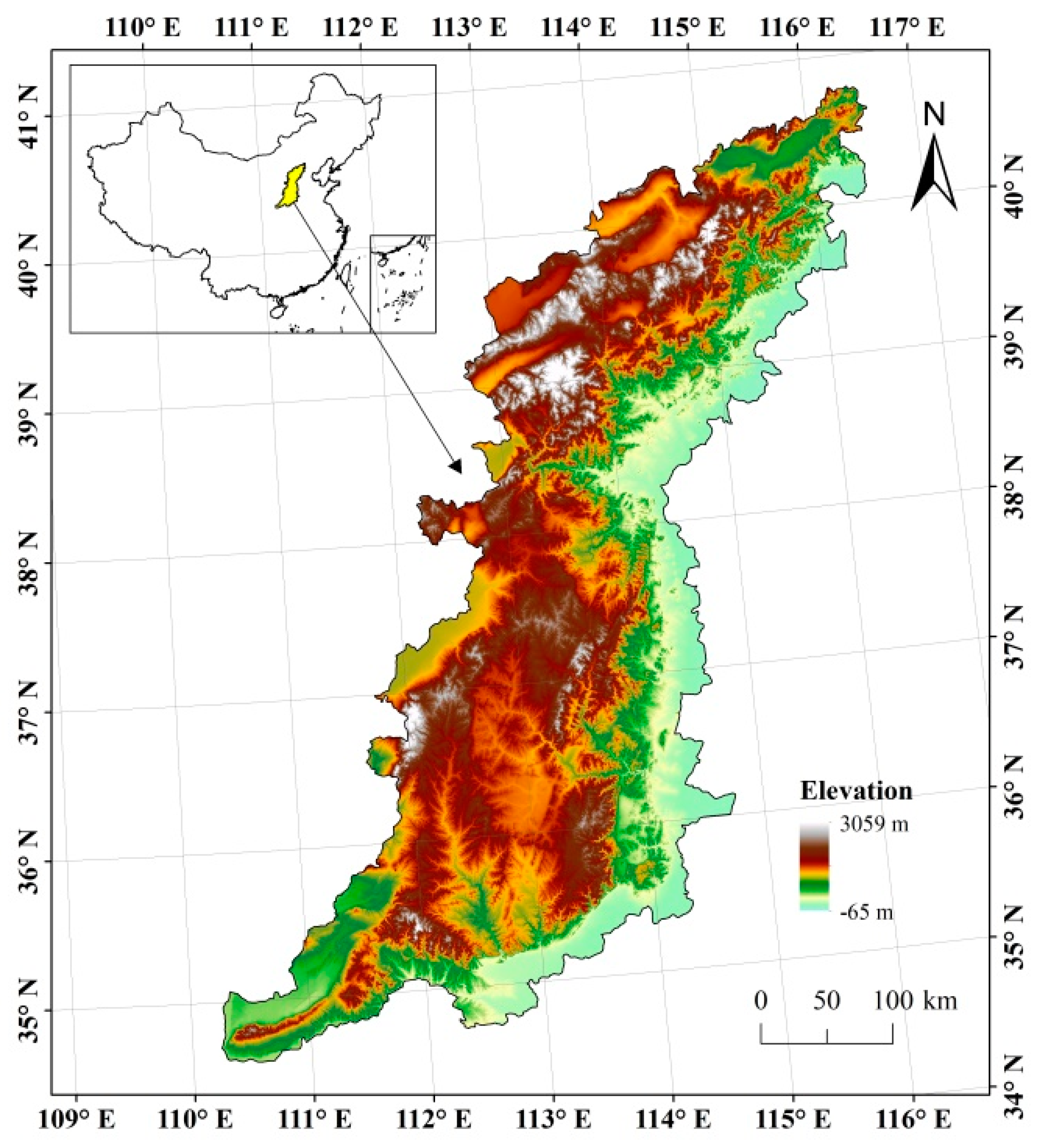
The Taihang Mountains (34°15′–41°09′ N, 110°14′–116°35′ E), stretching 400 km from north to south in northern China, cover an area of ca. 136,000 km2 (Figure 1). They are the transition zone between the North China Plain and Loess Plateau and the demarcation line of semihumid and semiarid climate from east to west, respectively. The study area has predominantly mountainous topography with an average elevation of 1000–1500 m, which decreases from the northwest to the southeast [34]. Climate belongs to a semihumid warm temperate continental monsoon type, characterized by distinct seasonal variation with an annual average temperature of 7.3–12.7 °C and annual average precipitation of 560 mm, of which 70–80% occurs between June and August. Due to terrain variation and temperature, precipitation gradients, highly heterogeneous soil, and vegetation types present in the study area, soils in the Taihang Mountains develop mainly from limestone in the northern and southern parts, but from gneiss in the middle region. The soil layers are thin, but with abundant gravel content. There are 28 categories of soil type, based on the Food and Agriculture Organization (FAO-90) soil classification system [34]. Vegetation patterns are significantly affected by topography, elevation, slope, and aspect, as well as the interactions between these environmental factors [35]. The Taihang Mountains represent the convergence zone of the southern and northern floras of the East Asian continent, with species turnover from deciduous broadleaf to coniferous species, along with an increase in elevation, and from the south to north. Vegetation is composed of temperate forests dominant by Quercus spp., Betula platyphylla, Larix principis-rupprechtii. There are obvious vertically zonal differences in montane vegetation, due to vertical difference of mountain topography and climate. Lowland vegetation is influenced by human activities and replaced by cultivated land. With the increase of altitude, deciduous broad-leaf forests and coniferous forests appear. Primary forests are very rare and are usually replaced by secondary forests or shrublands, due to past heavy human disturbance. In contrast to the original forests, the secondary communities are also highly heterogeneous.
2.2. Data Source
2.2.1. Soil Database
The data of soil properties are accessible via the Soil Database of China for Land Surface Modeling [39]. The database was developed based on 8979 soil profiles and the soil map of China (1:1,000,000). The polygon linkage method is employed under the framework of Genetic Soil Classification of China to guarantee quality control [40]. The database includes soil physical and chemical properties. Data are stored in the format of network Common Data Form (netCDF), which can be converted to a raster format with a resolution of 30 arc-seconds for further analysis. The data of soil properties are collected vertically by eight layers to the depth of 2.3 m. Considering the water and nutrient availability of soil for vegetation, we used the surface soil to the depth of 20 cm for this study. This soil layer is widely regarded as the dominant layer for many ecosystem processes, and thus generally used as sample depth to study soil function [41].
2.2.2. Satellite Data
The normalized difference vegetation index (NDVI), a proxy of leaf area index, aboveground biomass and percentage cover vegetation, was acquired through Moderate Resolution Imaging Spectroradiometer (MODIS) vegetation indices products (MOD13A3). We calculated the multi-year (2000–2016) average of NDVI as an index to represent the general growing status of vegetation. NDVI was used to examine the validity of SQI through Pearson correlation analysis. Before correlation analysis, we conducted Kolmogorov–Smirnov tests for all variables and found no rejection of normality. Land cover data were obtained from the Global Land Cover 2000 project [42] and seven main land cover types were included in this study for further analysis (Table 1). The ratio of actual evapotranspiration to potential evapotranspiration was calculated from MODIS evapotranspiration products (MOD16A2) as an indicator of water availability, with an index close to 1 indicating adequate water provision for the plant. All the data above were at 1 km spatial resolution.
2.2.3. Soil Type and Terrain Data
The soil dataset was provided by the Data Center for Resources and Environmental Sciences (RESDC), Chinese Academy of Sciences (http://www.resdc.cn). Based on Chinese Soil Taxonomy [43], soil types with land area less than 1% of the total in this region were eliminated in statistical analysis. The total area eliminated accounted for 1.86% of the study area. Hence, eight principal soil types were left (Table 1). Elevation data were obtained from the NASA Shuttle Radar Topographic Mission (SRTM) (http://srtm.csi.cgiar.org) and slopes were derived from elevation with ArcGIS 10.2.
All data used in this study, including the soil database, satellite data, soil type, and terrain data, were resampled to 1 km spatial resolution with the nearest neighbor assignment method on ArcGIS 10.2 for subsequent analyses with uniform spatial resolution.
2.3. Soil Quality Evaluation
The soil quality evaluation procedure includes three steps: Indicator selection, indicator scoring, and soil quality index developing.
2.3.1. Indicator Selection
Selecting soil properties as indicators to evaluate soil quality holds the key to the accuracy of evaluation. Different indicators are chosen, according to specific aims linking to soil functions. In this study, we aimed to address the contribution of soil quality to vegetation activity, so we selected soil properties relating to plant growth based on previous studies [9,16,18]. Physical, chemical, and biological soil properties are often considered as important indicators in soil quality evaluation. Most of the soil physical and chemical properties are relatively stable in time and suitable for defining long-term measurement. Meanwhile, biological properties are variable and sensitive to management practices, and appropriate for short-term soil monitoring [25]. This study is designed to provide information for long-term and regional soil function based on soil quality evaluation, so biological indicators were not under our consideration. Therefore, eleven physical and chemical soil properties were chosen as TDS indicators for evaluation (Table 1).
For the MDS method, principal component analysis (PCA) was applied on the standardized data matrix of TDS to select the most suitable and representative indicators for soil quality evaluation. We used function “prcomp” in software R version 3.5.1 (R Core Team, Vienna, Austria) to perform the PCA. We set coefficient “center” and “scale.” of the function as TRUE to zero, centered, and scaled the variables to have unit variance before the analysis. Eigenvalues and loadings can be obtained directly. The principal components (PCs) with eigenvalues ≥1 were regarded as valid for the identification of MDS [44]. For each PC, indicators having a loading value within 10% of the highest weighted loading were retained for MDS, and correlation analysis was conducted to examine indicator redundancy when more than one indicator remained [45]. If the remaining indicators within each PC were correlated, only the indicator with the highest weighted loading was chosen for MDS. Otherwise, each indicator was selected in the MDS [11]. In the first axis PC1, organic matter fraction (SOM) and total nitrogen (TN) have quite similar loading values to cation exchange capacity (CEC). Considering that SOM and TN are the soil properties mostly used in soil quality evaluation [18], we also include these two properties in the MDS indicators, and their weights are assigned according to their loadings in PC1. As a result, a representative MDS was determined by six indicators in the first four PCs in this study, that is, CEC, SOM, TN, available potassium (AK), clay fraction (CF), and total potassium (TK), explaining 72.57% of the variance for the TDS (Table 2). Other PCs only covered 27.43% of variance, which could be neglected.
2.3.2. Indicator Scoring
All indicators were normalized using a fuzzing logic algorithm for the sake of eliminating the effect of dimension and magnitude of different indicator units [45,46]. Before scoring, thresholds of each indicator were set according to the “ideal soil” standards referred on the Second Nationwide General Soil Survey [47] (Table 3). Then, three types of standard scoring functions [5,46] were employed for three kinds of indicators: (1) “More is better”—a type S curve characterizes SOM, CEC, TN, total phosphorus (TP), TK, alkali-hydrolysable nitrogen (AN), available phosphorus (AP), and AK, (2) “less is better”—a type reverse S curve characterizes bulk density (BD), and (3) “optimum mid-point”—a type parabola curve characterizes pH and CF. As a result, soil properties were transformed into unitless data using the following equations:
where x is the value of each indicator; f(x) is the score of each indicator ranging from 0.1 to 1.0; L, M, and U are the lower, optimum, and upper thresholds of the ideal soil indicators, respectively.
2.3.3. Establishing Soil Quality Index
Weights were assigned for indicators in both TDS and MDS. After weight assignment, SQIs were developed using the weighted additive method.
For the MDS, the weight of each soil indicator was determined by the variation of each respective PC (%), normalized to unity [45]. Then SQI was calculated as below:
where SQIMDS is the soil quality index developed with MDS, wi the weight of indicator i, and f(x) the indicator score.
For the TDS, the entropy method was used to develop the soil quality index [48]. In information theory, entropy is the measure of how disorderly a system is, while information is the measure of the degree of order [49]. That is to say, an indicator with higher degree of variation has a smaller entropy value and can provide more information, and thus a greater weight should be assigned. Therefore, the weight for each indicator in TDS was distributed by their variation using the entropy method. The steps of calculating the soil quality index can be described as follow:
- (1)
- Constructing indicator matrix;
- (2)
- standardizing the indicator matrix based on Equations (1)–(3) and (5);
- (3)
- calculating the entropy value for each indicator;
- (4)
- computing the variation coefficient for each indicator;
- (5)
- determining weight for each indicator;
- (6)
- developing the soil quality index;where X is the indicator matrix; xij the value of indicator j at raster i; m the number of rasters; n the number of indicators; Y the standardized indicator matrix; yij the standardized value of indicator j at raster i; f(x) the indicator score; and ej, gj, and wj the entropy value, variation coefficient, and weight for each indicator, respectively. SQITDS is the soil quality index developed with TDS.
2.4. Controlling Factors of SQI
Boosted regression trees (BRT) and path analysis were used to identify the influencing factors and their importance in determining soil quality.
BRT is an ensemble method as an advanced regression model based on a machine learning technique. It is an effective method of exploring nonlinear relationships between distribution patterns and environmental variables, interactions between variables, and the relative importance of each variable [50]. During the operation process, a data set is usually subsampled randomly and repeatedly for modelling to reduce stochastic errors. Each BRT model generates a result and the averaged result determines the relative importance of predictor variables. At present, the BRT method has been proven to have a strong performance in fitting statistical models [51,52]. In this study, we utilized the BRT model to analyze the impacts of soil type, land cover, water availability, elevation, and slope on SQI. An SQI with a better outcome from the TDS or MDS method to reflect vegetation activity was chosen for BRT analysis. We set model input parameters for learning rate, tree complexity, and bagging fraction at 0.005, 2, and 0.5, respectively. The BRT model was operated 50 times using the “gbm” package in R software with the script provided by Elith et al. [51]. The relative importance of controlling factors was calculated in percentages and their sums equal to 100%. Higher importance values indicated stronger influence on SQI.
Path analysis, an extension of the regression method, has been proven to be an effective method in differentiating direct and indirect effects of a group of independent variables on the dependent variable [53]. In our study, path analysis was carried out by path chart on software SPSS version 18.0.0 (SPSS Inc., Chicago, IL, USA) to further separate the direct and indirect influence of soil type, land cover, water availability, elevation, and slope on soil quality.
3. Results
3.1. The Validity of Soil Quality Index
SQIs of both TDS and MDS were divided respectively into 100 equal groups. Mean values of NDVI at each group were calculated to test the correlation between SQI and NDVI. Statistical analysis showed that SQIs of the two methods both had significant correlations with NDVI (p < 0.001, Figure 2), indicating that the two indices can reflect vegetation activity and can be used to evaluate soil quality. From the results of linear regression, the correlation coefficient (R2) of the TDS method was slightly higher than that of MDS (Figure 2), suggesting that the SQI developed by TDS was comparatively better. Both of the R2 values were not high (0.4432 for TDS and 0.4273 for MDS), indicating that aside from SQI, other factors, such as air temperature, precipitation, cloud, terrain, and fauna, could also have a considerable impact on NDVI. Overall, the statistically significant correlation between SQI and NDVI indicated that SQI was indispensable to providing information for NDVI response and able to gain insight into its biological significance to vegetation.
3.2. The Spatial Patterns of Soil Quality
The spatial pattern of soil quality in the study area was highly heterogeneous. In order to illustrate the spatial pattern of SQI clearly and to understand its distribution quantitatively, a simple equal interval classification method was used to classify SQI into eight classes in this study (Figure 3, Table 4). The SQI spatial patterns calculated by the TDS and MDS methods were similar, with peak SQI values in grade III and IV (Table 4). However, the SQI values in the same position showed a notable uptrend from TDS to MDS (Figure 3, Table 4). The area statistics for each 0.1 SQI interval indicated that interval III accounted for the largest area proportion for both the TDS and MDS method. In the TDS method, more than half of the total area (52.58%) was located in interval III, while the percentage for MDS was 29.96%, followed closely by interval IV (29.86%). SQI values larger than 0.80 only occupied very limited areas of the whole region in both the TDS and MDS method.
The spatial patterns of soil quality in the Taihang Mountains varied largely along with topography. The landforms of the Taihang Mountains are mainly composed of rugged mountains and basins or valleys, which are usually distributed alternately. Generally, mountains have higher soil quality than hilly lands, valleys, and basins. Xiaowutai Mountain, Wutai Mountain, and Hengshan Mountain in the northern Taihang Mountains, Taiyue Mountain in the middle, and Wangwu Mountain and Zhongtiao Mountain in the southern had high soil quality. By contrast, the soil quality indices in Sanggan River Valley, Datong Basin, and Xinding Basin in the northern, Taiyuan Basin in the middle, and Linfen Basin, Yuncheng Basin, and Changzhi Basin in the southern, as well as the Taihang Piedmont Plain were relatively low. Among other things, soil quality around Xiaowutai Mountain was the highest, while that in the north end of Taiyuan Basin displayed the lowest (Figure 3).
3.3. The Controlling Factors of Soil Quality
Since TDS led to a better evaluation result, we took it for BRT analysis. The results of the BRT model showed that soil type was the most important factor to influence SQI, accounting for 59.01% of the relative importance, while the value of water availability was lowest, with a proportion of only 6.06%. Other factors shared very similar influence. For example, elevation and slope accounted for 10.68% and 9.92% of the relative importance, respectively. The impact of land cover was 14.24%, only less than soil type (Figure 4).
After BRT modelling, the direct and indirect impacts of the five controlling factors of soil quality were further analyzed via path analysis. SQI had significant correlation with soil type (ST), land cover (LC), water availability (WA), elevation (EL), and slope (SL) respectively. The direct path coefficient showed that soil type had the most important direct effect on soil quality, while land cover had the least direct effect. The direct path coefficients for SL and LC were 0.439 and 0.112, respectively. Conversely, the indirect effects of land cover and soil type were the highest and lowest in influencing soil quality with indirect path coefficients of 0.291 and 0.054 for LC and SL, respectively. In total, soil type and land cover were the two dominant factors influencing soil quality with total (direct plus indirect) path coefficients of 0.493 and 0.403, respectively. The other three factors had smaller total effects on soil quality with the total path coefficients ranging from 0.303 to 0.350 (Table 5).
For each environmental factor, we further analyzed soil quality change with the grades or different types of them (Figure 5). In terms of soil type, SQI was highest in brown soil (BS), followed by cinnamon soil (CS), and lowest in neoalluvial soil (NS). As far as land cover was concerned, SQIs of forests were the highest, and then followed successively by shrubland, grassland and meadow, cropland, and others. Moreover, SQIs increased with increasing soil water availability and elevation, but showed insignificant change with slope.
4. Discussion
4.1. Soil Quality Indices and Distribution Patterns
Soil quality of the Taihang Mountains is generally in low to moderate level, based on the evaluation with two different indicator selection methods (Figure 3). These results were supported by Liu et al. [37], who proposed that the conversion of forest into farmland in the Taihang Mountains before the 1970s led to deterioration of soil properties and land degradation, and then vegetation began to recover and soil started to restore after a series of ecological projects, such as the Grain to Green Program by the government in the past three decades. The spatial patterns of soil quality are partially in accordance with terrains in the study area. Mountains such as Zhongtiao Mountain, Yanshan Mountain, and the Loess Plateau are located to the south, north, and west of the area, respectively. These areas are mainly covered by natural vegetation with high soil quality. Meanwhile, croplands as the dominant landforms, like North China Plain, Beijing-Tianjin-Tangshan region, and Fen-wei Basin are distributed adjacently to the eastern and western margins of the study areas, which have lower soil quality. These findings were similar to other studies [31,54], which showed lower soil quality was commonly observed under agricultural soils than undisturbed natural ecosystems.
In this study, soil quality indices from both TDS and MDS had significant correlations with NDVI, indicating that both methods can represent overall soil conditions to reflect plant growth state. MDS is widely adopted to assess soil quality, although TDS can produce a more comprehensive outcome, owning to the advantage of MDS to reduce time and cost [8,9,11]. Our results confirmed that MDS had adequate information for soil quality evaluation because of the significant positive correlation between SQIMDS and SQITDS (R2 = 0.86). However, the TDS method could result in slightly more accurate and sensitive results. TDS contained more indicators, so more information was needed and more limits had to be considered during the soil quality evaluation process. Further, MDS had fewer indicators and a relatively higher weight of each indicator compared to TDS. As a result, SQI values calculated by TDS were generally lower than those by MDS. Regardless, both methods showed the same trends of SQI. Overall, if data are accessible, the TDS method is a better choice for soil quality assessment due to the higher explanation of variation (R2) to NDVI (Figure 2), indicating a more accurate evaluation outcome.
4.2. Controlling Factors of Soil Quality
The spatial distribution of soil quality in the study showed a highly regional heterogeneity, which might be attributed to internal factors, like soil type, and external factors, such as land cover, soil water availability, and terrain.
Soil type determines the levels of many soil properties and contributes to the background of soil quality [30,55]. In this study, SQI values differentiate substantially across soil types. Different soil types have distinct soil textures, which primarily depend on the mechanical composition of soil parent material. The mineral and chemical composition of soil parent material has a large impact on soil properties, such as soil nutrients. Therefore, as an internal factor, soil type has established the foundation for soil quality. In this study, brown soils, developed in montane secondary broadleaf forests above 1000 m a.s.l., have better soil structure, deep soil, and soil organic matter, and therefore have the highest soil quality [56]. Cinnamon and fluvo-aquaic soils are distributed in hilly lowlands and piedmont plains with vegetation of bushes and crops, characterized by medium soil organic matter and thus median soil quality. Neo-alluvial soils, developed on modern alluvial and alluvial matter, are mainly distributed in riverbed floodplain and have the lowest soil nutrient with the lowest soil quality. The sequence of soil quality also reflected the altitudinal change from higher altitude brown soils to lower altitude cinnamon and neo-alluvial soils.
Land cover is one of the most important factors which have to be taken into account in exploring the spatial differences of soil quality. In this study, SQIs of forests were the highest, and then followed successively by shrubland, grassland and meadow, cropland, and others. Liu et al. [37] also stated that afforestation in Taihang Mountains could improve soil properties, such as soil nutrients, in the long run. The SQI of deciduous broadleaf forest was highest, in line with previous studies [31,57]. Deciduous broadleaf species produce high-quality litter and the litter layer is critical for maintaining soil water conservation and fertility, because its decomposition can replenish soil nutrients and form the humus layer, which contains much soil organic matter [58,59]. Cropland had a relatively low SQI compared to natural vegetation in this region, a similar result with Marzaioli et al. [57]. Masto [54] reported that ploughing could disturb the soil macro-aggregates and crops did not have extensive root systems and protective canopies to prevent soil from erosion and preserve a favorable environment for vegetation and microbial growth. Moreover, heavy cropping in past decades resulted in land degradation. Farmers cultivate in spring and reap in autumn and seldom fertilize or irrigate during the growing season because of poor transportation and low living standards, especially in remote mountainous areas. Such a cropping pattern gradually reduces soil quality. Furthermore, species abundance increases the amount of litter fall and its decomposition rate significantly, which accelerates nutrient cycling [60]. Hence, the monoculture of croplands is another reason for the lower SQI in cropland.
Water and soil are essential for plants and their interaction can affect vegetation growth. Our analysis found that the more water was available for vegetation, the better soil quality and therefore higher vegetation activity would be. On the one hand, as the medium of nutrient elements for dissolution and movement, soil water condition influences soil physical and chemical properties, such as soil aggregate size, nutrient concentration, and microbial activity [33,61,62]. In the piedmont plain of Taihang Mountains, Du et al. [36] revealed that conservation tillage could increase soil saturated hydraulic conductivity, field water capacity, and plant available water content, thereby improving soil aggregate stability and promoting soil quality. On the other hand, sufficient soil water availability probably leads to dense vegetation cover, which gives a positive feedback to soil quality.
Elevation and slope are two factors that cannot be ignored in mountain areas. There was a positive correlation between elevation and SQI, in agreement with the findings by Ghosh et al. [32]. This is mainly due to lower temperature at higher altitudes, which is beneficial for the accumulation of soil organic matter. Another reason is that elevation influences the distribution of soil type and vegetation distribution, due to temperature differentiation along altitudinal gradient. It was proven and confirmed by the soil quality increase from lowland croplands to high altitude broadleaf and needle-leaf forests, and from riverbed neo-alluvial soils, lowland cinnamon soils to montane brown soils in this study. Croplands with lower SQI values are mostly located in low altitude areas, while forests with higher SQI values are mainly situated in relatively high altitude areas. In addition, slope is another factor to affect SQI via soil redistribution [29,63]. Soil is more prone to depositing at gentle slope sites and easily eroded at steep slope places. However, human activities such as farming, compressing, and polluting would reduce SQI and these activities mostly occurred in a location with a slope lower than 30 degrees, so in the combined effects of slope and land use, a parabola relation appeared between slope and SQI.
4.3. Relative Importance of Soil Quality Controlling Factors
The result of the BRT models indicated that the internal factor, soil type was the determinant factor for soil quality, while external factors, such as land cover, water availability, and topography, could modify soil quality to some degree. Among them, land cover had the highest importance among external factors. This is also confirmed by the results of path analysis. Soil quality was directly affected mainly by soil type and indirectly affected mostly by land cover. These results agreed with a study which reported that soil type was more important than land use in determining the quality of dissolved organic matter [64], which was largely determined by soil organic matter and could be used as a plausible soil quality indicator [65,66]. Generally, soil type related to parent material determined the background value of soil quality congenitally, and land cover linked to vegetation type held the key to changing soil quality. Compared to soil type and land cover, the other three factors had much smaller total effects on soil quality and their effects were primarily indirect. In addition, we noticed that the residual path coefficient is 0.780, implying that there still existed some other factors which were not considered in this study but should be considered in future studies to explore controlling factors of soil quality, such as human activities and land management.
5. Conclusions
The results from the Taihang Mountain showed that soil quality assessment from both the TDS and MDS method had a significant correlation with NDVI, indicating that soil quality indices can reflect vegetation growth status and both methods are effective for soil quality assessment. Given that it was relatively easy to acquire soil data, TDS was found to be slightly better to assess soil quality in the highly heterogeneous Taihang Mountains due to its accuracy and sensitivity. However, MDS was also proven to be an effective method of assessing soil quality in the study area. The BRT models and path analysis revealed that soil type was the most important factor determining soil quality. Soil type and land cover had the greatest direct and indirect effect on soil quality, respectively, suggesting that soil parent material set the basis of soil quality internally, while vegetation played the most important role in changing soil quality among external driving forces. However, a high residual path coefficient suggested that other factors, such as human activities, need to be included in future studies. The present study indicates that the soil survey dataset is an important data source to measure regional soil quality of natural soil ecosystem. Specifically, TDS is suitable for soil quality assessment in highly heterogeneous soil systems.
Author Contributions
P.S. and S.G. conceived the paper; S.G. and W.Z. analyzed the data; S.G. wrote the paper; and P.S. and N.Z. revised the paper.
Funding
This research was funded by the National Key Project for Basic Research of China (No. 2015CB452705).
Acknowledgments
We would like to thank Jiaxing Zu for technical support.
Conflicts of Interest
The authors declare no conflict of interest.
References
- Doran, J.W. Soil health and global sustainability: Translating science into practice. Agric. Ecosyst. Environ. 2002, 88, 119–127. [Google Scholar] [CrossRef]
- Parr, J.F.; Papendick, R.I.; Hornick, S.B.; Meyer, R.E. Soil quality: Attributes and relationship to alternative and sustainable agriculture. Am. J. Altern. Agric. 1992, 7, 5–11. [Google Scholar] [CrossRef]
- Herrick, J.E. Soil quality: An indicator of sustainable land management? Appl. Soil Ecol. 2000, 15, 75–83. [Google Scholar] [CrossRef]
- Sojka, R.E.; Upchurch, D.R.; Borlaug, N.E. Quality soil management or soil quality management: Performance versus semantics. In Advances in Agronomy; Academic Press: Cambridge, MA, USA, 2003; Volume 79. [Google Scholar]
- Karlen, D.L.; Stott, D.E. A Framework for Evaluating Physical and Chemical Indicators of Soil Quality; SSSA Special Publication; FAO: Rome, Italy, 1994; pp. 53–72. [Google Scholar]
- Doran, J.W.; Parkin, T.B. Defining and Assessing Soil Quality; SSSA Special Publication; FAO: Rome, Italy, 1994; pp. 3–21. [Google Scholar]
- Karlen, D.L.; Mausbach, M.J.; Doran, J.W.; Cline, R.G.; Harris, R.F.; Schuman, G.E. Soil quality: A concept, definition, and framework for evaluation. Soil Sci. Soc. Am. J. 1997, 61, 4–10. [Google Scholar] [CrossRef]
- Askari, M.S.; Holden, N.M. Indices for quantitative evaluation of soil quality under grassland management. Geoderma 2014, 230, 131–142. [Google Scholar] [CrossRef]
- Qi, Y.B.; Darilek, J.L.; Huang, B.A.; Zhao, Y.C.; Sun, W.X.; Gu, Z.Q. Evaluating soil quality indices in an agricultural region of Jiangsu Province, China. Geoderma 2009, 149, 325–334. [Google Scholar] [CrossRef]
- Sun, B.; Zhou, S.L.; Zhao, Q.G. Evaluation of spatial and temporal changes of soil quality based on geostatistical analysis in the hill region of subtropical China. Geoderma 2003, 115, 85–99. [Google Scholar] [CrossRef]
- Yu, P.; Liu, S.; Zhang, L.; Li, Q.; Zhou, D. Selecting the minimum data set and quantitative soil quality indexing of alkaline soils under different land uses in northeastern China. Sci. Total Environ. 2018, 616–617, 564–571. [Google Scholar] [CrossRef] [PubMed]
- Armenise, E.; Redmile-Gordon, M.A.; Stellacci, A.M.; Ciccarese, A.; Rubino, P. Developing a soil quality index to compare soil fitness for agricultural use under different managements in the Mediterranean environment. Soil Tillage Res. 2013, 130, 91–98. [Google Scholar] [CrossRef]
- Cheng, J.J.; Ding, C.F.; Li, X.G.; Zhang, T.L.; Wang, X.X. Soil quality evaluation for navel orange production systems in central subtropical China. Soil Tillage Res. 2016, 155, 225–232. [Google Scholar] [CrossRef]
- Andrews, S.S.; Karlen, D.L.; Cambardella, C.A. The soil management assessment framework: A quantitative soil quality evaluation method. Soil Sci. Soc. Am. J. 2004, 68, 1945–1962. [Google Scholar] [CrossRef]
- Bouma, J. Land quality indicators of sustainable land management across scales. Agric. Ecosyst. Environ. 2002, 88, 129–136. [Google Scholar] [CrossRef]
- Li, P.; Zhang, T.L.; Wang, X.X.; Yu, D.S. Development of biological soil quality indicator system for subtropical China. Soil Tillage Res. 2013, 126, 112–118. [Google Scholar] [CrossRef]
- Masto, R.E.; Sheik, S.; Nehru, G.; Selvi, V.A.; George, J.; Ram, L.C. Assessment of environmental soil quality around Sonepur Bazari mine of Raniganj coalfield, India. Solid Earth 2015, 6, 811–821. [Google Scholar] [CrossRef] [Green Version]
- Zornoza, R.; Mataix-Solera, J.; Guerrero, C.; Arcenegui, V.; Garcia-Orenes, F.; Mataix-Beneyto, J.; Morugan, A. Evaluation of soil quality using multiple lineal regression based on physical, chemical and biochemical properties. Sci. Total Environ. 2007, 378, 233–237. [Google Scholar] [CrossRef] [PubMed]
- Liu, Z.; Zhou, W.; Lv, J.; He, P.; Liang, G.; Jin, H. A simple evaluation of soil quality of waterlogged purple paddy soils with different productivities. PLoS ONE 2015, 10, e0127690. [Google Scholar] [CrossRef] [PubMed]
- Mukhopadhyay, S.; Masto, R.E.; Yadav, A.; George, J.; Ram, L.C.; Shukla, S.P. Soil quality index for evaluation of reclaimed coal mine spoil. Sci. Total Environ. 2016, 542, 540–550. [Google Scholar] [CrossRef] [PubMed]
- Lima, A.C.R.; Brussaard, L.; Totola, M.R.; Hoogmoed, W.B.; de Goede, R.G.M. A functional evaluation of three indicator sets for assessing soil quality. Appl. Soil Ecol. 2013, 64, 194–200. [Google Scholar] [CrossRef]
- Vrscaj, B.; Poggio, L.; Marsan, F.A. A method for soil environmental quality evaluation for management and planning in urban areas. Landsc. Urban Plan. 2008, 88, 81–94. [Google Scholar] [CrossRef]
- Tesfahunegn, G.B.; Tamene, L.; Vlek, P.L.G. Evaluation of soil quality identified by local farmers in Mai-Negus catchment, northern Ethiopia. Geoderma 2011, 163, 209–218. [Google Scholar] [CrossRef]
- Askari, M.S.; O’Rourke, S.M.; Holden, N.M. Evaluation of soil quality for agricultural production using visible-near-infrared spectroscopy. Geoderma 2015, 243, 80–91. [Google Scholar] [CrossRef]
- Rosa, D.D.L. Soil quality evaluation and monitoring based on land evaluation. Land Degrad. Dev. 2005, 16, 551–559. [Google Scholar] [CrossRef]
- Hati, K.M.; Swarup, A.; Mishra, B.; Manna, M.C.; Waniari, R.H.; Mandal, K.G.; Misra, A.K. Impact of long-term application of fertilizer, manure and lime under intensive cropping on physical properties and organic carbon content of an Alfisol. Geoderma 2008, 148, 173–179. [Google Scholar] [CrossRef]
- Galantini, J.; Rosell, R. Long-term fertilization effects on soil organic matter quality and dynamics under different production systems in semiarid Pampean soils. Soil Tillage Res. 2006, 87, 72–79. [Google Scholar] [CrossRef]
- Huang, S.; Peng, X.X.; Huang, Q.R.; Zhang, W.J. Soil aggregation and organic carbon fractions affected by long-term fertilization in a red soil of subtropical China. Geoderma 2010, 154, 364–369. [Google Scholar] [CrossRef]
- Sadiki, A.; Faleh, A.; Navas, A.; Bouhlassa, S. Assessing soil erosion and control factors by the radiometric technique in the Boussouab catchment, Eastern Rif, Morocco. Catena 2007, 71, 13–20. [Google Scholar] [CrossRef] [Green Version]
- Aranda, V.; Ayora-Canada, M.J.; Dominguez-Vidal, A.; Martin-Garcia, J.M.; Calero, J.; Delgado, R.; Verdejo, T.; Gonzalez-Vila, F.J. Effect of soil type and management (organic vs. conventional) on soil organic matter quality in olive groves in a semi-arid environment in Sierra Magina Natural Park (S Spain). Geoderma 2011, 164, 54–63. [Google Scholar] [CrossRef]
- Islam, K.R.; Weil, R.R. Land use effects on soil quality in a tropical forest ecosystem of Bangladesh. Agric. Ecosyst. Environ. 2000, 79, 9–16. [Google Scholar] [CrossRef] [Green Version]
- Ghosh, B.N.; Sharma, N.K.; Alam, N.M.; Singh, R.J.; Juyal, G.P. Elevation, slope aspect and integrated nutrient management effects on crop productivity and soil quality in North-west Himalayas, India. J. Mt. Sci. 2014, 11, 1208–1217. [Google Scholar] [CrossRef]
- Barzegar, A.R.; Hashemi, A.M.; Herbert, S.J.; Asoodar, M.A. Interactive effects of tillage system and soil water content on aggregate size distribution for seedbed preparation in Fluvisols in southwest Iran. Soil Tillage Res. 2004, 78, 45–52. [Google Scholar] [CrossRef]
- Fu, T.G.; Han, L.P.; Gao, H.; Liang, H.Z.; Li, X.R.; Liu, J.T. Pedodiversity and its controlling factors in mountain regions—A case study of Taihang Mountain, China. Geoderma 2018, 310, 230–237. [Google Scholar] [CrossRef]
- Zhao, H.; Wang, Q.R.; Fan, W.; Song, G.H. The relationship between secondary forest and environmental factors in the southern Taihang Mountains. Sci. Rep. 2017, 7, 16431. [Google Scholar] [CrossRef] [PubMed]
- Du, Z.L.; Gao, W.D.; Chen, S.Y.; Hu, C.S.; Ren, T.S. Effect of conservation tillage on soil quality in the piedmont plain of Mount Taihang. Chin. J. Eco-Agric. 2011, 19, 1134–1142. (In Chinese) [Google Scholar] [CrossRef]
- Liu, X.P.; Zhang, W.J.; Liu, Z.J.; Qu, F.; Song, W.F. Impacts of land cover changes on soil chemical properties in Taihang Mountain, China. J. Food Agric. Environ. 2010, 8, 985–990. [Google Scholar]
- Yang, P.; Mao, R.; Shao, H.; Gao, Y. An investigation on the distribution of eight hazardous heavy metals in the suburban farmland of China. J. Hazard. Mater. 2009, 167, 1246–1251. [Google Scholar] [CrossRef] [PubMed]
- Shangguan, W.; Dai, Y.J.; Liu, B.Y.; Zhu, A.X.; Duan, Q.Y.; Wu, L.Z.; Ji, D.Y.; Ye, A.Z.; Yuan, H.; Zhang, Q.; et al. A China data set of soil properties for land surface modeling. J. Adv. Model. Earth Syst. 2013, 5, 212–224. [Google Scholar] [CrossRef] [Green Version]
- Shangguan, W.; Dai, Y.J.; Liu, B.Y.; Ye, A.Z.; Yuan, H. A soil particle-size distribution dataset for regional land and climate modelling in China. Geoderma 2012, 171, 85–91. [Google Scholar] [CrossRef]
- Herrick, J.E.; Whitford, W.G.; de Soyza, A.G.; Van Zee, J.W.; Havstad, K.M.; Seybold, C.A.; Walton, M. Field soil aggregate stability kit for soil quality and rangeland health evaluations. Catena 2001, 44, 27–35. [Google Scholar] [CrossRef]
- Wu, B.F.; Xu, W.T.; Huang, H.P.; Yan, C.Z. The Land Cover Map for China in the Year 2000; GLC2000 Database; European Commision Joint Research Centre: Brussels, Belgium, 2003; Available online: http://www.gvm.jrc.it/glc2000 (accessed on 26 January 2004).
- Cooperative Research Group on Chinese Soil Taxonomy. Chinese Soil Taxonomy; Science Press: Beijing, China, 2001. (In Chinese) [Google Scholar]
- Kaiser, H.F. The Application of Electronic Computers to Factor Analysis. Educ. Psychol. Meas. 1960, 20, 141–151. [Google Scholar] [CrossRef]
- Andrews, S.S.; Karlen, D.L.; Mitchell, J.P. A comparison of soil quality indexing methods for vegetable production systems in Northern California. Agric. Ecosyst. Environ. 2002, 90, 25–45. [Google Scholar] [CrossRef]
- Andrews, S.S.; Mitchell, J.P.; Mancinelli, R.; Karlen, D.L.; Hartz, T.K.; Horwath, W.R.; Pettygrove, G.S.; Scow, K.M.; Munk, D.S. On-farm assessment of soil quality in California’s central valley. Agron. J. 2002, 94, 12–23. [Google Scholar] [CrossRef]
- Soil Survey Office of China. China Soil; China Agriculture Press: Beijing, China, 1998. (In Chinese) [Google Scholar]
- Wang, B.; Zhang, F.W.; Chen, L.; Cheng, Y.P. Comprehensive assessment on quality of soil and water resources of Heilonggang area by entropy weights. Bull. Soil Water Conserv. 2012, 6, 268–272. (In Chinese) [Google Scholar]
- Shannon, C.E. A mathematical theory of communication. Bell Syst. Tech. J. 1948, 27, 379–423. [Google Scholar] [CrossRef]
- Friedman, J.H.; Meulman, J.J. Multiple additive regression trees with application in epidemiology. Stat. Med. 2003, 22, 1365–1381. [Google Scholar] [CrossRef] [PubMed]
- Elith, J.; Leathwick, J.R.; Hastie, T. A working guide to boosted regression trees. J. Anim. Ecol. 2008, 77, 802–813. [Google Scholar] [CrossRef] [PubMed] [Green Version]
- Fang, L.; Yang, J.; Zu, J.X.; Li, G.C.; Zhang, J.S. Quantifying influences and relative importance of fire weather, topography, and vegetation on fire size and fire severity in a Chinese boreal forest landscape. For. Ecol. Manag. 2015, 356, 2–12. [Google Scholar] [CrossRef]
- Zhang, F.Y.; Li, L.H.; Ahmad, S.; Li, X.M. Using path analysis to identify the influence of climatic factors on spring peak flow dominated by snowmelt in an alpine watershed. J. Mt. Sci. 2014, 11, 990–1000. [Google Scholar] [CrossRef]
- Masto, R.E.; Chhonkar, P.K.; Purakayastha, T.J.; Patra, A.K.; Singh, D. Soil quality indices for evaluation of long-term land use and soil management practices in semi-arid sub-tropical India. Land Degrad. Dev. 2008, 19, 516–529. [Google Scholar] [CrossRef]
- Cotching, W.E.; Kidd, D.B. Soil quality evaluation and the interaction with land use and soil order in Tasmania, Australia. Agric. Ecosyst. Environ. 2010, 137, 358–366. [Google Scholar] [CrossRef]
- Zhang, J.Q. Investigation report on vegetation of Taihang Mountain in Henan Province. J. Kaifeng Teach. Coll. 1963, 140–161. (In Chinese) [Google Scholar]
- Marzaioli, R.; D’Ascoli, R.; De Pascale, R.A.; Rutigliano, F.A. Soil quality in a Mediterranean area of Southern Italy as related to different land use types. Appl. Soil Ecol. 2010, 44, 205–212. [Google Scholar] [CrossRef]
- Moretto, A.S.; Distel, R.A.; Didone, N.G. Decomposition and nutrient dynamic of leaf litter and roots from palatable and unpalatable grasses in a semi-arid grassland. Appl. Soil Ecol. 2001, 18, 31–37. [Google Scholar] [CrossRef]
- Herrick, J.E.; Brown, J.R.; Tugel, A.J.; Shaver, P.L.; Havstad, K.M. Application of soil quality to monitoring and management: Paradigms from rangeland ecology. Agron. J. 2002, 94, 3–11. [Google Scholar] [CrossRef]
- Forrester, D.I.; Bauhus, H.; Cowie, A.L. On the success and failure of mixed-species tree plantations: Lessons learned from a model system of Eucalyptus globulus and Acacia mearnsii. For. Ecol. Manag. 2005, 209, 147–155. [Google Scholar] [CrossRef]
- Skopp, J.; Jawson, M.D.; Doran, J.W. Steady-state aerobic microbial activity as a function of soil-water content. Soil Sci. Soc. Am. J. 1990, 54, 1619–1625. [Google Scholar] [CrossRef]
- Mckevlin, M.R.; Hook, D.D.; Mckee, W.H. Growth and nutrient use efficiency of water tupelo seedlings in flooded and well-drained soil. Tree Physiol. 1995, 15, 753–758. [Google Scholar] [PubMed]
- Porto, P.; Walling, D.E.; Callegari, G. Using Cs-137 measurements to establish catchment sediment budgets and explore scale effects. Hydrol. Process. 2011, 25, 886–900. [Google Scholar] [CrossRef]
- Autio, I.; Soinne, H.; Helin, J.; Asmala, E.; Hoikkala, L. Effect of catchment land use and soil type on the concentration, quality, and bacterial degradation of riverine dissolved organic matter. Ambio 2016, 45, 331–349. [Google Scholar] [CrossRef] [PubMed]
- Michel, K.; Matzner, E.; Dignac, M.F.; Kogel-Knabner, I. Properties of dissolved organic matter related to soil organic matter quality and nitrogen additions in Norway spruce forest floors. Geoderma 2006, 130, 250–264. [Google Scholar] [CrossRef]
- Filep, T.; Draskovits, E.; Szabo, J.; Koos, S.; Laszlo, P.; Szalai, Z. The dissolved organic matter as a potential soil quality indicator in arable soils of Hungary. Environ. Monit. Assess. 2015, 187, 479. [Google Scholar] [CrossRef] [PubMed] [Green Version]
Figure 1.
The location and topography of the Taihang Mountains.

Figure 2.
Correlations between the normalized difference vegetation index (NDVI) and soil quality index (SQI), calculated by the total data set (TDS) and MDS methods.
Figure 2.
Correlations between the normalized difference vegetation index (NDVI) and soil quality index (SQI), calculated by the total data set (TDS) and MDS methods.
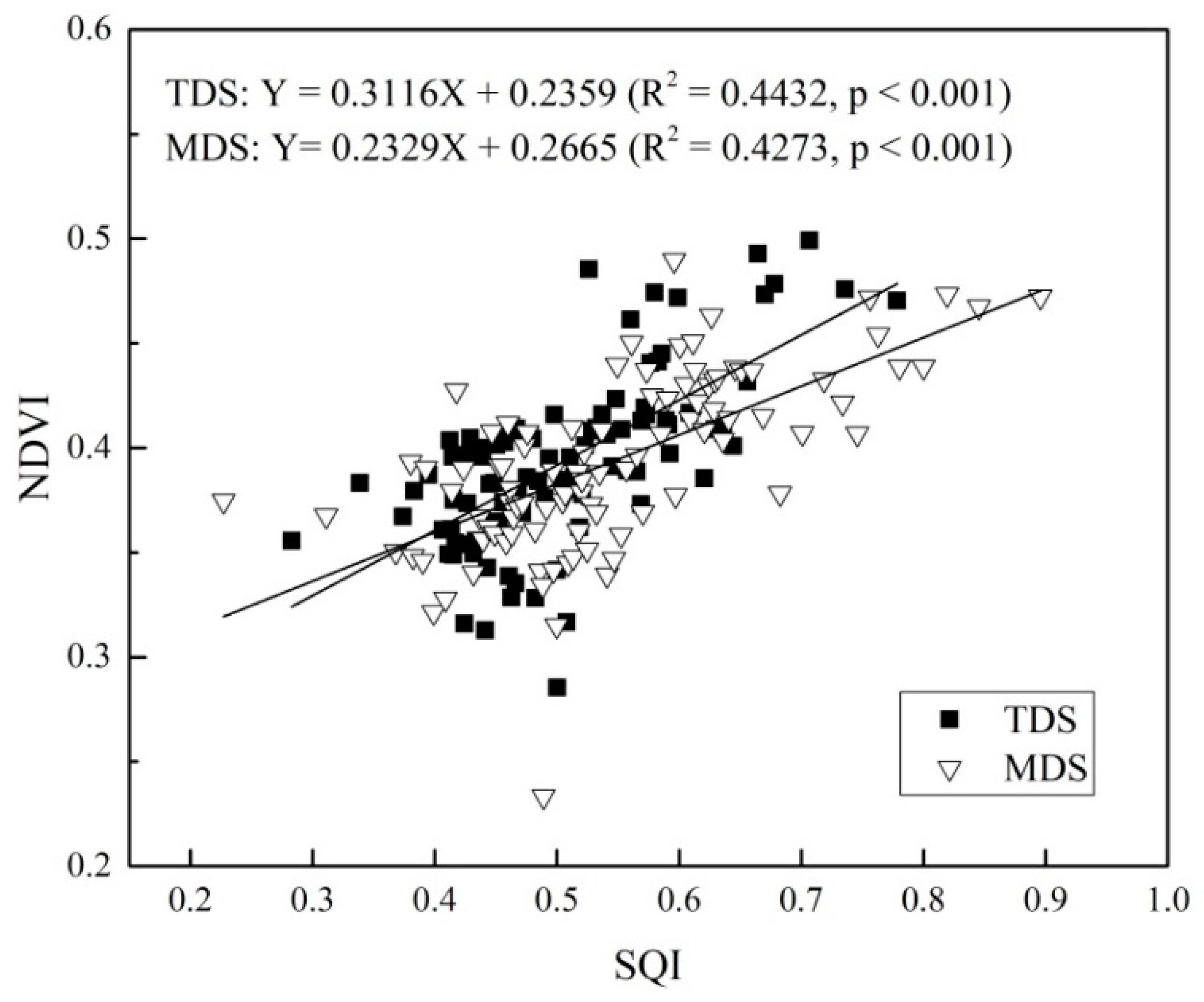
Figure 3.
Spatial patterns of soil quality in the Taihang Mountains. The SQI spatial distribution was illustrated for the evaluation results with TDS (a) and MDS (b).
Figure 3.
Spatial patterns of soil quality in the Taihang Mountains. The SQI spatial distribution was illustrated for the evaluation results with TDS (a) and MDS (b).

Figure 4.
Relative importance of the controlling factors in affecting SQI. See Table 1 for abbreviations.
Figure 4.
Relative importance of the controlling factors in affecting SQI. See Table 1 for abbreviations.

Figure 5.
The relationships between soil quality indices with the grades of five environmental factors, soil type (a), land cover (b), soil waster availability (c), elevation (d), and slope (e). One-way ANOVA was conducted within each environmental factor to test for differences among groups. Different letters above the error bars indicated significant differences between groups at p < 0.05, e.g., letters a–g for soil type (a), and it was the same with land cover (b), soil water availability (c), elevation (d) and slope (e). See Table 1 for abbreviations.


Table 1.
Data and corresponding abbreviation of environmental factors and soil properties.
| Variable | Data Sources | Category | Abbreviation |
|---|---|---|---|
| Land cover (LC) | [42] | Broadleaf forest | BF |
| Needleleaf forest | NF | ||
| Shrubland | SHL | ||
| Grassland | GS | ||
| Meadow | MD | ||
| Cropland | CL | ||
| Water | WT | ||
| Soil type (ST) | RESDC | Brown soils | BS |
| Cinnamon soils | CS | ||
| Castano-cinnamon soils | CCS | ||
| Loessial soils | LS | ||
| Neo-alluvial soils | NS | ||
| Lithosols | L | ||
| Skeletal soils | SS | ||
| Fluvo-aquic soils | FS | ||
| Water availability (WA) | MOD16A2 | ||
| Elevation (EL) | SRTM | ||
| Slope (SL) | elevation | ||
| Soil indicator | [39] | Clay fraction | CF |
| Bulk density | BD | ||
| pH value | pH | ||
| Organic matter fraction | SOM | ||
| Cation exchange capacity | CEC | ||
| Total nitrogen | TN | ||
| Total phosphorus | TP | ||
| Total potassium | TK | ||
| Alkali-hydrolysable nitrogen | AN | ||
| Available phosphorus | AP | ||
| Available potassium | AK |
Table 2.
Principal component analysis of soil properties for minimum data set (MDS) indicator selection.
Table 2.
Principal component analysis of soil properties for minimum data set (MDS) indicator selection.
| Soil Indicators | PC1 1 | PC2 | PC3 | PC4 |
|---|---|---|---|---|
| AK | 0.11 | −0.57 | −0.36 | 0.17 |
| AN | −0.32 | −0.15 | −0.35 | 0.29 |
| AP | −0.03 | −0.23 | −0.41 | −0.49 |
| BD | 0.15 | −0.45 | 0.29 | 0.41 |
| CEC | −0.433 | 0.07 | −0.05 | −0.11 |
| CF | −0.13 | 0.05 | −0.53 | 0.06 |
| pH | −0.35 | −0.09 | 0.37 | −0.28 |
| SOM | −0.422 | −0.30 | 0.17 | 0.00 |
| TK | 0.20 | −0.26 | 0.03 | −0.62 |
| TN | −0.42 | −0.33 | 0.17 | −0.02 |
| TP | 0.38 | −0.34 | 0.13 | −0.05 |
| Eigenvalue | 3.84 | 1.73 | 1.36 | 1.06 |
| Variance (%) | 34.86 | 15.70 | 12.40 | 9.61 |
| Cumulative variance (%) | 34.86 | 50.56 | 62.96 | 72.57 |
1 PC, principal component. 2 Underlined factor loadings are considered highly weighted. 3 Boldfaced factor loadings are the highest weighted loading in each principal component (PC). Underlined factor loadings correspond to the soil indicators included in MDS. See Table 1 for abbreviations.
Table 3.
Thresholds of each indicator for ideal soil standards.
| Thresholds 1 | AK (mg/kg) | AN (mg/kg) | AP (mg/kg) | CEC me/100 g | SOM (g/kg) | TK (g/kg) | TN (g/kg) | TP (g/kg) | BD (g/cm3) | CF (%) | pH |
|---|---|---|---|---|---|---|---|---|---|---|---|
| U | 200 | 150 | 40 | 200 | 40 | 25 | 2 | 1 | 1.45 | 28 | 9.0 |
| M | - | - | - | - | - | - | - | - | - | 20 | 7.0 |
| L | 30 | 30 | 3 | 50 | 6 | 5 | 0.5 | 0.2 | 1.10 | 8 | 4.5 |
1U, upper thresholds; M, optimum points; L, lower thresholds. See Table 1 for abbreviations.
Table 4.
Statistical analysis of the total area and the percentage for different SQI intervals.
| SQI Intervals | TDS | MDS | ||
|---|---|---|---|---|
| Area (km2) | % | Area (km2) | % | |
| I: <0.3 | 1145.53 | 0.84 | 1985.45 | 1.46 |
| II: 0.3–0.4 | 5707.92 | 4.19 | 10,915.55 | 8.02 |
| III: 0.4–0.5 | 71,549.05 | 52.58 | 40,771.50 | 29.96 |
| IV: 0.5–0.6 | 40,723.86 | 29.93 | 40,634.01 | 29.86 |
| I: 0.6–0.7 | 13,060.28 | 9.60 | 27,324.62 | 20.08 |
| VI: 0.7–0.8 | 3573.40 | 2.63 | 9753.01 | 7.17 |
| VII: 0.8–0.9 | 307.65 | 0.23 | 4541.97 | 3.34 |
| VIII: >0.9 | - | - | 141.57 | 0.10 |
Table 5.
Path analysis of soil quality with environmental factors.
| Factors | Correlation Coefficient | Path Coefficient | ||||||
|---|---|---|---|---|---|---|---|---|
| Direct Effect | Indirect Effect | |||||||
| ST | LC | WA | EL | SL | Summation | |||
| ST | 0.491 ** | 0.439 | 0.028 | 0.000 | 0.013 | 0.013 | 0.054 | |
| LC | 0.402 ** | 0.112 | 0.109 | 0.052 | 0.071 | 0.059 | 0.291 | |
| WA | 0.312 ** | 0.131 | −0.001 | 0.045 | 0.080 | 0.048 | 0.172 | |
| EL | 0.340 ** | 0.153 | 0.037 | 0.052 | 0.068 | 0.040 | 0.197 | |
| SL | 0.331 ** | 0.116 | 0.050 | 0.057 | 0.054 | 0.053 | 0.214 | |
**—the correlation coefficient is significant at 0.01 level based on F-test. See Table 1 for abbreviations.
© 2018 by the authors. Licensee MDPI, Basel, Switzerland. This article is an open access article distributed under the terms and conditions of the Creative Commons Attribution (CC BY) license (http://creativecommons.org/licenses/by/4.0/).
Share and Cite
MDPI and ACS Style
Geng, S.; Shi, P.; Zong, N.; Zhu, W. Using Soil Survey Database to Assess Soil Quality in the Heterogeneous Taihang Mountains, North China. Sustainability 2018, 10, 3443. https://doi.org/10.3390/su10103443
AMA Style
Geng S, Shi P, Zong N, Zhu W. Using Soil Survey Database to Assess Soil Quality in the Heterogeneous Taihang Mountains, North China. Sustainability. 2018; 10(10):3443. https://doi.org/10.3390/su10103443
Chicago/Turabian StyleGeng, Shoubao, Peili Shi, Ning Zong, and Wanrui Zhu. 2018. "Using Soil Survey Database to Assess Soil Quality in the Heterogeneous Taihang Mountains, North China" Sustainability 10, no. 10: 3443. https://doi.org/10.3390/su10103443
Note that from the first issue of 2016, this journal uses article numbers instead of page numbers. See further details here.