Computer-Based Analysis of the Stochastic Stability of Mechanical Structures Driven by White and Colored Noise


Department of Engineering, German University of Technology in Oman, Muscat, PC 130, Oman
Sustainability 2018, 10(10), 3419; https://doi.org/10.3390/su10103419
Submission received: 4 August 2018
/
Revised: 19 September 2018
/
Accepted: 22 September 2018
/
Published: 25 September 2018
(This article belongs to the Special Issue Modelling and Analysis of Sustainability Related Issues in New Era)
Abstract
:The goal of this paper is to design an effective Proportional Integral Derivative (PID) controller, which will control the active suspension system of a car, in order to eliminate the imposed vibration to the car from pavement. In this research, Gaussian white noise has been adopted to model the pavement condition, and MATLAB/Simulink software has been used to design a PID controller, as well as to model the effect of the white noise on active suspension system. The results show that the designed controller is effective in eliminating the effect of road conditions. This has a significant effect on reducing the fuel consumption and contributes to environment sustainability.
1. Introduction
1.1. Background
Efforts to optimize fuel consumption have driven and inspired various industries, including the automobile industry, to create a wealth of new inventions and technologies. Since the issue of global warming was brought into the spotlight, the mechanics of the automobile industry have evolved rapidly, due to the greenhouse gas emissions produced by internal combustion engines. The advancement of technology within the power industry have helped in reducing fuel consumption, as well as in the reduction of greenhouse gas emissions [1].
Greenhouse gases released by vehicles include carbon dioxide, carbon monoxide, nitrogen dioxide, ozone and methane, among others. The repercussions of burning fossil fuels amount to more than just a foul smell; the aftermath of these greenhouse gases impacts the health of humans, animals and plants alike, thus disturbing the environment and its inhabitants [2]. Within the environment, greenhouse gases disrupt the biogeochemical cycles that exist in nature resulting in problems, such as temperature rise, erosion, and droughts. One problem is the melting ice caps; even a minute temperature rise can result in rising water levels, which also increases the number of natural disasters occurring in various areas. A rise in water levels also promises depletion in land mass, due to water levels overflowing, and swallowing coastal areas. Furthermore, car emissions, along with many by-products of plants, cause the radiation from the sun to be trapped inside the Earth’s atmosphere, resulting in the overall raising of the temperature. The aforementioned consequences develop into bigger problems, such as those which can already be observed in the La Nina and El Nino phenomena, and events in the Atlantic, as well as increased cyclone activity in the Indian Ocean [3].
Regarding the impact on humans, these greenhouse gases play an important role in the climate change that is affecting the entire globe (global warming), and may threaten the welfare of humans—physically and economically. For example, when ozone levels increase in lower elevations, it can have a direct impact on human health, including harming the respiratory system. The economy can also be affected, because of individuals who suffer from health problems caused by these issues. Furthermore, as the automobile industry grows, the use of fossil fuels will grow exponentially, bringing closer the possibility of a future with no fossil fuels, which will result in the economic downfall of bigger entities such as countries. Other greenhouse gases, such as fluorinated gases, do not interfere directly with human health, but do hurt the environment greatly, and on different levels [4].
Due to the rate at which fossil fuels are used annually (11 billion tons of oil and four billion tons of crude oil, per annum), oil deposits on Earth are predicted to run out by 2052. Furthermore, compensating the energy deficit of the oil deposits through using natural gas will only extend the lifetime of fossil fuel energy by an additional eight years. After this, the only remaining form of fossil fuel energy left would be coal. To fill in the energy gap of both the oil and natural gas deposits, coal would be so extensive we run out of fossil fuels by the year of 2088 [5]. Fossil fuels have, thus far, been the main source of energy, but with the passing of time, different sources of energy alternatives have been developed to prevent the consequences that arise from using just fossil fuels. For instance, instead of having only internal combustion engine vehicles, there are a variety of eco-friendly vehicles available, which are being used instead. Some of these eco-friendly energy sources include electronically powered vehicles, hybrid vehicles (using more than one source of energy), compressed air, etc. [6]. There are many of problems that come with the use of fossil fuels, out of which the issues with the greatest impact are its scarcity and the cost it imposes on the planet. Fossil fuels are the only plausible option for many vital functions and processes; the most important of these is transportation. Therefore, using this source of energy wisely and as efficiently as possible is a must [7].
1.2. Factors Effecting Fuel Efficiency
Fuel efficiency can be described as how well the chemical energy of the fuel in question is converted into kinetic energy, in terms of powertrains. Fuel efficiency varies according to several factors, including the application, the size of the vehicle, the vehicles design, power, engine parameters, and many others. Factors that affect fuel consumption are design-related, environment-related, and motorist driving strategy-related factors. Together, and individually, these factors determine how much energy needs to move the vehicle [8,9].
1.2.1. Vehicle Design Factors
To design a vehicle with the lowest fuel consumption rate (irrespective of the energy source) is one of the main goals of modern car manufacturers. Car manufacturers have expended great effort on developing, and successfully applying, different approaches to a vehicle’s design (especially the vehicle’s size) in order to reduce its fuel consumption, as well as the harmful gases emitted. There are several parameters falling under this design category, including the aerodynamic drag, engine parameters, rolling resistance, load, and fuel type. The size of the engine refers to how much fuel can be pumped into the engine, in order to be burned and converted into energy. Meaning, the larger the capacity of the engine, the more power the car has (although that over simplifies the concept). When a car has an engine with a capacity of two liters for instance, this means that the total amount of fuel that can fit into the cylinders is two liters, regardless of the number of cylinders. That power is measured in horse power, or brake horse power [10,11].
In terms of fuel efficiency, a bigger engine does not always mean worse fuel economy. For instance, a car with a larger engine running at a high speed for a long time will use less fuel than a car with a smaller engine running at the same speed for the same length of time. Furthermore, considering recent technology, it is now made possible for a large engine, of for example six cylinders, to use only three cylinders when that is all that is needed, therefore greatly boosting fuel efficiency [12].
The aerodynamic aspect of design is concerned with improving the cars exterior to better tackle drag, and to cause lower resistance at higher speeds. At a speed of 50 km/h, the power needed from the engine to overcome air friction is not more than 40% of the engine’s power, yet when it comes to speeds greater than 80–90 km/h, the power needed increases to 60%, and more of the engine’s power. This is due to drag increasing proportionally to the square of the speed, and the power needed is proportional to the cube of the speed [13].
Rolling resistance, or rolling friction, is the resistance against the motion of a tire when rolling on a certain surface. Three forms of rolling resistance are in question, namely; permanent deformation, hysteresis losses, and slippage between the surface and the tire. Interestingly, a worn-out tire gives lower rolling resistance than a new one, due to the depth of the tread on the tire and its friction inducing properties—which in turn, leads to lower fuel consumption. Hysteresis losses are the main reason for rolling friction. Because tires are made of a deformable material, the tire is subject to repeated cycles of deformation and recovery, there is energy dissipated as heat. The energy is lost basically when the energy of healing/recovery is less than that of the deformation. Because of rubber’s properties, it does not recover or heal over a short period of time—it needs a longer time. Some manufacturers include silicone in the tread of the tires to cut down on the time needed for the tire to recover, and hopefully cut down on the lost energy rates [14,15].
Fuel type also influences fuel consumption. A diesel engine delivers better fuel economy for several reasons—the main reason being that diesel contains higher energy content than gasoline. However, that does not mean it affects performance in terms of speed—it instead delivers more power and torque, which is why most trucks have diesel engines. When comparing a diesel engine to a gasoline engine, the difference in fuel economy shows the diesel engines to be 25–30% more fuel economic, and in some cases, up to 40% more economic. The obvious cut back to using a diesel engine is speed in terms of performance, on the other hand, when compared to a gasoline engine of the same size; more economic [16]. A diesel-powered engine is a very sophisticated one and, in a sense, more delicate than a gasoline powered engine. For example, if water somehow gets into the fuel tank (whether it is the suppliers fault or a combination of heavy rain and bad luck), it could lead to many problems, including the most obvious one—severe damage to the engine [17,18].
The load on the vehicle is another factor that affects fuel economy of car. When a vehicle is overloaded, the power it requires increases. This is because the engine will need to produce more power to move the vehicle at any given speed, in addition to the increased load on the tires, which in return, increases rolling resistance (which also increases fuel consumption) [19].
1.2.2. Environmental Factors
The weather and climate influence the fuel economy of cars—although not drastically. In the winter for example, the air is heavier and denser, therefore the air drag coefficient is larger. The tires experience a decrease in pressure which decreases fuel economy. Lubricants, wherever they may be, become cold and harder, and interfere with fuel economy, as well due to the increase in friction. In the summer however, the air is lighter and less dense, making it easier to navigate in contrast [20].
The terrain in which a car travels can influence its fuel consumption in a positive or negative manner. Rough terrain, ascents, slippery surfaces, sandy/muddy surfaces, and other types of terrain affect fuel consumption negatively. The opposite of these terrains can either not affect the fuel consumption or even affect it positively. For instance, climbing up a hill requires a significantly more power (which means burning more fuel), while descending a hill requires little or no fuel to be used [21].
Driving within a city uses much more petrol per km when compared to driving on a highway or in the country side. The reason for this that there are limitations and conditions that exist in the city, but not outside it or on the highway; such as traffic, speed bumps, more turns, pedestrians, etc. When driving in the city, the driver must use their brakes a greater number of times, decreasing fuel economy. Another active factor is the fact that in the city, the driver is forced to drive at lower speeds. Speeds lower than the optimum speed also affect fuel consumption, and significantly more when combined with the reasons mentioned. When driving on the highway or the countryside, the limitations faced in the city are either not faced, or significantly lower. The vehicle is much more likely to be driven at optimum speeds, leading to a better fuel consumption rate [22,23,24].
1.3. Formulation of the Problem
One of the important factors which has a great influence on fuel consumption of transportation vehicles is pavement condition [25]. It is a fact that, due to the interaction between tire and the pavement, the tires of a vehicle partially deform; this deformation results in the stored potential energy of the tires being converted to heat, which is partly absorbed by the rest of tire, with the remainder being dissipated into the atmosphere [26]. Therefore, it is important to know that higher pavement texture results in more fuel consumption [27]. In past decade, due the problem of global warming and drawbacks of high consumption rate, modelling and simulating the effect of different type of pavement conditions on fuel consumption rate, and its effect on environment, has been a topic of interest for many researchers [28,29,30,31,32]. Interestingly, the results have continuously shown that pavement smoothness has the highest impact on the rate of fuel consumption: The smoother the road, the less fuel consumption [33,34,35,36].
There is also energy loss during vehicle transportation on the road. Energy is absorbed and converted to a thermal energy form, by the suspension system and tires, meaning energy loss will be reduced if the suspension system can eliminate the effect of the pavement condition, and make vehicle bounces less [37]. Therefore, designing an effective suspension system to compensate the effects of pavement conditions on vehicle is a way to reduce fuel consumption.
1.3.1. Methods of Improving the Fuel Efficiency
One of the ways to decrease the load/mass of the car is through choosing high-tech materials, as to increase fuel efficiency without jeopardizing the safety of the passenger. Some automakers are trying to use plastic fuel tanks and carbon fiber instead of steel. Alas, carbon fiber, a lightweight and reliable material, is unlikely to be used, due to its hefty price in the market. A record by the EPA (Environmental Protection Agency), shows that for every 45 kg of mass reduced, fuel efficiency can increase by one to two percent (1–2%) [38,39].
Modifying the engine appropriately (e.g., adding/improving a turbo charger) can improve efficiency of fuel consumption by up to 4%, and fixing a serious problem (such as a broken oxygen sensor) can improve efficiency by a staggering 40%. Keeping the pressure of the tires in check (at the adequate pressure accordingly) improves fuel consumption by up to 3.3%. Old cars that use a carbureted engine are still in use and by keeping their air filters unclogged could help with fuel economy and acceleration. In more modern cars however, it usually aids with acceleration only [40,41,42].
One crucial step in optimizing fuel efficiency involves developing analytical models to predict the vehicle’s fuel consumption and to achieve the desired results. There have been models that compute fuel consumption estimates in cars, with respect to their fuel consumption, characteristics and the surrounding environment. However, these models only represent approximations to these estimates. By adding more variables to the models, the outcomes will become more accurate—but this will result in a less efficient model. This is because mathematical models represent approximations to the real result, while having errors in each of the parameters used. Therefore, the more parameters one uses, the more errors are involved, thus making the model less efficient [43].
There have been many attempts to enable mathematical models to predict fuel consumption, with different variables in each. The first time metrics mathematical models were utilized to predict vehicle fuel consumption and emissions was by Ahn et al. [44]. The proposed model is a function of speed and acceleration, with constant parameters, and can predict fuel consumption or CO emission rates for an assumed vehicle. According to Ross et al. [45] there are two factors that affect vehicle fuel consumption: The efficiency of the powertrain, and the power required in working the vehicle. He evaluated fuel consumption by finding the product of optimal specific fuel consumption into the sum of the powers of the rolling resistance, air resistance, and inertial acceleration resistance, and then dividing it by the product of the efficiency of transmission with the average speed of the vehicle and the fuel density. In another research, on analytic modelling of vehicle fuel consumption, it has been shown that the fuel consumption can be found by using the calorific value of fuel per 100 km [43]. This was done by finding the sum of energies of the forces required to overcome resistance and the kinetic energy required for episodic accelerations, and then dividing it by the calorific value of the fuel used. In 2008, Smit et al. [46] conduct a study which examined how, and to what extent, models used to predict emissions and fuel consumption from road traffic, including the effects of congestion. In 2011, Rakha et al. [47] developed a fuel consumption model which can be easily integrated within a traffic simulation framework. In 2015, Tang et al. [48] proposed a model to investigate the impacts of the driver’s bounded rationality and the effect of signal lights on the fuel consumption. In 2017, a fuel consumption model for heavy duty tracks has been proposed by Wang et al. [49].
1.3.2. Methods of Improving the Vehicle Suspension
From the point of view of ride safety, the most important element of the vehicle (which has a direct impact on passengers comfort) is the suspension system [50]. Nowadays, with advancements in the car manufacturing industry, companies attempt to provide a smooth ride for passengers through the development and manufacture of more advanced vehicle suspension systems. These systems are able to minimize the effects of uneven pavement conditions of roads on the passengers [51]. In 2016, Kognati et al. [52] proposed a unified approach to model complex multibody mechanical systems, and design controls for them. Pappalardo et al. [53], in 2017, proposed a novel methodology to address the problems of suppressing structural vibrations, and attenuating contact forces, in nonlinear mechanical systems; and in 2018 they developed an adjoint method—which can be effectively used for solving the optimal control problem, associated with a large class of nonlinear mechanical systems [54]. Nowadays, to optimize the quality of travel by cars, various types of controllers (such as adaptive control [55], Linear Quadratic Gaussian (LQG) control [56], H-infinity [57], Proportional (P) controller [58], Proportional Integral (PI) controller [59], and Proportional Integral Derivative (PID) controller [60]) have been utilized, in order to control the car suspension system and to eliminate the vibration coming from the pavement. In 2014, Li et al. [61] proposed an output-feedback H∞ control for a class of active quarter-car suspension systems with control delay. In 2015, AENS et al. [62] performed a Comparison between passive and active suspensions systems. In 2016, Buscarino et al. [63] investigated the role of passive and active vibrations, for the control of nonlinear large-scale electromechanical systems, which have also been investigated by Zhao et al. [64], in 2016, who utilized adaptive neural network control for an active suspension system with actuator saturation. Taskin et al. [65], in 2017, investigated the effect of utilizing fuzzy logic controller on an active suspension system based on a quarter car test rig; and in 2018 a control scheme, utilizing Hybrid ANFIS PID, was proposed by Singh et al. [66], in order to improve the passenger ride comfort and safety in an active quarter car model. Furthermore, Fauzi et al. [67], in 2018, developed a state feedback controller to reduce body deflection caused by road disturbance, to achieve the ride comfort of driver and passengers.
1.4. Scope and Contribution
The goal of this paper is to design an effective PID controller, to control the active suspension system of a car, in order to eliminate the imposed vibration to the car from pavement, which has a major role in the fuel consumption rate. In this research, the Ahn mathematical model has been utilized to model the fuel consumption rate, and Gaussian white noise has been adopted to model the pavement condition. The logic behind selection of this type of noise is the randomness property of it. Generally, the term noise or random fluctuations characterize all physical systems in nature. The apparently irregular or chaotic fluctuations were considered as noise in all fields, except in a few, such as astronomy [68].
The term “white” refers to the frequency domain characteristic of noise. Ideal white noise has equal power per unit bandwidth, which results in a flat power spectral density across the frequency range of interest. Therefore, the power in the frequency range from 100 Hz to 110 Hz is the same as the power in the frequency range from 1000 Hz to 1010 Hz. The term “Gaussian” refer to the probability density function (pdf) of the amplitude values of a noise signal. The color of the noise refers to the frequency domain distribution of the noise signal power. Since the white noise contain all frequencies, it can be considered as random input, which simulates the any type of pavement condition. In this case instead of simulating the road conditions with different color noises simply the Gaussian White Noise can be utilized [69].
In this research, MATLAB/Simulink software has been utilized to model the fuel consumption rate, to design a PID controller and to model the effect of the white noise on the quarter car suspension system. The results show that the PID controller has an effective performance to eliminate the effect of road conditions and reducing the fuel consumption rate which has a significant effect on environment sustainability.
1.5. Organization of the Paper
After the brief introduction the rest of the manuscript has been organized in following manner. First, in Section 2 (Methodology), the fuel consumption mathematical model, steps of simulation set up and data collection have been described in detail. Then in Section 3 (Results), the proposed methodology has been verified by analyzing the results. Finally, in Section 4 (Conclusions and Future Work) the summary of the manuscript has been provided, and possible future works have been suggested.
2. Methodology
Vehicle handling performance and fuel consumption rate are two important factors which are directly affected by vehicle suspension system [70]. Conventionally, in order to decrease the vehicle vibration a combination set up of springs and dampers has been used. This set up is generally known as passive suspension system. The input disturbance to the car from pavement condition cannot be eliminated by passive suspension system, since the damping ratio is constant and not adjustable. To eliminate the effect of the road condition, the best solution is to utilize an autonomous control system, known as active suspension system, which can compensate for the noise input to the system by exerting force to the system [71].
In this paper, the problem has been defined as how an effective controller can be designed to control an active suspension system, to eliminate the pavement condition effects to reduce the fuel consumption. To fulfil the task first in next section, the Ahn fuel consumption mathematical model has been introduced, to model the fuel consumption rate before and after utilizing the PID controller. Next, an active suspension system has been introduced, and later, with respect to the control engineering concept, the introduced active suspension system mathematically has been modelled. In this third stage, the effect of the pavement condition on the vehicle, introducing the white noise concept, has been modelled, and in the next step, a PID controller (to control the proposed active suspension system) has been designed. In fifth step, the proposed system has been simulated, utilizing MATLAB-Simulink. This is followed by a performance analysis of the controller, and finalized by investigating the stability of the proposed controller.
2.1. Fuel Consumption Model
As discussed previously, there have been several different approaches taken to model the fuel consumption in a vehicle. Some of these approaches could be similar in terms of using the same variables but might have a different mathematical representation of the data, while others would have different variables all together with or without the same mathematical model. Most of the researches led in this field do not include every variable affecting the outcome of a vehicle’s fuel consumption. This is due to a reason mentioned previously, regarding the decrease in the efficiency of the model. Because of this specific reason, the research conducted usually involves a limited number of variables.
In this article, the Ahn mathematical model has been utilized to calculate the fuel consumption rate. As shown in Equation (1), the model uses a vehicle’s speed and acceleration alongside constants to find a vehicle’s fuel consumption [72]:
where F is the rate of fuel consumption measured in (lit/h) as a function of a vehicle’s speed and acceleration; y being the vehicle’s speed measured in m/s; and x the acceleration measured in m/. The letters a to p are constants with the following values: a = −0.67944; b = 0.135273; c = 0.015946; d = −0.00119; e = 0.029665; f = −0.00028; g =1.49 × 10⁻⁶; h = 0.004808; i = −2.1 × 10⁻⁵; j = 5.54 × 10⁻⁸; k = 8.33 × 10⁻⁵; l = 9.37 × 10⁻⁷; m = −2.5 × 10⁻⁸; n = −6.1 × 10⁻⁵; o = 3.04 × 10⁻⁷; p = −4.5 × 10⁻⁹.
2.2. Active Suspension Model
In this paper, the quarter car dynamic vibration model has been chosen to represent the active suspension model (see Figure 1). While this model has limitations, such as eliminating vehicle’s pitching and roll angle vibrations, it also includes the most essential features for this research, such as the change of the load and suspension system’s stress information, which has been utilized by many researchers, to investigate the effect of pavement conditions on body vibration of a vehicle [73,74,75,76,77].
As shown in Figure 1, the vehicle body mass (known as the sprung mass) has been shown with M1, and the mass of the axel and wheel, which has been shown with M2, represents the unsprung mass. The tire is assured to maintain contact with the surface of the road when the vehicle is traveling, and is modelled as a linear spring with stiffness K2. The linear damper, which average damping coefficient is D, and the linear spring, which average stiffness coefficient is K1, consist of the passive component of the suspension system. The vertical displacements of the M1 and M2 respectively have been represented by the state variables X0(t) and X2(t), since vertical pavement condition has been shown by X1(t). The active control force which has been created by the active suspension actuator is shown by U.
Generating a mathematical model is the first step of modelling a system, followed by calculating the design parameters. In an control engineering field, a system can be modelled mathematically in three different ways: (1) State space description; (2) transfer function description; and (3) weight function description [78].
In this paper, the active quarter car suspension model (which has been presented in Figure 1) has been modelled mathematically by the Transfer Function method. To fulfil the task, two degrees of freedom motion differential equations have been generated (Equations (2) and (3), as follows), by analyzing the vehicle suspension system dynamics (Figure 1):
One must assume that all of the initial conditions are zero, so these equations represent a situation when the wheel of a car goes over a bump. The dynamics of Equations (2) and (3) assume that all initial conditions are zero, and there can be expressed in the form of transfer functions by taking Laplace Transform of the equations. This is to represent the condition of when vehicle goes over a bump. It is important to know that the system will have two transfer functions, as represented in Equations (4) and (5):
where
G1(s) represents the effect of exerted force, on the vertical displacement of the car, which has been produced by active suspension system; and G2(s) represents the effects of the pavement condition on the vertical displacement of the car.
This means that vertical displacement of the vehicle is superposition of the effects of both active suspension force and pavement condition. As mentioned in previous section, the goal of this research is to eliminate the effect of pavement condition on the system by utilizing a controller (in other words, this article proposes that, by adjusting the produced force by active suspension, the effect of the road condition can be eliminated). To achieve this goal, a PID controller, proposed and explored in next section, in order to control the amount of the produced force.
2.3. PID Controller
A PID controller is a closed loop controller type, which controls the plant output variable by minimizing the error between real plant output, and desired output. A PID controller consists of three controller modes: P as proportional controller, I as integral controller; and D as derivative controller (see Figure 2) [79].
In industrial control systems, the main mode of the PID controller, are mostly known as the proportional control mode—which determines the controller response to the plant error by multiplying the error to the P controller’s gain (Kp), so that a higher Kp will result in higher P action to the plant error (see Equation (7)) [80].
The effect of the integral controller mode can be defined as decreasing, or increasing, the response time of the controller to the plant error, by calculating the integral of the error, and multiplying it to the I controller’s gain (KI), so that a higher KI will result in higher I action to the plant error (see Equation (8)) [81].
The last mode of a PID controller, which regulates the plant’s output by calculating the derivative of the error and multiply it to the P controller’s gain (KD), is derivative controller mode (see Equation (9)). The D mode controllers are widely used in motion control systems, since they are very sensitive against of noise and disturbances [82].
It is important to know that a PID controller is the weighted sum of these three modes of control, and based on the plant requirements, one or two modes can be eliminated. The response of the PID controller, control signal u(t), to the plant error can be determined, as shown in Equation (10) [83].
It is highly important to mention that knowing effect of the each of these three modes on the response of the controller is an essential criteria in control theory; and any change in PID controller’s coefficients can result in changing the status of the system from stable to unstable (see Table 1) [83].
As seen in Table 1, if the Kp is increased too much, the control loop will begin oscillating, and become unstable. Furthermore, the system will not receive desired control response if Kp is set too low. The similar rules exist for integral and derivative controller modes.
The controller response will be very slow if the integral time is set too long, and system will be unstable the control loop will oscillate if KI is set too low. However, if KD increases too much, then oscillations will occur, and the control loop will turn to unstable.
By knowing the active suspension model and PID controller concept, the next step is design an effective PID controller for the quarter car model.
The goal of this paper is to design an effective controller by eliminating the effect of the pavement on the vehicle passengers. The controller should be designed to make its system stable, by eliminating the disturbance of the road, which shows itself as an oscillation of the vehicle; and, at the same time, has a smooth and fast control signal to ensure that passengers comfort and safety are not compromised. PID controllers are one of the best controllers that can be utilized for this purpose, since they are capable to reach the steady state error by having a short rise time, and they can give stability to a system by eliminating oscillations and overshoot of the system.
The proposed PID controller in this paper consists of all three controller modes: Proportional, integral and derivative. The proposed controller is capable of eliminate the noise of the pavement by adjusting the force of proposed active suspension system (see Figure 3).
It is important to know that how the proposed PID controller works.
As mentioned previously, in this research, the effect of the exerted force on the vertical displacement of the car, produced by active suspension system, has been mathematically modelled as G1(s). The input of this mathematical model is the PID controller output, which results in the displacement of body of the vehicle (sprung mass), with respect to the unsprung part. However, there is one more element which affects this displacement, such as the pavement condition. The road condition shows its effect as disturbance on the system, and, in this paper, it has been modelled mathematically as G2(s).
Since the reference input should be equal to zero, so it can be concluded that the difference between the reference input and total displacement, which is known as error function E(s), is the superposition of the effects of the control signal and noise signal on vehicle. In this case, the PID controller adjusts the active suspension force by calculating each mode signal, based on the error function E(s) (see Figure 4).
The proposed PID controller for the modelled quarter car’s active suspension system has been simulated in a MATLAB-Simulink environment. The simulation’s performance is based on the parameters found in Table 2.
3. Results
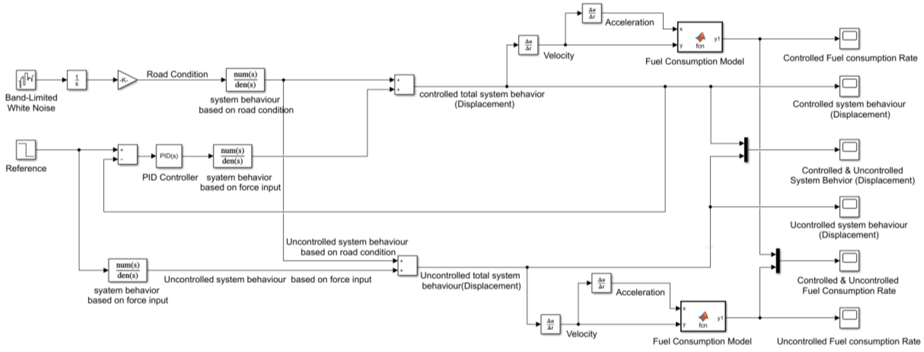
As seen in Figure 5, the proposed methodology has been implemented and modelled in a MATLAB-Simulink environment. The model can be dived in two main parts: (1) Controlled parts; and (2) uncontrolled parts. The controlled part consists of the proposed PID controller, to reduce the effect of the imposed fluctuations by the pavement condition on the vehicle, and the effect of the controller on reduction of the fuel consumption rate. The uncontrolled parts consist of the effects of the pavement conditions on a vehicle’s vertical displacement, and the effect of these vibrations on the fuel consumption rate. The pavement condition x0(s) has been modelled by Gaussian white noise. The reason is that the road unevenness is kind of noise, which should be compensate—therefore, any kind of colored noise such as pink, red, green, etc., can be utilize for this purpose [84]. Since white noise contains all frequencies of colored noises, so it is a good approximation to simulate the randomness of pavement roughness [85].
As seen in Figure 5, the reference input (which here is the desired output) has been simulated by the step function. The reason is that the reducing and even elimination the vehicle oscillations is desirable, and the oscillations is resulted by displacements of sprung mass, with respect to unsprung mass. The displacement has been calculated as plant’s output (x0(s) − x2(s)). Since the target is to eliminate it, the desired output should be considered as zero, and a step function (generating zero value at t > 0) is a good model to generate the required data.
The effect of the random road pavement, which has been modelled by a Gaussian white noise generator, has been illustrated in Figure 6. It can be observed that the vehicle follows the road condition, with fluctuates with road fluctuations (which can be considered as unstable behavior). This will result in increasing fuel consumption, decreasing effective life of the vehicle’s part, and compromising passengers’ safety.
As seen in Figure 6, this uncontrolled response is not convenient for the passengers. Therefore, in order to reduce and eliminate the effect of the road pavement on the car, which shows itself as car fluctuation (as described before), a PID controller has been designed.
By utilizing the PID controller, as it can be observed from Figure 7, the car does not follow the road condition, and the active suspension controller cancels out the unpleasant pavement condition’s effect on the car.
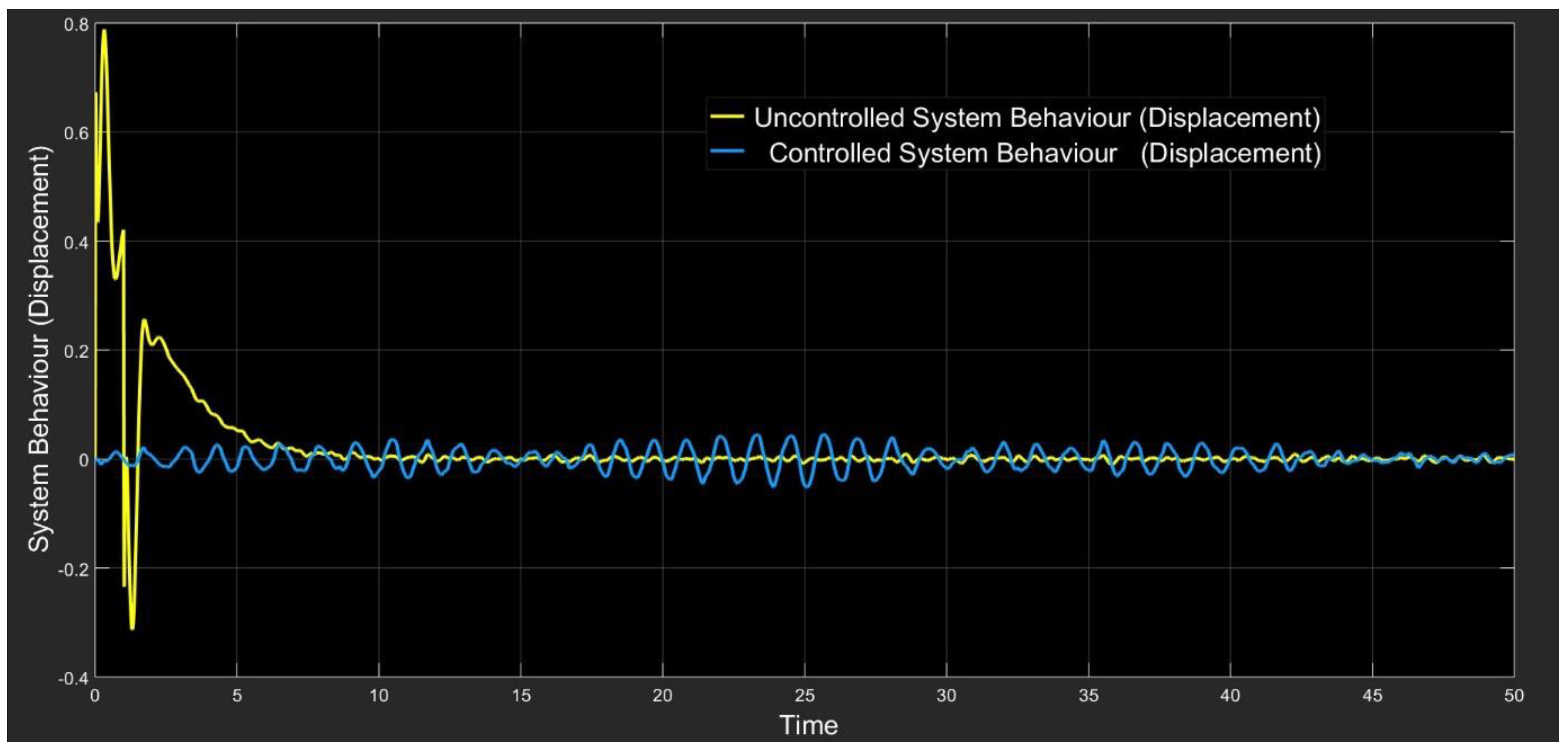
To have a better understanding of how the proposed PID controller compensate for the effect of the pavement, controlled and uncontrolled total system behaviors have been shown in Figure 8. As can be observed, the first system shows an aggressive controlled response to the input noise, but after three seconds it starts to cancel the noise, and prepares a convenient and safe ride for passengers.
As seen in Figure 5, in the proposed model, two fuel consumption blocks have been created to calculate the changing of the fuel consumption rate. It is important to mention that the mathematical model, inside both blocks, is the Ahn model, which has been discussed previously. The fuel consumption model, in the lower part of the model, has the role of calculating the change of the fuel consumption rate, based on the imposed vibration by the road conditions on the vehicle. It is essential to remembered that here the proposed model is not capable of calculating the fuel consumption rate, since it should be calculated via horizontal displacement of the vehicle, but the vertical fluctuations act as a resistant in front of the engine acceleration. This means that the function of the block is simulating the uncontrolled change in fuel consumption rate.
The results, as shown in Figure 9, indicate that since speed and velocity of the vehicle are changing, during the simulation time, and the fuel consumption’s model depends on these two variables, the fuel consumption rate changes under the random pavement conditions, which results in more CO emissions.
As it is shown in Figure 10, after adding the proposed PID controller to the system, the fuel consumption rate at the beginning of the simulation, and at the first control signal, has a change—but it remains without any changes during the rest of the simulation period.
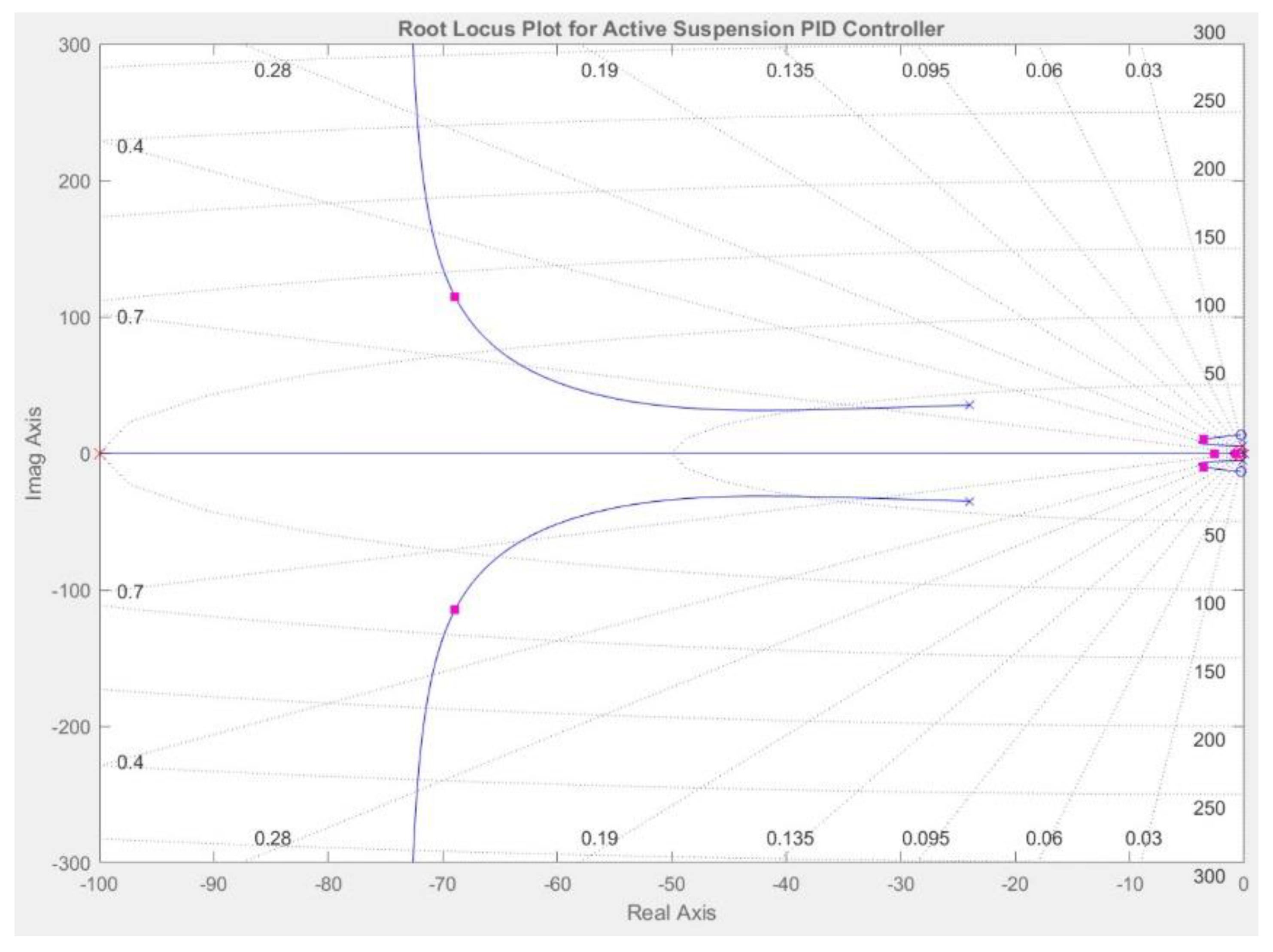
To explore the stability status of the designed controller in this research, as it can be seen in Figure 11, the compensator editor tool of the MATLAB software has been adopted. The system, without considering the forced step function input, has only one negative pole at −100, and two complex zeroes at −0.405 ± 1.19i. If the forced input effect is desired for consideration, another pole in zero has to be added to the system. Since the system only has a one negative pole, it can be concluded that the designed PID controller (based on the location of the poles) is a stable system, and (based on the location of the zeros) it has a damping ratio of 0.3, and a natural frequency of 1.25 Hz.
Now, by knowing the locations of the pole and zeros of the system, the Root Locus diagram can be plot. As seen in Figure 12, it can be concluded that by moving to the left side of the real axis, the system shows more stable behavior.
4. Conclusions and Future Work
The main role of a suspension systems is to reduce fuel consumption, and to unsure passenger safety. Road roughness yields fluctuations of the vehicle wheels, which is transmitted to the all parts of the vehicle, as well as the passengers. It becomes clear that the role of the suspension system is to reduce as many of these vibrations and shocks, which occur while driving, as possible. An effective suspension system should result in a smooth driving, with less vehicle vibrations, and a degree of comfort, based on the interaction with bumpy road surface. The vehicle behavior should not consistent of large oscillations in presence of a good suspension system. To achieve this goal, in this paper, an active car suspension has been modelled, and an effective PID controller has been proposed and designed, to cancel the negative effects of the pavement conditions. Since the Gaussian white noise produces random outputs, it has been adopted to simulate the pavement effects on the vehicle. The Ahn mathematical model was utilized to simulate the change of the fuel consumption rate—both in controlled, and uncontrolled conditions. Proposed plant and control architecture has been modelled by using the MATLAB-Simulink software package, and the stability of controller has been investigated. The results show that the proposed PID controller works, and has is effective, which in turn results in the decrease of fuel consumption, and prevents premature damage to the vehicle. For future studies, rather than the proposed linear model, nonlinear elements can be considered for the quarter car model, and the PID controller’s coefficients can be optimized by Ring Probabilistic Logic Neural Networks (RPLNN) Hybrid Algorithms, Genetic Algorithm, and other artificial intelligent techniques.
Funding
This research was funded by [The Research Council of Oman (TRC)] grant number [ORG/CBS/14/008].
Conflicts of Interest
The author declares no conflict of interest.
References
- Hoffert, M.I.; Caldeira, K.; Benford, G.; Criswell, D.R.; Green, C.; Herzog, H.; Jain, A.K.; Kheshgi, H.S.; Lackner, K.S.; Lewis, J.S.; et al. Advanced technology paths to global climate stability: Energy for a greenhouse planet. Science 2002, 298, 981–987. [Google Scholar] [CrossRef] [PubMed]
- Vitousek, P.M.; Mooney, H.A.; Lubchenco, J.; Melillo, J.M. Human domination of Earth’s ecosystems. Science 1997, 277, 494–499. [Google Scholar] [CrossRef]
- Dong, B.; Sutton, R.T.; Scaife, A.A. Multidecadal modulation of El Nino–Southern Oscillation (ENSO) variance by Atlantic Ocean sea surface temperatures. Geophys. Res. Lett. 2006, 33. [Google Scholar] [CrossRef]
- Younger, M.; Morrow-Almeida, H.R.; Vindigni, S.M.; Dannenberg, A.L. The built environment, climate change, and health: Opportunities for co-benefits. Am. J. Prev. Med. 2008, 35, 517–526. [Google Scholar] [CrossRef] [PubMed]
- Pacala, S.; Socolow, R. Stabilization wedges: Solving the climate problem for the next 50 years with current technologies. Science 2004, 305, 968–972. [Google Scholar] [CrossRef] [PubMed]
- Shafiee, S.; Topal, E. When will fossil fuel reserves be diminished? Energy Policy 2009, 37, 181–189. [Google Scholar] [CrossRef]
- Dincer, I. Renewable energy and sustainable development: A crucial review. Renew. Sustain. Energy Rev. 2000, 4, 157–175. [Google Scholar] [CrossRef]
- Small, K.A.; Van Dender, K. Fuel efficiency and motor vehicle travel: The declining rebound effect. Energy J. 2007, 28, 25–51. [Google Scholar] [CrossRef]
- Goldberg, P.K. The effects of the corporate average fuel efficiency standards in the US. J. Ind. Econ. 1998, 46, 1–33. [Google Scholar] [CrossRef]
- Stone, R. Motor Vehicle Fuel Economy; Macmillan International Higher Education: London, UK, 2017. [Google Scholar]
- Mock, P.; German, J.; Bandivadekar, A.; Riemersma, I. Discrepancies between Type-Approval and Real-World Fuel-Consumption and CO; The International Council on Clean Transportation: Washington, DC, USA, 2012; Volume 13. [Google Scholar]
- Kågeson, P. Reducing CO2 Emissions from New Cars; European Federation for Transport and Environment: Brussels, Belgium, 2005. [Google Scholar]
- McBeath, S. Competition Car Aerodynamics, 3rd ed.; Veloce Publishing Ltd.: Poundbury, UK, 2017. [Google Scholar]
- Holmberg, K.; Andersson, P.; Nylund, N.-O.; Mäkelä, K.; Erdemir, A. Global energy consumption due to friction in trucks and buses. Tribol. Int. 2014, 78, 94–114. [Google Scholar] [CrossRef]
- Liu, J.; Zheng, Z.; Li, F.; Lei, W.; Gao, Y.; Wu, Y.; Zhang, L.; Wang, Z.L. Nanoparticle chemically end-linking elastomer network with super-low hysteresis loss for fuel-saving automobile. Nano Energy 2016, 28, 87–96. [Google Scholar] [CrossRef] [Green Version]
- Kakaee, A.-H.; Rahnama, P.; Paykani, A. Influence of fuel composition on combustion and emissions characteristics of natural gas/diesel RCCI engine. J. Nat. Gas Sci. Eng. 2015, 25, 58–65. [Google Scholar] [CrossRef]
- Dicks, A.; Rand, D.A.J. Fuel Cell Systems Explained; Wiley Online Library: Hoboken, NJ, USA, 2018. [Google Scholar]
- Khalife, E.; Tabatabaei, M.; Demirbas, A.; Aghbashlo, M. Impacts of additives on performance and emission characteristics of diesel engines during steady state operation. Prog. Energy Combust. Sci. 2017, 59, 32–78. [Google Scholar] [CrossRef]
- Zhou, M.; Jin, H.; Wang, W. A review of vehicle fuel consumption models to evaluate eco-driving and eco-routing. Transp. Res. Part D Transp. Environ. 2016, 49, 203–218. [Google Scholar] [CrossRef]
- Flannigan, M.D.; Wotton, B.M.; Marshall, G.A.; De Groot, W.J.; Johnston, J.; Jurko, N.; Cantin, A.S. Fuel moisture sensitivity to temperature and precipitation: Climate change implications. Clim. Chang. 2016, 134, 59–71. [Google Scholar] [CrossRef]
- Xu, Y.; Gbologah, F.E.; Lee, D.-Y.; Liu, H.; Rodgers, M.O.; Guensler, R.L. Assessment of alternative fuel and powertrain transit bus options using real-world operations data: Life-cycle fuel and emissions modeling. Appl. Energy 2015, 154, 143–159. [Google Scholar] [CrossRef]
- Li, L.; You, S.; Yang, C.; Yan, B.; Song, J.; Chen, Z. Driving-behavior-aware stochastic model predictive control for plug-in hybrid electric buses. Appl. Energy 2016, 162, 868–879. [Google Scholar] [CrossRef]
- Wang, H.; Zhang, X.; Ouyang, M. Energy consumption of electric vehicles based on real-world driving patterns: A case study of Beijing. Appl. Energy 2015, 157, 710–719. [Google Scholar] [CrossRef]
- Li, S.E.; Peng, H. Strategies to minimize the fuel consumption of passenger cars during car-following scenarios. Proc. Inst. Mech. Eng. Part D J. Automob. Eng. 2012, 226, 419–429. [Google Scholar] [CrossRef]
- DeRaad, L. The Influence of Road Surface Texture on Tire Rolling Resistance; SAE Technical Paper 780257; SAE International: Warrendale, PA, USA, 1978. [Google Scholar]
- Descornet, G. Road-surface influence on tire rolling resistance. In Surface Characteristics of Roadways: International Research and Technologies; ASTM International: West Conshohocken, PA, USA, 1990. [Google Scholar]
- Sandberg, U.; Bergiers, A.; Ejsmont, J.A.; Goubert, L.; Karlsson, R.; Zöller, M. Road Surface Influence on Tyre/Road Rolling Resistance; Swedish Road and Transport Research Institute (VTI): Linköping, Sweden, 2011. [Google Scholar]
- Zaabar, I.; Chatti, K. A Field Investigation of the Effect of Pavement Surface Conditions on Fuel Consumption. In Proceedings of the Transportation Research Board 90th Annual Meeting, Washington, DC, USA, 23–27 January 2011. [Google Scholar]
- Perrotta, F.; Trupia, L.; Parry, T.; Neves, L.C. Route level analysis of road pavement surface condition and truck fleet fuel consumption. In Pavement Life-Cycle Assessment; CRC Press: Boca Raton, FL, USA, 2017; pp. 61–68. [Google Scholar]
- Dhakal, N.; Elseifi, M.A. Effects of Asphalt-Mixture Characteristics and Vehicle Speed on Fuel-Consumption Excess Using Finite-Element Modeling. J. Transp. Eng. Part A Syst. 2017, 143, 04017047. [Google Scholar] [CrossRef]
- Ziyadi, M.; Ozer, H.; Kang, S.; Al-Qadi, I.L. Vehicle energy consumption and an environmental impact calculation model for the transportation infrastructure systems. J. Clean. Prod. 2018, 174, 424–436. [Google Scholar] [CrossRef]
- Loulizi, A.; Rakha, H.; Bichiou, Y. Quantifying grade effects on vehicle fuel consumption for use in sustainable highway design. Int. J. Sustain. Transp. 2018, 12, 441–451. [Google Scholar] [CrossRef]
- Huang, Y.; Ng, E.C.; Zhou, J.L.; Surawski, N.C.; Chan, E.F.; Hong, G. Eco-driving technology for sustainable road transport: A review. Renew. Sustain. Energy Rev. 2018, 93, 596–609. [Google Scholar] [CrossRef]
- Speckert, M.; Lübke, M.; Wagner, B.; Anstötz, T.; Haupt, C. Representative Road Selection and Route Planning for Commercial Vehicle Development. In Commercial Vehicle Technology 2018; Springer: Berlin, Germany, 2018; pp. 117–128. [Google Scholar]
- Pérez-Zuriaga, A.M.; Llopis-Castelló, D.; Camacho-Torregrosa, F.J.; Belkacem, I.; García, A. Impact of Horizontal Geometric Design of Two-Lane Rural Roads on Vehicle CO2 Emissions. In Proceedings of the Transportation Research Board 96th Annual Meeting, Washington, DC, USA, 8–12 January 2017. [Google Scholar]
- Liu, L.; Li, C.; Hua, X.; Li, Y. Multi-factor integration based eco-driving optimization of vehicles with same driving characteristics. In Proceedings of the Chinese Automation Congress (CAC), Jinan, China, 20–22 October 2017; pp. 6871–6876. [Google Scholar]
- Palmer, J.; Sljivar, S. Vehicle Fuel Consumption Monitor and Feedback Systems. U.S. Patent 9,610,955, 4 April 2017. Available online: https://patentimages.storage.googleapis.com/c6/b7/c5/3871b4cea3e583/EP2878509A3.pdf (accessed on 25 September 2018).
- Alvarado, P.J. Steel vs. Plastics: The competition for light-vehicle fuel tanks. JOM 1996, 48, 22–25. [Google Scholar] [CrossRef]
- Kurihara, Y.; Nakazawa, K.; Ohashi, K.; Momoo, S.; Numazaki, K. Development of multi-layer plastic fuel tanks for Nissan research vehicle-II. SAE Trans. 1987, 96, 1239–1245. [Google Scholar]
- Bahng, G.; Jang, D.; Kim, Y.; Shin, M. A new technology to overcome the limits of HCCI engine through fuel modification. Appl. Therm. Eng. 2016, 98, 810–815. [Google Scholar] [CrossRef]
- Erkuş, B.; Karamangil, M.I.; Sürmen, A. Enhancing the heavy load performance of a gasoline engine converted for LPG use by modifying the ignition timings. Appl. Therm. Eng. 2015, 85, 188–194. [Google Scholar] [CrossRef]
- Tangöz, S.; Akansu, S.O.; Kahraman, N.; Malkoc, Y. Effects of compression ratio on performance and emissions of a modified diesel engine fueled by HCNG. Int. J. Hydrog. Energy 2015, 40, 15374–15380. [Google Scholar] [CrossRef]
- Ben-Chaim, M.; Shmerling, E.; Kuperman, A. Analytic modeling of vehicle fuel consumption. Energies 2013, 6, 117–127. [Google Scholar] [CrossRef]
- Ahn, K. Microscopic Fuel Consumption and Emission Modeling. Ph.D. Thesis, Virginia Tech, Blacksburg, VA, USA, 1998. [Google Scholar]
- Ross, M. Automobile fuel consumption and emissions: Effects of vehicle and driving characteristics. Annu. Rev. Energy Environ. 1994, 19, 75–112. [Google Scholar] [CrossRef]
- Smit, R.; Brown, A.; Chan, Y. Do air pollution emissions and fuel consumption models for roadways include the effects of congestion in the roadway traffic flow? Environ. Model. Softw. 2008, 23, 1262–1270. [Google Scholar] [CrossRef]
- Rakha, H.A.; Ahn, K.; Moran, K.; Saerens, B.; van den Bulck, E. Virginia tech comprehensive power-based fuel consumption model: Model development and testing. Transp. Res. Part D Transp. Environ. 2011, 16, 492–503. [Google Scholar] [CrossRef]
- Tang, T.-Q.; Huang, H.-J.; Shang, H.-Y. Influences of the driver’s bounded rationality on micro driving behavior, fuel consumption and emissions. Transp. Res. Part D Transp. Environ. 2015, 41, 423–432. [Google Scholar] [CrossRef]
- Wang, J.; Rakha, H.A. Fuel consumption model for heavy duty diesel trucks: Model development and testing. Transp. Res. Part D Transp. Environ. 2017, 55, 127–141. [Google Scholar] [CrossRef]
- Wang, Y.; Zhao, W.; Zhou, G.; Gao, Q.; Wang, C. Suspension mechanical performance and vehicle ride comfort applying a novel jounce bumper based on negative Poisson’s ratio structure. Adv. Eng. Softw. 2018, 122, 1–12. [Google Scholar] [CrossRef]
- Ren, W.; Peng, B.; Shen, J.; Li, Y.; Yu, Y. Study on Vibration Characteristics and Human Riding Comfort of a Special Equipment Cab. J. Sens. 2018, 2018, 7140610. [Google Scholar] [CrossRef]
- Koganti, P.B.; Udwadia, F.E. Unified approach to modeling and control of rigid multibody systems. J. Guid. Control Dyn. 2016, 39, 2683–2698. [Google Scholar] [CrossRef]
- Pappalardo, C.M.; Guida, D. Control of nonlinear vibrations using the adjoint method. Meccanica 2017, 52, 2503–2526. [Google Scholar] [CrossRef]
- Pappalardo, C.M.; Guida, D. Use of the Adjoint Method for Controlling the Mechanical Vibrations of Nonlinear Systems. Machines 2018, 6, 19. [Google Scholar] [CrossRef]
- Huang, Y.; Na, J.; Wu, X.; Liu, X.; Guo, Y. Adaptive control of nonlinear uncertain active suspension systems with prescribed performance. ISA Trans. 2015, 54, 145–155. [Google Scholar] [CrossRef] [PubMed]
- Zhu, Q.; Ding, J.-J.; Yang, M.-L. LQG control based lateral active secondary and primary suspensions of high-speed train for ride quality and hunting stability. IET Control Theory Appl. 2018, 12, 1497–1504. [Google Scholar] [CrossRef]
- Marzbanrad, J.; Zahabi, N. H∞ active control of a vehicle suspension system exited by harmonic and random roads. Mech. Mech. Eng. 2017, 21, 171–180. [Google Scholar]
- Elmadany, M.M. Optimal linear active suspensions with multivariable integral control. Veh. Syst. Dyn. 1990, 19, 313–329. [Google Scholar] [CrossRef]
- Siswoyo, H.; Mir-Nasiri, N.; Ali, M.H. Design and development of a semi-active suspension system for a quarter car model using PI controller. J. Autom. Mob. Robot. Intell. Syst. 2017, 11, 26–33. [Google Scholar] [CrossRef]
- Metered, H.; Abbas, W.; Emam, A. Optimized Proportional Integral Derivative Controller of Vehicle Active Suspension System Using Genetic Algorithm; SAE Technical Paper 2018-01-1399; SAE International: Warrendale, PA, USA, 2018. [Google Scholar]
- Li, H.; Jing, X.; Karimi, H.R. Output-feedback-based H∞ control for vehicle suspension systems with control delay. IEEE Trans. Ind. Electron. 2014, 61, 436–446. [Google Scholar] [CrossRef]
- Ahmed, A.E.-N.S.; Ali, A.S.; Ghazaly, N.M.; El-Jaber, G.A. PID controller of active suspension system for a quarter car model. Int. J. Adv. Eng. Technol. 2015, 8, 899. [Google Scholar]
- Buscarino, A.; Fortuna, C.F.L.; Frasca, M. Passive and active vibrations allow self-organization in large-scale electromechanical systems. Int. J. Bifurc. Chaos 2016, 26, 1650123. [Google Scholar] [CrossRef]
- Zhao, F.; Ge, S.S.; Tu, F.; Qin, Y.; Dong, M. Adaptive neural network control for active suspension system with actuator saturation. IET Control Theory Appl. 2016, 10, 1696–1705. [Google Scholar] [CrossRef]
- Taskin, Y.; Hacioglu, Y.; Yagiz, N. Experimental evaluation of a fuzzy logic controller on a quarter car test rig. J. Braz. Soc. Mech. Sci. Eng. 2017, 39, 2433–2445. [Google Scholar] [CrossRef]
- Singh, D. Modeling and control of passenger body vibrations in active quarter car system: A hybrid ANFIS PID approach. Int. J. Dyn. Control 2018. [Google Scholar] [CrossRef]
- Fauzi, M.A.Z.I.M.; Yakub, F.; Salim, S.A.Z.S.; Yahaya, H.; Muhamad, P.; Rasid, Z.A.; Toh, H.T.; Talip, M.S.A. Enhancing Ride Comfort of Quarter Car Semi-Active Suspension System through State-Feedback Controller; Springer: Singapore, 2018; pp. 827–837. [Google Scholar]
- Marmarelis, V. Analysis of Physiological Systems: The White-Noise Approach; Springer Science & Business Media: Berlin, Germany, 2012. [Google Scholar]
- Hawkins, J., Jr.; Stevens, S. The masking of pure tones and of speech by white noise. J. Acoust. Soc. Am. 1950, 22, 6–13. [Google Scholar] [CrossRef]
- Zhang, Y.; Guo, K.; Wang, D.; Chen, C.; Li, X. Energy conversion mechanism and regenerative potential of vehicle suspensions. Energy 2017, 119, 961–970. [Google Scholar] [CrossRef]
- Maciejewski, I.; Krzyzynski, T.; Meyer, H. Modeling and vibration control of an active horizontal seat suspension with pneumatic muscles. J. Vib. Control 2018. [Google Scholar] [CrossRef]
- Ahn, K.; Rakha, H.; Trani, A.; van Aerde, M. Estimating vehicle fuel consumption and emissions based on instantaneous speed and acceleration levels. J. Transp. Eng. 2002, 128, 182–190. [Google Scholar] [CrossRef]
- Nagamani, M.S.; Rao, S.S.; Adinarayana, S. Minimization of human body responses due to automobile vibrations in quarter car and half car models using PID controller. SSRG Int. J. Mech. Eng. 2017. Available online: https://pdfs.semanticscholar.org/d1b7/8336c6fd72341157b56f79006d539d7d441c.pdf (accessed on 25 September 2018).
- Wang, S.; Hua, L.; Yang, C.; Tan, X. Nonlinear vibrations of a piecewise-linear quarter-car truck model by incremental harmonic balance method. Nonlinear Dyn. 2018, 92, 1719–1732. [Google Scholar] [CrossRef]
- Mohan, P.; Poornachandran, K.V.; Pravinkumar, P.; Magudeswaran, M.; Mohanraj, M. Analysis of Vehicle Suspension System Subjected to forced Vibration using MAT LAB/Simulink. In Proceedings of the National Conference on Recent Advancements in Mechanical Engineering (RAME’17), 2017. Available online: http://www.ijirst.org/articles/RAMEP011.pdf (accessed on 25 September 2018).
- Barethiye, V.; Pohit, G.; Mitra, A. A combined nonlinear and hysteresis model of shock absorber for quarter car simulation on the basis of experimental data. Eng. Sci. Technol. Int. J. 2017, 20, 1610–1622. [Google Scholar] [CrossRef]
- Guo, R.; Gao, J.; Wei, X.-K.; Wu, Z.-M.; Zhang, S.-K. Full Vehicle Dynamic Modeling for Engine Shake with Hydraulic Engine Mount; SAE Technical Paper 2017-01-1908; SAE International: Warrendale, PA, USA, 2017. [Google Scholar]
- Inman, D.J. Vibration with Control; John Wiley & Sons: Hoboken, NJ, USA, 2017. [Google Scholar]
- Sahu, A.; Hota, S.K. Performance comparison of 2-DOF PID controller based on Moth-flame optimization technique for load frequency control of diverse energy source interconnected power system. In Proceedings of the Technologies for Smart-City Energy Security and Power (ICSESP), Bhubaneswar, India, 28–30 March 2018; pp. 1–6. [Google Scholar]
- Senberber, H.; Bagis, A. Fractional PID controller design for fractional order systems using ABC algorithm. In Proceedings of the 2017 Electronics, Palanga, Lithuania, 19–21 June 2017; pp. 1–7. [Google Scholar]
- Jagatheesan, K.; Anand, B.; Dey, K.N.; Ashour, A.S.; Satapathy, S.C. Performance evaluation of objective functions in automatic generation control of thermal power system using ant colony optimization technique-designed proportional–integral–derivative controller. Electr. Eng. 2018, 100, 895–911. [Google Scholar] [CrossRef]
- Yaghooti, B.; Salarieh, H. Robust adaptive fractional order proportional integral derivative controller design for uncertain fractional order nonlinear systems using sliding mode control. Proc. Inst. Mech. Eng. Part I J. Syst. Control Eng. 2018, 232, 550–557. [Google Scholar] [CrossRef]
- Liao, W.; Liu, Z.; Wen, S.; Bi, S.; Wang, D. Fractional PID based stability control for a single link rotary inverted pendulum. In Proceedings of the 2015 International Conference on Advanced Mechatronic Systems (ICAMechS), Beijing, China, 22–24 August 2015; pp. 562–566. [Google Scholar]
- Häunggi, P.; Jung, P. Colored noise in dynamical systems. Adv. Chem. Phys. 1994, 89, 239–326. [Google Scholar]
- Ouma, Y.O.; Hahn, M. Wavelet-morphology based detection of incipient linear cracks in asphalt pavements from RGB camera imagery and classification using circular Radon transform. Adv. Eng. Inform. 2016, 30, 481–499. [Google Scholar] [CrossRef]
Figure 1.
Active quarter car suspension model. M1, vehicle body mass; M2, unsprung mass; K1, stiffness coefficient of the suspension; K2, Vertical stiffness of the tire; D, damping coefficient of the suspension; U, active control force; X0, road excitation; X1, vertical displacement of unsprung mass; X2, vertical displacement of sprung mass.

Figure 2.
Proportional Integral Derivative (PID) controller.

Figure 3.
Proposed PID controller for active suspension system.
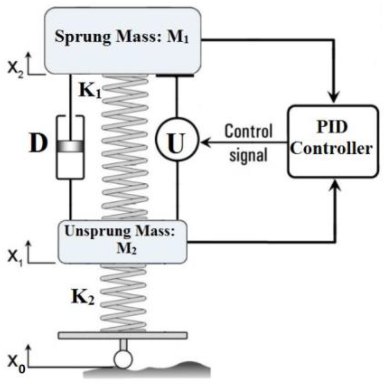
Figure 4.
Proposed quarter car model with PID controller.
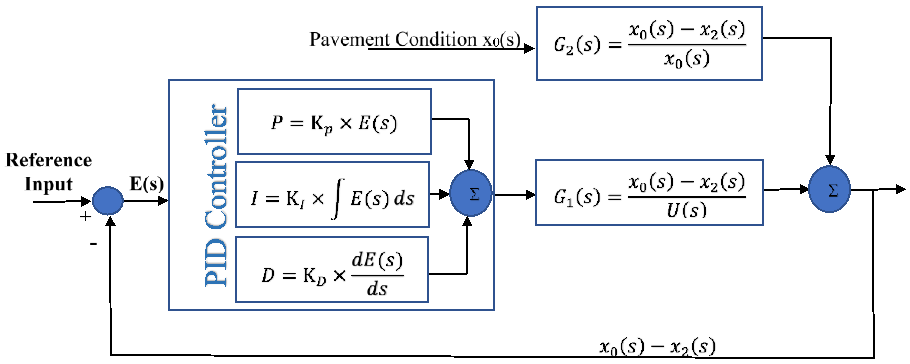
Figure 5.
MATLAB-Simulink model of the proposed fuel consumption and noise cancellation system for the active suspension system.
Figure 5.
MATLAB-Simulink model of the proposed fuel consumption and noise cancellation system for the active suspension system.

Figure 6.
Uncontrolled total system response, based on the random input.
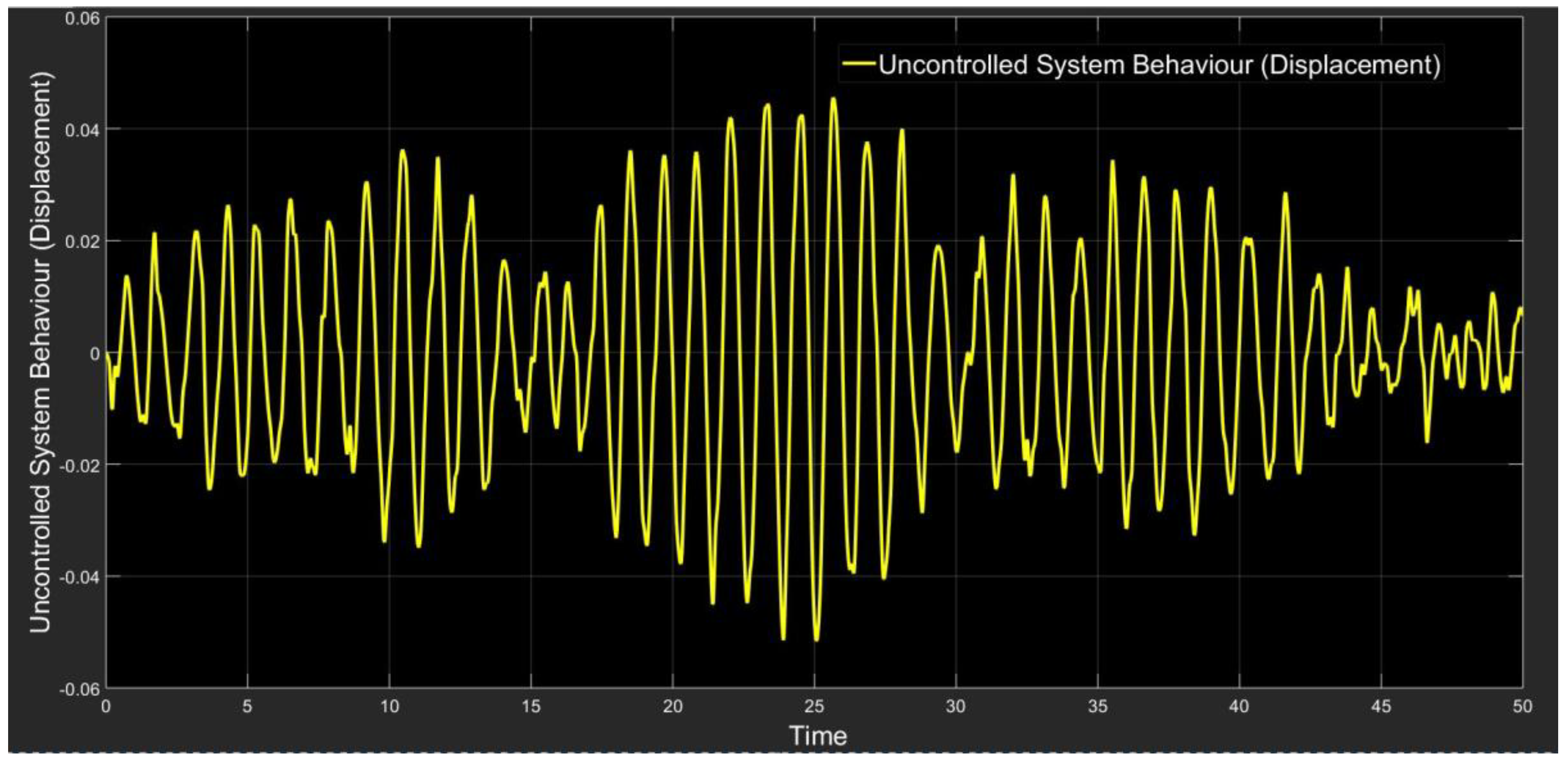
Figure 7.
Controlled total system response, based on the random input.
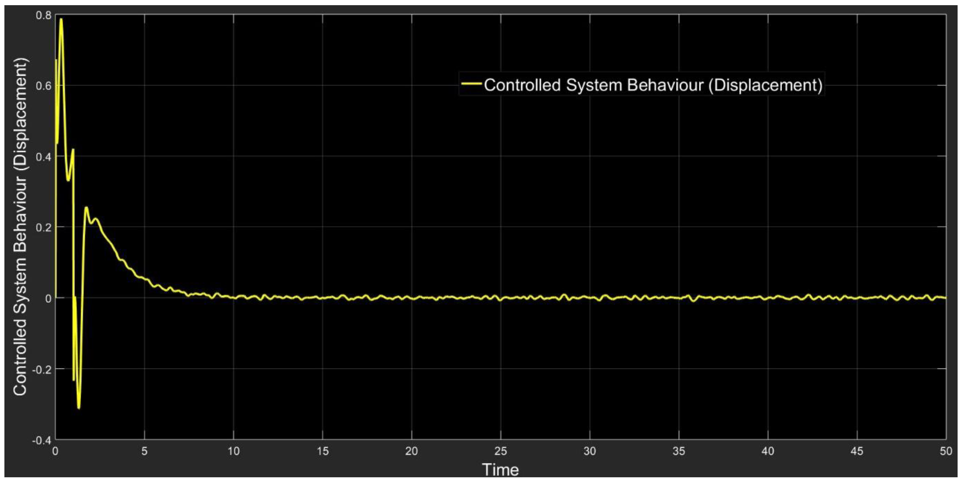
Figure 8.
Controlled and uncontrolled total system behaviors.

Figure 9.
Uncontrolled fuel consumption rate changes.

Figure 10.
Controlled change of the fuel consumption rate.
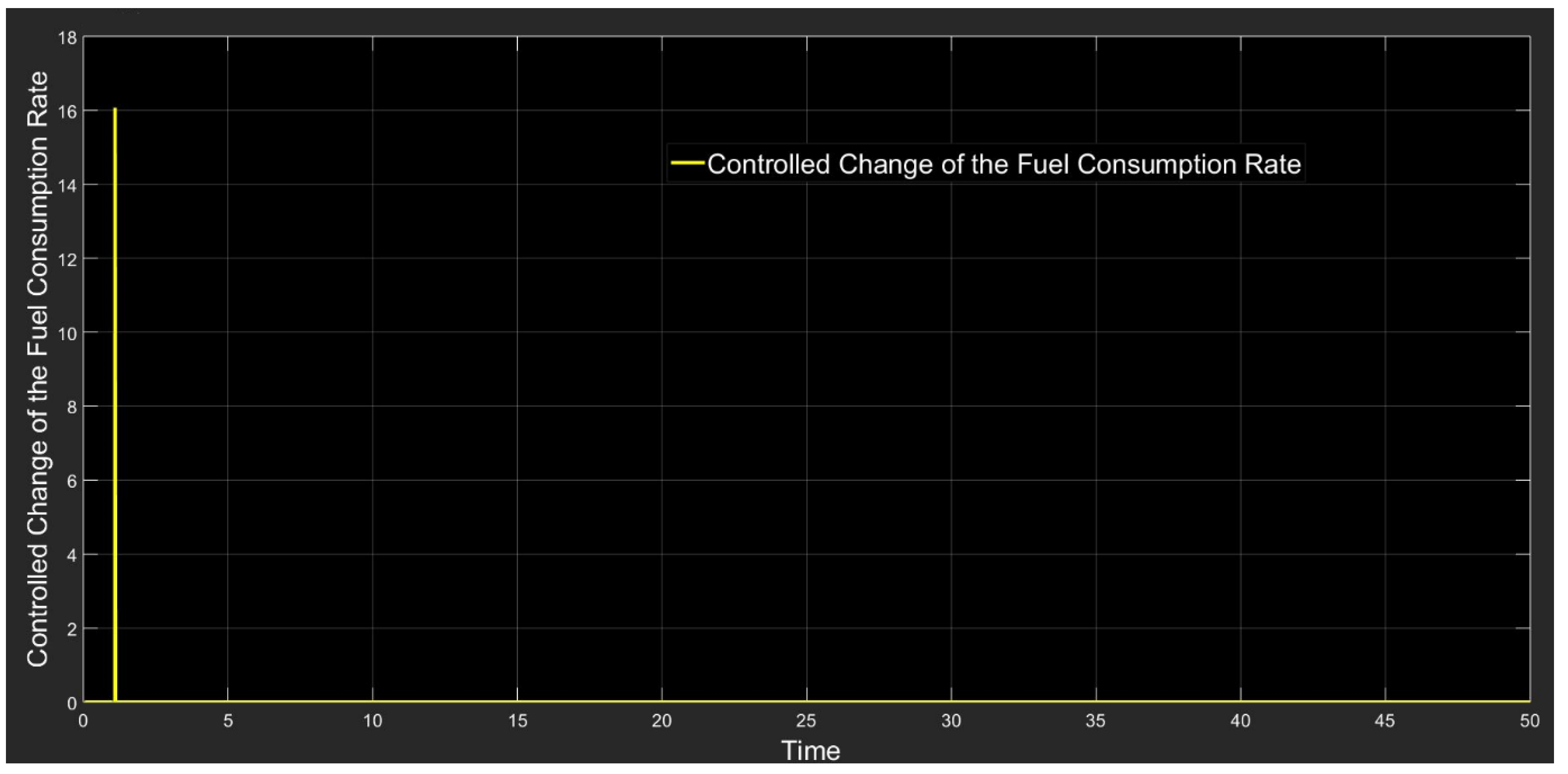
Figure 11.
Pole and zero information of the design PID controller.
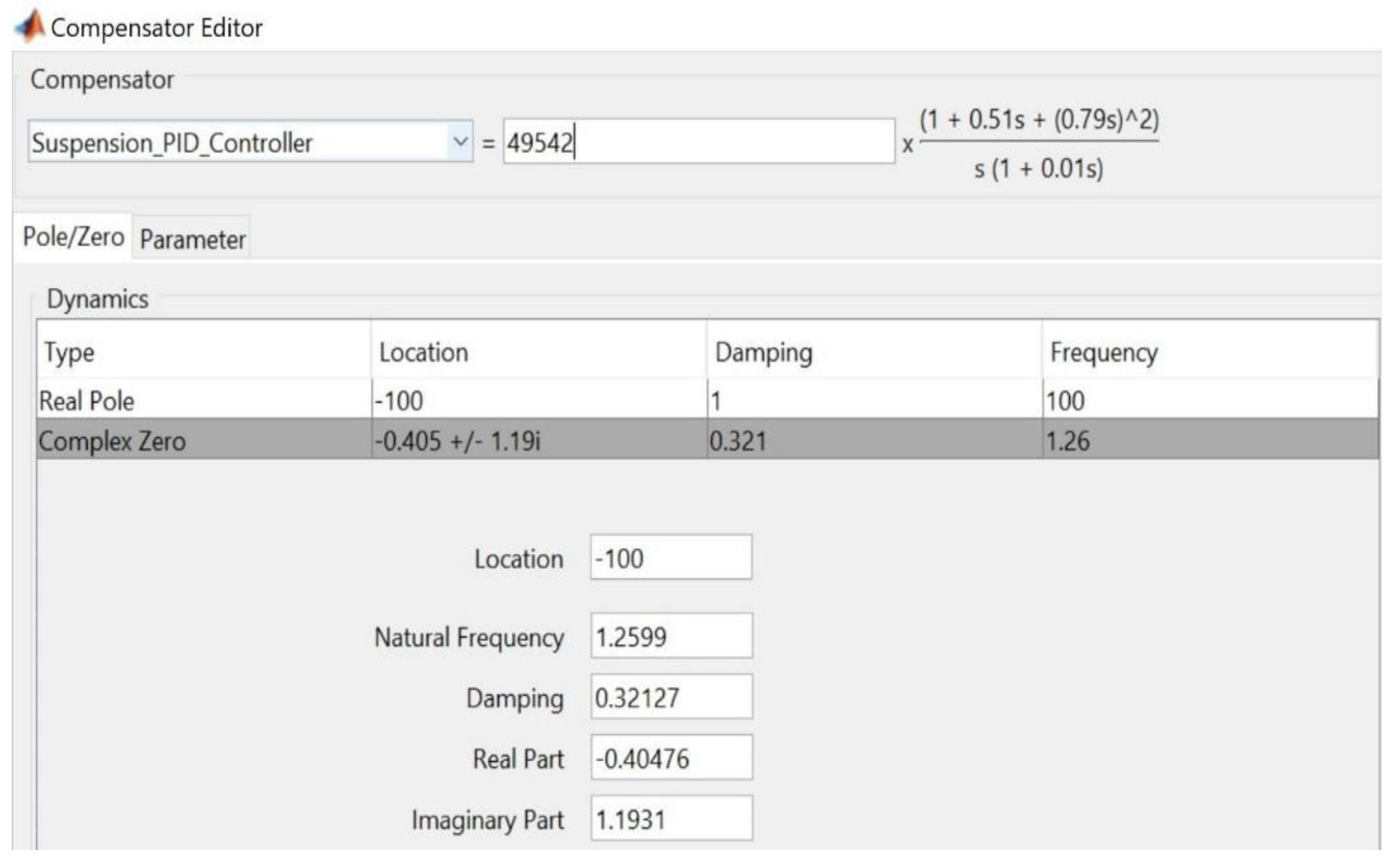
Figure 12.
Root locus diagram.


Table 1.
Response of PID controller.
| Parameter | Stability | Steady State Error | Settling Time | Overshoot | Rise Time |
|---|---|---|---|---|---|
 KP KP | Degrade | Decrease | Small Change | Increase | Decrease |
| KI | Degrade | Eliminate | Increase | Increase | Decrease |
| KD | Improve For small KD | No effect in theory | Decrease | Decrease | Minor Change |
Table 2.
Simulation parameters.
| Vehicle Model Parameters | Symbol | Numerical Value | Unit |
|---|---|---|---|
| Sprung Mass | M1 | 300 | kg |
| Unsprung Mass | M2 | 40 | kg |
| Suspension Stiffness | K1 | 15,000 | N/m |
| Tire Stiffness | K2 | 150,000 | N/m |
| Suspension Damping Coefficient | D | 1000 | Ns/m |
© 2018 by the author. Licensee MDPI, Basel, Switzerland. This article is an open access article distributed under the terms and conditions of the Creative Commons Attribution (CC BY) license (http://creativecommons.org/licenses/by/4.0/).
Share and Cite
MDPI and ACS Style
Azizi, A. Computer-Based Analysis of the Stochastic Stability of Mechanical Structures Driven by White and Colored Noise. Sustainability 2018, 10, 3419. https://doi.org/10.3390/su10103419
AMA Style
Azizi A. Computer-Based Analysis of the Stochastic Stability of Mechanical Structures Driven by White and Colored Noise. Sustainability. 2018; 10(10):3419. https://doi.org/10.3390/su10103419
Chicago/Turabian StyleAzizi, Aydin. 2018. "Computer-Based Analysis of the Stochastic Stability of Mechanical Structures Driven by White and Colored Noise" Sustainability 10, no. 10: 3419. https://doi.org/10.3390/su10103419
Note that from the first issue of 2016, this journal uses article numbers instead of page numbers. See further details here.