Sustainability of the Reanalysis Databases in Predicting the Wind and Wave Power along the European Coasts

Abstract

In the present work, the wind and wave conditions in the European nearshore are assessed considering a total of 118 years of data, covering the time interval from 1900 to 2017. In this context, special attention has been given to the western European coasts that are facing the ocean. In order to do this, the reanalysis data coming from three state-of-the-art databases (ERA Interim, ERA20C, and NCEP) were processed. Furthermore, a more complete picture was provided by also including the satellite measurements coming from the AVISO (Archiving, Validation and Interpretation of Satellite Oceanographic Data) project in the analysis. From this perspective, the distribution of the two marine energy resources was discussed, which throughout energetic maps—and further, on some specific reference sites—were defined at a distance of 50 km from the shore for more detailed analysis and comparison. As expected, the places located in the vicinity of the United Kingdom present more important energy resources, but some other interesting sites were also highlighted. Furthermore, although each dataset is defined by particular features, there is a similar pattern in the identification of the sites’ attractiveness, regardless of the database considered for assessment.

1. Introduction

On a European scale, a lot of effort has been made during the recent decades to promote the use of renewable sources in the energy market [1,2,3]. It is estimated that during the interval 2005–2014, the share of the renewable electricity sector was around 7% per year, compared with the renewable heating and cooling sectors, where only a 3% share was registered. These values are promising, particularly if we take into account that until 2020 an average annual growth of only 6% was predicted for the first sources, and 4% for the second ones, respectively. Up until the year 2015, almost 27% of the European Union’s reported electricity share was coming from renewables, with theexpectation that according to an optimal scenario, this percentage will increase to 50% by 2030 [4].

Most of these results are reported for the renewable sources that are located on the land, but gradually, the attention has shifted to the marine environment, where a wider range of natural resources can be found [5,6,7,8,9,10]. The European coastal regions play an important role, particularly if we take into account that almost 43% of the total population lives in these areas, and almost 38% of the inhabitants are concentrated in one of the 194 major cities (100,000 inhabitants) located at a maximum distance of 50 km from the sea, according to the values reported in 2007 [11].

On the other hand, it is difficult to assess the marine conditions from a large area throughout conventional in situ methods such as buoys, weather balloons, or ship observations, since these are restricted to a particular site and time window, and thus cannot possibly provide a complete picture of the spatial distribution of the natural resources [12,13]. In order to solve this problem, new techniques were developed in recent years. These are capable of accurately identifying the evolution of the wind and wave conditions, among which the satellite measurements can be mentioned [14], or the reanalysis databases [15]. There is a common practice among the scientific community to use synthetic databases or numerical simulations in order to assess these environmental conditions.

Sempreviva et al. [16] presented a complete description of the methodologies and databases used to evaluate the European offshore wind resources; however, this study was limited to the year 2008. The offshore wind conditions may be also evaluated throughout the satellite missions; this topic was covered in Hassager et al. [17], where the time interval from 1999 to 2012 was considered for investigation. In that work, special attention was given to the wind resources reported in the vicinity of some operational wind farms. From the enclosed European basins, the Mediterranean Sea seems to reveal the best wind and wave energy resources; this aspect has been highlighted by several scientific publications [18,19,20,21,22,23]. Soukissian and Papadopoulos [24] carried out a study where they investigated the effect of different wind data sources, such as in situ measurements, as well model generated and satellite observations, in order to assess the offshore resources in the eastern part of the Mediterranean Sea. As they mentioned, the long-term wind data provided by the reanalysis databases or the satellite measurements may be defined by various degrees of uncertainties. In recent years, the wind conditions from other enclosed seas, such as the Black Sea, havealso been considered for investigation [25,26,27] by using various data sources; the more promising results were those that reported on the wind power on the western part of these basins. As for the wave energy, there is interest in highlighting the performance of the wave energy converters [28,29,30,31,32]. Therefore, it is important to use a reliable dataset, such as the one provided by the European Center for Medium-Range Weather Forecast (ECMWF). The evolution of the wave characteristics over large water areas is identified by using numerical models that are focused on a global scale or adjusted for particular coastal environments [33,34,35].

In the work presented by Bernardino and Guedes Soares [36], the wind and waves from the Portuguese coast were evaluated from a meteorological point of view, by using the ERA Interim and ERA20C datasets. In this case, the analysis was limited to a single reference site, which was located approximately 260 km from the shore, for which a total of 110-years of data were processed. In Kalogeri et al. [37], a complete assessment of the European wind and wave conditions was carried out by taking into account the intermittency and variability of these resources. Although this work was published in 2017, the dataset considered for evaluation covers only the time interval from 2001 to 2010. A complete assessment of the wave energy from the vicinity of the Atlantic European coast was carried out by GuedesSoares et al. [38]; in this work, the wind fields from the ERA Interim database were used to force two spectral models. Although several wind fields were considered for investigation in this work, in general, these results are reported for a short time interval, which does not exceed four years. The wave energy potential from the Bay of Biscay was discussed in Iglesias and Carballo [39] by using a total of 44years of measurements and hindcast data (1958–2001), which indicate that more important resources seems to be reported on the eastern sector of this area.

After taking into account previous studies, the core of this work is structured around the following research questions and innovations:

• Highlighting the joint evaluation of the European wind and wave energy potential, by considering multiple datasets which cover the time interval from 1900 to 2017 (118 years of data in total);
• Identify the strong points and weak points of these datasets, in order to analyze their usefulness for meteorological or renewable energy studies;
• Highlight the spatial and seasonal agreement (if any), by considering various reference sites defined at about 50 km distance from the shoreline.

2. Materials and Methods

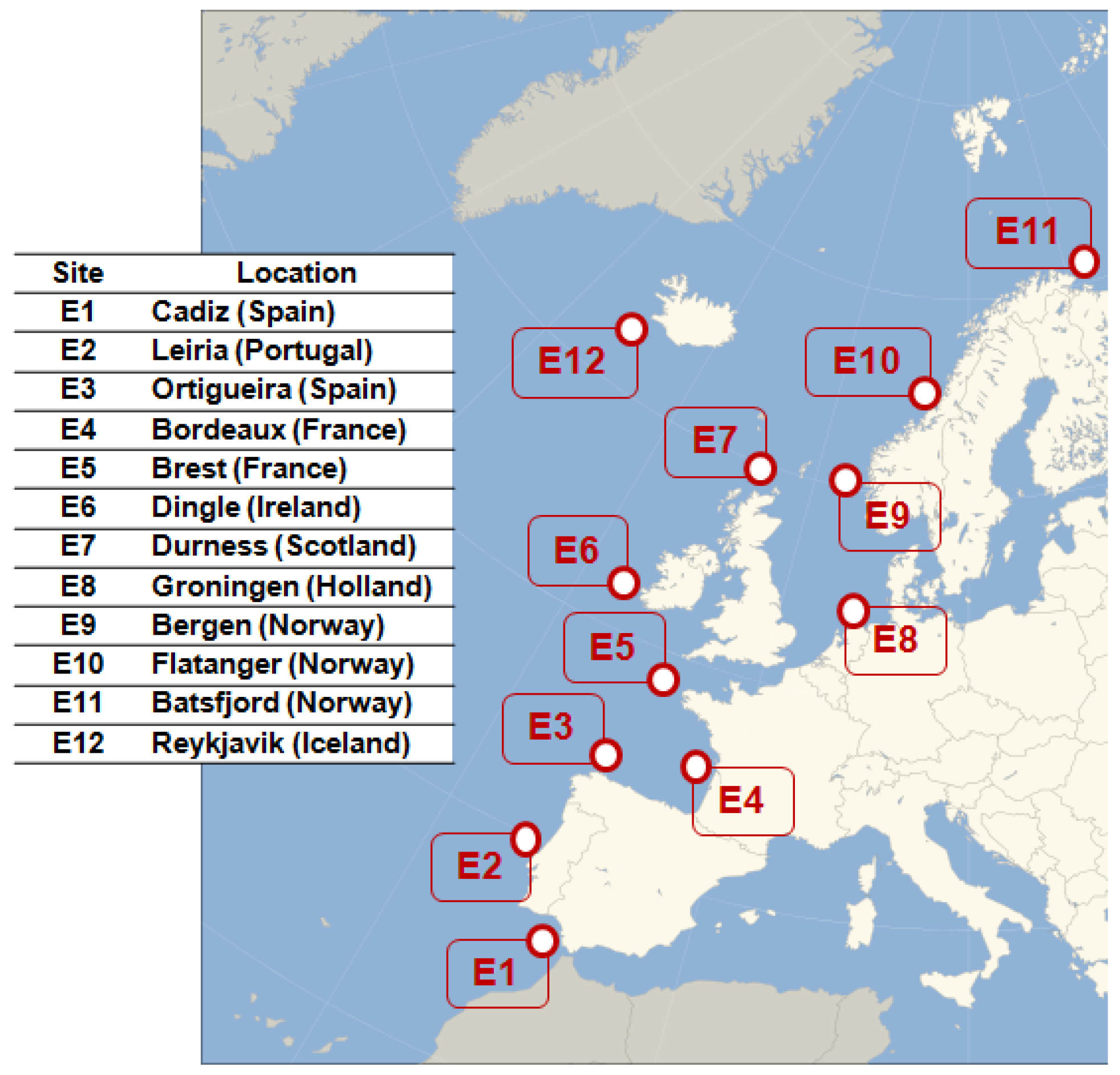
2.1. The Target Areas

Figure 1 illustrates a map of Europe that presents the 12 reference sites considered for evaluation, which are denoted from E1 to E12. These sites were defined at approximately 50 km from the shoreline, since it is possible in this way to identify the best marine conditions while also avoiding the missing values that may be reported by the satellite missions in the vicinity of the coastline [40]. All of the points are located on the western coast, being shared by: Spain—E1 (water depth = 436 m) and E3 (665 m); Portugal—E2 (348 m); France—E4 (92 m) and E5 (112 m); Ireland—E6 (123 m); Scotland—E7 (95 m); Holland—E8 (31 m); Norway—E9 (294 m), E10 (293 m) and E11 (321 m); Iceland—E12 (79 m). For each site, the most appropriate land site, which defines its geographical position, was also indicated.

2.2. Data

In this work, all of the data (wind and wave) coming from the reanalysis projects were extracted and processed on a European scale by using the NetCDF files associated to each project. In the case of the satellite measurements, the time series reported for each site were directly extracted from the associated user interface web page.

The first dataset considered for evaluation was ERA Interim, which comes from the European Center for Medium-Range Weather Forecasts (ECMWF); the data covers the interval from 1979 to the present. This is based on a high-resolution atmospheric model that is capable of incorporating in situ and satellite measurements throughout an assimilation system. Since 2006, this model uses an Integrated Forecast System (IFS) defined by 60 levels in the vertical and a Gaussian grid with uniform 79 km spacing between the points of the grid. The atmospheric model is linked to an ocean-wave model, which provides various wave characteristics on a global scale, by processing 24 wave directions and 30 wave frequencies [41,42,43]. The wind conditions are reported at a 10-m height above the sea level, being provided in terms of the U and V components. Nevertheless, since one objective of the present work is to assess the wind conditions from a renewable energy perspective, the initial conditions (at 10 m) will be adjusted to an 80 m level, which represents in general the lowest value at which an offshore wind turbine may operate. In this case, the following equation will be used [44]:

$$U_{80}=U_{10}\cdot \frac{\ln (z_{80})-\ln (z_{10})}{\ln (z_{10})-\ln (z_0)}$$

(1)

where: $U_{80}$—wind speed at 80 m (in m/s); and $U_{10}$—wind speed at 10 m (in m/s); while $z_{80}$ and $z_{10}$—the reference heights, which are 80 m and 10 m, respectively; and $z_0$—the roughness of the sea surface (0.01 m).

Another important parameter that will be considered in this work is the wind power (P_wind in W/m²), which is defined as [44]:

$$P_{wind}=\frac{\rho \cdot U_{80}^3}{2}$$

(2)

where: $\rho$—air density (≈1.22 kg/m³).

The second database is ERA20C, which is also a reanalysis product maintained by ECMWF, with the mention that this is part of the European Reanalysis of Global Climate Observations (ERA-CLIM) project. Although the dataset covers the entire 20th century (the interval from 1900 to 2010), this is relatively a young project that was produced in 2014 in about six weeks. The IFS model uses 91 vertical levels divided between the surface and a 89-km altitude, while the horizontal resolution of the grid is 125 km. There are two types of data assimilated in the project, namely: (a) surface and mean sea level pressure coming from the projects ISPDv3.2.6 and ICOADSv2.5.1; and (b) surface marine wind coming from the project ICOADSv2.5.1. The ocean waves are computed in this case by considering 25 frequencies and only 12 directions, among the parameters provided are the significant wave height (H_s), mean wave period (T_e) and wave direction [36,45].

Since most of the reference sites are located in deep water areas, the wave power (P_wave—kW/m), is evaluated throughout the equation [46]:

$$P_{wave}=\frac{\rho \cdot g^2}{64\cdot \pi }\cdot T_e\cdot H_s^2$$

(3)

where: $\rho$—seawater density (1025 kg/m³); and $g$—gravitational acceleration (9.81 m/s²).

Another dataset is related to the National Centers for Environmental Prediction (NCEP)–Climate Forecast System Reanalysis (CFSR), which will be denoted here with NCEP. It was developed around two main systems, namely CFSv1 and CFSv2, with the latest one considered an improved version. The first version was implemented in August 2004, and it was the first quasi-global, fully coupled atmosphere–ocean–land model capable of predicting the seasonal distribution at the NCEP center. Various sources of observations are included in this project, among which can be mentioned the special sensor microwave/imager (SSM/I) reported by the DMSP (Defense Meteorological Satellite Program) satellites, or the satellite missions from the European Space Agency. Similar to the wind conditions reported by the ERA-Interim and ERA20C, the wind values included in the NCEP data are reported at a 10-m height [47,48].

The last database considered in this work is related to the altimeter wind and wave measurements distributed by AVISO, which collect and assemble data from multiple missions. The satellite altimeter estimates the H_s parameter along the satellite track by measuring the slope of the return pulse, which is indicated by the delay reflection of the beam between the wave trough and crest. They also reveal the wind conditions by evaluating the radar cross-section, which depends on the roughness of the sea surface measured at different incident angles. From the satellite mission used in the AVISO project, ERS1, ERS2, and TOPEX/Poseidon can be mentioned, which can measure the 10-m wind vector for a radar cross-section of 500 km [49,50].

Table 1. Summary of the datasets considered for evaluation. NCEP: National Centers for Environmental Prediction. ERA: European Reanalysis.

Database →	ERA Interim	ERA20C	NCEP	AVISO
Characteristic↓
Parameter	wind/waves	wind/waves	wind	wind/waves
Start date	1979-01-01	1900-01-01	1979-01-01	2009-09-14
End date	2017-07-31	2010-12-31	2010-12-31	2017-11-26
Time step	6 h (4 per day)	6 h (4 per day)	1 h (24 per day)	1 per day
Spatial resolution (°)	0.75°× 0.75°	0.75°× 0.75°	0.312°× 0.312°	1°× 1°

presents the four datasets processed for this study, from which three represent reanalysis products (ERA-Interim, ERA20C, and NCEP), and the last one is associated with the satellite measurements coming from the AVISO project. Each database is defined by various characteristics, such as the spatial and temporal resolution, and the availability of different time periods. In 2010, the ERA20C and NCEP projects were stopped, while the rest of the databases are still operational. Except for the NCEP database, all of the other projects provide data related to the wind and wave conditions, with the mention that in the case of the AVISO measurements, the wave period and wave direction were not available.

By screening the reanalysis databases, it was noticed that there are no missing data, but in the case of the AVISO measurements, this situation is encountered, as we can see in Figure 2. The results are reported for the total (full time distribution) and winter time (interval from October to March), while a dotted line represented the 10% limit [51].

It is considered that the accuracy of the results significantly decreases if the percentage of the missing values exceeds this limit. In general, it can be observed that most of the values are located below this limit, with the exception of site E11 (Norway), which reveals a maximum of 71.3% for the wind and 21% for the wave conditions. In this case, the technique proposed in Makarynskyy et al. [52] can be also considered to fill the gaps.

Regarding this aspect, it was noticed that for the wind conditions encountered during the interval 8.04.2012 and 26.11.2017, only NaN (Not a Number) were reported, while for the waves, a similar situation was encountered for the interval 8.04.2012 and 3.09.2013. In this case, the reference site E11 will not be further considered for investigation when the AVISO data is evaluated.

In the case of the wind data, sites E1, E2, E4, and E5 present maximum missing data values located in the range of 8.3% and 16%, which means that the accuracy of the results reported for sites E1 and E4 may be influenced. As for the wave values, site E4 presents a maximum of 7.6%, while sites E3, E7, E9, E10, and E12do not have any missing data noticed; this aspect is also reflected in the case of the wind conditions.

3. Analysis of the Wind and Wave Conditions

Figure 3 presents the spatial distribution of the wind resources by taking into account the average values (at 80 m) as reflected by the ERA Interim database. It can be observed that more consistent values are accounted by the offshore areas located in the North Atlantic Ocean, where a maximum wind power of 1600 W/m² may be considered representative for the interval 1979 and 2017. From an energetic point of view, the western coast of Ireland and Scotland seems to reveal the best wind conditions, which is also the case for the southern part of Iceland.

The southwestern part of Norway and the sites located in the North Sea may have a wind power located in the range of 1000 W/m² and 1500 W/m²; these values are also encountered in the Celtic Sea. From the Iberian peninsula, the best resources seem to be reported close to the Galicia region (Spain), where a maximum peak of 800 W/m² is noticed, with the mention that in the vicinity of the coastline, the wind power does not exceed 500 W/m². As for the enclosed seas, the Baltic Sea seems to have the best resources (≈600 W/m²), followed by the Mediterranean Sea and the Black Sea. It is important to mention that for the last two basins, some hotspots are noticed in the area. The first one is located in the northwestern part of the Mediterranean Sea close to Gulf of Lion, while for the same basin, the sites from the Aegean Sea seems to present a similar pattern. The western part of the Black Sea and the region located in the east of Crimean peninsula present more consistent wind resources. In some of these cases, the general wind pattern is influenced by the local conditions, such as the occurrence of the Bora events [25].

A similar evaluation is presented in Figure 4; this time, the wave power is assessed, which presents a maximum value of 78.7 kW/m in the offshore area, more precisely, the region located between the United Kingdom (UK) and Iceland. As the waves approach the shore, the level of energy is gradually attenuated, with reported values of 65 kW/m in the vicinity of Ireland and Scotland, and close to 50 kW/m in some parts of Norway and in the north of the Iberian peninsula. In general, the wind and waves go hand in hand, and therefore, the sites with good wind resources are also defined by consistent wave resources. The enclosed basins are defined by much lower resources (below 15 kW/m), which seems to be more important in some areas in the Mediterranean Sea, and in the southern part of the Baltic Sea.

Figure 5 illustrates the distribution of the wind and wave resources (average values) reported by the ERA20C dataset for all of the 12 reference sites considered for evaluation (E1–E12). The results are structured in total and winter time, and as it can be observed, the values reported during the winter season are more energetic. In terms of wind energy (Figure 5a), site E6 (Ireland) seems to be more energetic, with a maximum of 1414 W/m² in the winter, and 1027 W/m² for the total time.

Sites E3, E5, E7, E11, and E12 also reveal important values, which may reach a maximum of 1170 W/m² (during winter), while the remaining sites have values that are located below 507 W/m². From this point of view, much lower values correspond to sites E1 and E2, which are located in the vicinity of the Iberian coasts.

Regarding the waves (Figure 5b), site E6 also revealed the maximum values (60.35 kW/m), followed by E3, with 45.6 kW/m. Except for sites E1 and E8, which account for the lowest values (below 10.3 kW/m), the rest of the sites seems to be on the same level, with values varying between 17.4 kW/m during the total time and 28 kW/m in winter, respectively.

A complete description of the two marine conditions can be carried out by taking into account the annual, seasonal, and monthly variability indexes (AV, SV, and MV, respectively), which indicate the degree of energy fluctuations for various time intervals. They are defined as the differences between the most energetic value and the least energetic one, which are divided at an average value, as it can be observed from the following equations [53]:

$$AV=\frac{P_{A\max }-P_{A\min }}{P_{year}};SV=\frac{P_{S\max }-P_{S\min }}{P_{season}};MV=\frac{P_{M\max }-P_{M\min }}{P_{month}}$$

(4)

For example, in the case of the AV index, there were 111 maximum and 111 minimum values identified (for each year), from which the absolute maximum (and minimum values) were selected in order to define the parameters P_Amax and P_Amin, respectively. At the end, this index represented by a single value was obtained by dividing the difference (max−min) to an average annual value (P_year) reported for each site. In the case of the seasonal index (SV), it was considered to be the difference reported between the winter season (interval from October to March) and the remaining time interval (from April to September), which will be further denoted as summer. In a similar way, the differences reported between the two absolute seasonal values (max–min) will be divided to arrive at an average value. As for the MV index, there were 12 maximum and 12 minimum values corresponding to each month computed, from which only the absolute values (maxim and minimum) were considered. Although the average values (P_year, P_season, and P_month) are denoted in a different way for each index, in fact they are identical, since the average value that is evaluated corresponds to the entire dataset regardless of the year, season, or month.

The evolution of these synthetic indexes is illustrated in Figure 6. As it can be observed, the wave energy fluctuation is more significant than in the case of the wind, while the monthly variability seems to present much higher values, regardless of the parameters that are taken into account.

For the wind energy, the AV index in general has values in the range of 0.63 and 1, which is much lower than the values being indicated for sites E2 and E11, respectively. In terms of the seasonal variability (reported between winter and summer), a minimum of 0.28 is reported close to site E2, while the maximum values do not exceed 0.88 (site E10). For the monthly variations, the values oscillate around the value 1.2, with a reported minimum of 0.66 close to E2 (Portugal), while a higher variation may be noticed close to E11 (Norway).

As for the wave energy, the SV and MV indexes have in general constant values (1.15 and 1.85, respectively), with the mention that a maximum peak of 0.95 and 1.42 are noticed for site E8. The annual values gradually increase from site E2 (0.8) until they reach site E10 (1.22), and after this maximum, the variability tends to be reduced until they reach a value of 0.91, close to E12.

The wind conditions coming from the NCEP project were also evaluated, considering the time interval from 1979 to the end of 2010. Figure 7 illustrates the distribution of the wind power (average values) reported for a height of 80m. In this case, site E6 is indicated as being more energetic, with a wind power of 1832 W/m² during the winter, and 1308 W/m² for the total time, while on the opposite side, site E1 does not exceed 56 W/m². The value reported by site E6 during the total time exceeds most of the values reported during the winter, with the exception of sites E11 and E12, which during this season presented a maximum of 1396 W/m² and 1536 W/m², respectively.

Compared with some other reanalysis databases (such as ERA Interim and ERA20C), which provide only four values per day (00-06-12-18 UTC), the NCEP dataset is defined by an hourly resolution, which allows the evaluation of the wind power fluctuation on a more detailed scale. Figure 8 illustrates such a distribution by taking into account all of the reference sites thatpresent some particular hourly patterns. Sites E1 and E2 are dominated by some energetic peaks of 54.52 W/m² (at 15 UTC (Universal Time Coordinated)) and 388 W/m² (at 17 UTC), with a similar pattern noticed for E7 and E8, with a maximum of 760 W/m² (between 12–14 UTC) and 628.4 W/m² (at 13 UTC), respectively. Site E10 presents several fluctuations during the day. Meanwhile, for site E12, more important wind resources are noticed during the nocturnal interval, especially after the 20 UTC, when a maximum of 1119 W/m² may be reported. For site E11, the wind power values varied between 1000–1041 W/m², with the mention that the values corresponding to the interval 7 UTC and 18 UTC tend to be higher. For sites E3, E5, and E6, the results indicated for 1 UTC indicate the lowest values, which are quickly moved to higher values as they approach 2 UTC. In addition to this, site E6 also presents two minimum peaks (for 13 UTC and 19 UTC), the first one being also reported by site E4, while the last one is visible in the case of site E9.

The wind resources (at 80 m) indicated by the AVISO satellite measurements are represented in Figure 9. From this distribution, it can be observed that the group sites E1–E5 present lower values, compared with the remaining sites, with the mention that site E11 was not considered for evaluation. In this case, sites E6 and E7 seem to present the best wind resources, with a maximum of 984 W/m², with the mention that this time, site E7 appears to be more energetic. Other relevant sites are E9 and E12, while site E1 is on the opposite side, with a minimum value of 176 W/m² (total time) and 219 W/m² (in winter). From the group sites E1–E5, sites E3 (Spain) and E5 (France) present more consistent values, which may reach a maximum of 560 W/m² during the winter season.

4. Discussion of the Results

A statistical analysis of the wind energy corresponding to all of the databases considered (ERA Interim, ERA20C, NCEP, and AVISO) is provided in

Table 2. Wind power density (P_wind—in W/m²) reported at a height of 80 m above sea level, corresponding to the total time distribution.

Sites→		E1	E2	E3	E4	E5	E6	E7	E8	E9	E10	E11	E12
Database↓
ERAInterim(1979–2017)	Mean	196	270	810	277	754	1177	1066	453	435	560	817	945
	95th	775	943	2992	1156	2802	4184	3860	1704	1803	2327	2930	3542
	99th	1570	1694	5286	2534	5082	7180	6676	3028	3394	4643	4928	6357
ERA20C(1900–2010)	Mean	183	176	689	281	674	1026	766	376	321	350	763	831
	95th	703	637	2619	1171	2579	3660	2802	1395	1259	1456	2797	3096
	99th	1556	1219	4718	2506	4592	6212	4735	2444	2262	2892	4853	5443
NCEP(1979–2010)	Mean	41	290	851	384	841	1308	725	573	627	570	1022	1078
	95th	164	1080	3158	1520	3152	4729	2875	2186	2632	2362	3689	4180
	99th	373	1956	5863	3136	5803	8604	5440	3934	5235	4784	6519	8302
AVISO(2009–2017)	Mean	176	300	382	256	376	667	661	433	578	507	x	627
	95th	696	1256	1525	1148	1624	2663	2636	1620	2349	2194	x	2423
	99th	1438	2445	3103	2379	2990	4851	4507	3485	4051	3764	x	3923

. This was made by evaluating the parameters: mean value, 95^th percentile (denoted as 95^th), and 99^th percentile (99^th), respectively. The mean values were already discussed in the previous section, and although the results are reported for different time intervals, some common patterns seem to occur. Obviously, there is a strong connection between the wind power and the wind speed (Equation (2)), where the amount of energy varies with the cube (the third power) of the wind speed. For example, if the wind speed doubles, the power will increase eight times, while if the speed quadruples, the wind power will increase 64 times. Therefore, the presence of higher/extreme wind values in a dataset may significantly influence the accuracy of the results, as it can be observed in the case of site E6, which presents the highest percentile values. For this site, the 95^th percentile has the following values: ERAInterim—4184 W/m²; ERA20C—3660 W/m²; NCEP—4729 W/m²; and AVISO—2663 W/m², the differences being much higher in the case of the 99^th index, where a maximum of 8604 W/m² is noticed by the NCEP database.

In the case of site E1, which seems to be characterized by moderate wind resources, the NCEP data present a minimum of 373 W/m² for the 99^th, compared with a value located close to 1500 W/m², which is reported by the ERAInterim, ERA20C, and AVISO, respectively. Although different time intervals were considered for investigation, it seems that the NCEP dataset under evaluates the wind resources from the southern extremity of Europe, which is not the case for the other sites, such as E2 and E3, where the values are significantly higher than the rest of the considered databases. In some cases (ex: site E6 and E12), the 99^th reported by the NCEP is double the values reported by the AVISO measurements. The higher values reported by the NCEP data may be related to the NCEP data being defined by 24 values per day, compared with four in the case of the ECMWF projects, and one measurement for AVISO. It is possible that the wind power density reported for this dataset is more sensitive to the occurrence of the lower or extreme wind values, especially if we consider extrapolating the dataset to a particular wind turbine hub. The variations reported between the reanalysis datasets may be also linked to the presence/absence of the in situ measurements (in the assimilation process) from a particular geographical area, which may significantly influence the output of the numerical simulations.

Throughout the normalized values, it is possible to rank the sites according to their energy attractiveness by dividing the wind power of each site by the maximum value of all of the sites considered. A similar analysis is presented in Figure 10, where the maximum wind power for each wind database was also indicated, which in this case corresponds to site E6. On the top of the four most promising sites we found: E6 (Ireland), E7 (Scotland), E12 (Iceland), and E11 (Norway) as indicated by both the ERA Interim and ERA20C. As regards the NCEP data, site E7 is replaced with E3 (Spain), while in the case of AVISO, site E12 is replaced by E9 (Norway). On the other hand, lower wind resources seem to be representative for sites E1 (Spain), E2 (Portugal), and E4 (France).

A detailed assessment of the wave resources is presented in

Table 3. H_s statistics corresponding to the total time.

Sites→		E1	E2	E3	E4	E5	E6	E7	E8	E9	E10	E11	E12
Database↓
ERAInterim(Hs→m)	Mean	0.82	1.31	2.53	1.54	2.17	3.05	1.56	0.62	1.65	2.10	2.01	2.36
	95th	1.58	2.50	5.04	3.31	4.52	6.17	3.23	1.38	3.42	4.47	4.11	4.89
	99th	2.21	2.26	6.75	4.54	6.14	8.26	4.32	1.87	4.45	6.05	5.51	6.60
ERA20C(Hs→m)	Mean	0.78	1.54	2.21	1.41	1.93	2.54	1.83	1.24	1.72	1.72	1.77	1.96
	95th	1.63	3.13	4.57	3.17	4.17	5.27	3.78	2.93	3.78	3.90	3.88	4.24
	99th	2.32	4.23	6.17	4.48	5.71	7.04	5.05	4.09	5.18	5.51	5.45	5.81
AVISO(Hs→m)	Mean	1.55	2.40	2.52	2.02	2.17	2.97	2.67	1.44	2.52	2.46	x	2.69
	95th	2.79	4.43	4.90	4.17	4.43	5.66	5.01	2.82	4.87	4.98	x	5.01
	99th	3.60	5.62	6.71	6.00	5.83	7.33	6.12	3.68	6.06	6.24	x	5.86

and Figure 11, where instead of the P_wave, the parameter H_s was evaluated in order to be able to also discuss the AVISO data. The H_s values reported by the AVISO are higher than the ones coming from the ECMWF project, indicating mean values in the range of 1.44–2.97 m. As for the normalied values, according to the ERA Interim and ERA20C, the most promising sites are E6, E3, E12, and E5, while in the case of AVISO, only sites E6 and E12 are included in top four. Sites E1 and E8 are indicated as being less attractive in terms of the wave resources, with the mention that site E1 also presents lower wind conditions.

5. Conclusions

As expected, the wind and wave energy characteristics are significantly influenced by different factors such as the combination of latitude and longitude, the distance from the shore, or the spatial orientation of the coastline. Most of the sites suitable for the marine renewable projects seem to be mainly located around the UK, but in the context of Brexit, it is expected that the European focus will be shifted to some other areas with relevant marine resources. According to a first estimation, it seems that the sites located between Portugal and the UK need to be moved farther in the offshore areas in order to become competitive with the sites from central or northern Europe from an energetic point of view. In some cases, it is possible to benefit from the presence of some “hot-spot” areas, where the marine resources are naturally concentrated, as in the case of the Galicia region (Spain) or the Gulf of Lion from the Mediterranean Sea. It is important to mention that Iceland presents excellent wind and wave resources, which in most of the cases exceed those from the coastal environment of the UK. Although the data coming from the three reanalysis projects (ERA Interim, ERA20C, and NCEP) and from the AVISO satellite were processed for different time intervals, it was noticed that the NCEP project indicated higher wind conditions compared with AVISO, which on the other hand indicates higher H_s values. The most promising sites in terms of the wind and wave energy are in general similar, regardless of the dataset considered for investigation; this was also the case for the sites defined by lower resources. It seems that the year 2010 represents a critical point for the reanalysis databases, during which some of them were stopped or replaced with more performing models.

Besides the energy potential, another important aspect of this research is related to the variability of these resources, which were highlighted throughout the wind and wave data reported by the ERA20C and NCEP databases, respectively. In general, the wave conditions presented higher variability, since the monthly variability is more significant compared with the annual variability, for example. As for the wind variability, it seems that some sites (ex: E1, E2, E7, and E8) follow a daily cycle, where during the interval 10 UTC and 19 UTC, they report more important wind resources.

It can be also underlined that the variation of the marine resources can be accurately identified for different time scales by using reanalysis databases or satellite measurements, but it is important to understand the limitations of these data in order for them to be useful for specific applications, such as maritime transportation, renewable energy, or coastal protection.

Finally, it has to be also highlighted that the work is still ongoing, and some other relevant datasets are going to be also analyzed in order to give a more complete picture of the convergence and differences that are existent between various data sources that provide the environmental conditions in the coastal areas. From this perspective, the next target would be to consider also NOAA WAVEWATCH IIICFSR Reanalysis Hindcasts [54].

References

1. Lendle, A.; Schaus, M. Sustainability Criteria in the EU Renewable Energy Directive: Consistent with WTo Rules? ICTSD Information Note No. 2; International Centre for Trade and Sustainable Development: San Francisco, CA, USA, 2010; ISSN 1994-6856. [Google Scholar]
2. Fabra, N.; Matthes, F.C.; Newbery, D.; Colombier, M. The Energy Transition in Europe: Initial Lessons from Germany, the UK and France; Towards a Low Carbon European Power Sector; CERRE (Centre on Regulation in Europe): Brussels, Belgium, 2015. [Google Scholar]
3. Deloitte, C. Energy Market Reform in Europe. European Energy and Climate Policies: Achievements and Challenges to 2020 and Beyond; Deloitte Conseil: Paris, France, 2015. [Google Scholar]
4. EEA (European Environment Agency). Renewable Energy in Europe 2017. Recent Growth and Knock-on Effects; EEA Report No. 3/2017; EEA: Copenhagen, Denmark, 2017; ISBN 978-92-9213-848-6. [Google Scholar]
5. Eurosion. Living with Coastal Erosion in Europe: Sediment and Space for Sustainability. Part IV—A guide to Coastal Erosion Management Practices in Europe: Lessons Learned; Service Contract B4—3301/2001/329175/MAR/B3; EUCC: Leiden, The Netherlands, 2004. [Google Scholar]
6. Randazzo, G.; Raventos, J.S.; Stefania, L. Coastal Erosion and Protection Policies in Europe: From EU Programme (Eurosion and Interreg Projects) to Local Management. In Coastal Hazards. Coastal Research Library; Finkl, C., Ed.; Springer: Dordrecht, The Netherlands, 2013; Volume 1000. [Google Scholar]
7. Onea, F.; Rusu, E. The expected efficiency and coastal impact of a hybrid energy farm operating in the Portuguese nearshore. Energy 2016, 97, 411–423. [Google Scholar] [CrossRef]
8. Rusu, E.; Onea, F. Study on the influence of the distance to shore for a wave energy farm operating in the central part of the Portuguese nearshore. Energy Convers. Manag. 2016, 114, 209–223. [Google Scholar] [CrossRef]
9. Diaconu, S.; Rusu, E. The environmental impact of a Wave Dragon array operating in the Black Sea. Sci. World J. 2013, 498013. [Google Scholar] [CrossRef] [PubMed]
10. Rusu, L.; Butunoiu, D.; Rusu, E. Analysis of the extreme storm events in the Black Sea considering the results of a ten-year wave hindcast. J. Environ. Prot. Ecol. 2014, 15, 445–454. [Google Scholar]
11. Collet, I. Portrait of EU Coastal Regions; Eurostat 38/2010; Eurostat Agriculture and Fisheries: Luxembourg, 2010; ISSN 1977-0316. [Google Scholar]
12. Souvorov, A.V. Marine Ecologonomics. The Ecology and Economics of Marine Natural Resources Management; Elsevier: Amsterdam, The Netherlands, 1999; ISSN 0-444-82659-9. [Google Scholar]
13. Xu, G.; Shen, W.; Wang, X. Applications of wireless sensor networks in marine environment monitoring: A survey. Sensors 2014, 14, 16932–16954. [Google Scholar] [CrossRef] [PubMed]
14. Krogstad, H.E.; Barstow, S.F. Satellite wave measurements for coastal engineering applications. Coast. Eng. 1999, 37, 283–307. [Google Scholar] [CrossRef]
15. Janssen, P.; Bidlot, J.-R.; Abdalla, S.; Hersbach, H. Progress in Ocean Wave Forecasting at ECMWF; European Centre for Medium-Range Weather Forecasts Report; ECMWF: Reading, UK, 2005. [Google Scholar]
16. Sempreviva, A.M.; Barthelmie, R.J.; Pryor, S.C. Review of methodologies for offshore wind resource assessment in European seas. Surv. Geophys. 2008, 29, 471–497. [Google Scholar] [CrossRef]
17. Hasager, C.B.; Mouche, A.; Badger, M.; Bingol, F.; Karagali, I.; Driesenaar, T.; Stoffelen, A.; Pena, A.; Longepe, N. Offshore wind climatology based on synergetic use of Envisat ASAR, ASCAT and QuikSCAT. Remote Sens. Environ. 2015, 156, 247–263. [Google Scholar] [CrossRef] [Green Version]
18. Emmanouil, G.; Galanis, G.; Kalogeri, C.; Zodiatis, G.; Kallos, G. 10-year high resolution study of wind, sea waves and wave energy assessment in the Greek offshore areas. Renew. Energy 2016, 90, 399–419. [Google Scholar] [CrossRef]
19. Foti, E.; Musumeci, R.; Leanza, S.; Cavallaro, L. Feasibility of an offshore wind farm in the gulf of Gela: Marine and structural issues. Wind Eng. 2010, 34, 65–84. [Google Scholar] [CrossRef]
20. Iuppa, C.; Cavallaro, L.; Foti, E.; Vicinanza, D. Potential wave energy production by different wave energy converters around Sicily. J. Renew. Sustain. Energy 2015, 7. [Google Scholar] [CrossRef]
21. Liberti, L.; Carillo, A.; Sannino, G. Wave energy resource assessment in the Mediterranean, the Italian perspective. Renew. Energy 2013, 50, 938–949. [Google Scholar] [CrossRef]
22. Omrani, H.; Drobinski, P.; Arsouze, T.; Bastin, S.; Lebeaupin-Brossier, C.; Mailler, S. Spatial and temporal variability of wind energy resource and production over the North Western Mediterranean Sea: Sensitivity to air-sea interactions. Renew. Energy 2017, 101, 680–689. [Google Scholar] [CrossRef]
23. Soukissian, T.; Karathanasi, F.; Axaopoulos, P. Satellite-based offshore wind resource assessment in the Mediterranean Sea. IEEE J. Ocean. Eng. 2017, 42, 73–86. [Google Scholar] [CrossRef]
24. Soukissian, T.H.; Papadopoulos, A. Effects of different wind data sources in offshore wind power assessment. Renew. Energy 2015, 77, 101–114. [Google Scholar] [CrossRef]
25. Onea, F.; Rusu, E. Wind energy assessments along the Black Sea basin. Meteorol. Appl. 2014, 21, 316–329. [Google Scholar] [CrossRef]
26. Onea, F.; Raileanu, A.; Rusu, E. Evaluation of the wind energy potential in the coastal environment of two enclosed seas. Adv. Meteorol. 2015, 2015, 808617. [Google Scholar] [CrossRef]
27. Onea, F.; Deleanu, L.; Rusu, L.; Georgescu, C. Evaluation of the wind energy potential along the Mediterranean Sea coasts. Energy Explor. Exploit. 2016, 34, 766–792. [Google Scholar] [CrossRef]
28. Liliana, R.; Onea, F. The performance of some state-of-the-art wave energy converters in locations with the worldwide highest wave power. Renew. Sustain. Energy Rev. 2017, 75, 1348–1362. [Google Scholar] [CrossRef]
29. Zanopol, A.T.; Onea, F.; Rusu, E. Evaluation of the coastal influence of a generic wave farm operating in the Romanian nearshore. J. Environ. Prot. Ecol. 2014, 15, 597–605. [Google Scholar]
30. Liliana, R.; Onea, F. Assessment of the performances of various wave energy converters along the European continental coasts. Energy 2015, 82, 889–904. [Google Scholar] [CrossRef]
31. Rusu, E. Evaluation of the wave energy conversion efficiency in various coastal environments. Energies 2014, 7, 4002–4018. [Google Scholar] [CrossRef]
32. Rusu, E.; Onea, F. Estimation of the wave energy conversion efficiency in the Atlantic Ocean close to the European islands. Renew. Energy 2016, 85, 687–703. [Google Scholar] [CrossRef]
33. Fan, Y.; Lin, S.-J.; Held, I.M.; Yu, Z.; Tolman, H.L. Global ocean surface wave simulation using a coupled atmosphere-wave model. J. Clim. 2012, 25, 6233–6252. [Google Scholar] [CrossRef]
34. Rusu, L.; Bernardino, M.; Soares, C.G. Wind and wave modelling in the Black Sea. J. Oper. Oceanogr. 2014, 7, 5–20. [Google Scholar] [CrossRef]
35. Rusu, L. Assessment of the wave energy in the Black Sea based on a 15-year hindcast with data assimilation. Energies 2015, 8, 10370–10388. [Google Scholar] [CrossRef]
36. Bernardino, M.; Guedes Soares, C. Evaluating marine climate change in the Portuguese coast during the 20th century. In Maritime Transportation and Harvesting of Sea Resources; Guedes Soares & Teixeira, Ed.; Taylor & Francis Group: London, UK, 2018; pp. 1089–1095. [Google Scholar]
37. Kalogeri, C.; Galanis, G.; Spyrou, C.; Diamantis, D.; Baladima, F.; Koukoula, M.; Kallos, G. Assessing the European offshore wind and wave energy resource for combined exploitation. Renew. Energy 2017, 101, 244–264. [Google Scholar] [CrossRef]
38. GuedesSoares, C.; Bento, A.R.; Gonçalves, M.; Silva, D.; Martinho, P. Numerical evaluation of the wave energy resource along the Atlantic European coast. Comput. Geosci. 2014, 71, 37–49. [Google Scholar] [CrossRef]
39. Iglesias, G.; Carballo, R. Wave energy and nearshore hot spots: The case of the SE Bay of Biscay. Renew. Energy 2010, 35, 2490–2500. [Google Scholar] [CrossRef]
40. Risien, C.M.; Chelton, D.B. A satellite-derived climatology of global ocean winds. Remote Sens. Environ. 2006, 105, 221–236. [Google Scholar] [CrossRef]
41. European Centre for Medium-Range Weather Forecasts (ECMWF). ERA Report Series No.1 Version 2.0; European Centre for Medium-Range Weather Forecasts: Reading, UK, 2006. [Google Scholar]
42. Persson, A.; Grazzini, F. User Guide to ECMWF Forecast Products 4.0; ECMWF Report; European Centre for Medium-Range Weather Forecasts (ECMWF): Reading, UK, 2007. [Google Scholar]
43. Shanas, P.R.; Sanil Kumar, V. Temporal variations in the wind and wave climate at a location in the eastern Arabian Sea based on ERA-interim reanalysis data. Nat. Hazards Earth Syst. Sci. 2014, 14, 1371–1381. [Google Scholar] [CrossRef] [Green Version]
44. Kubik, M.L.; Coker, P.J.; Hunt, C. Using meteorological wind data to estimate turbine generation output: A sensitivity analysis. In Proceedings of the World Renewable Energy Congress 2011, Linkoping, Sweden, 8–13 May 2011; pp. 4074–4081. [Google Scholar]
45. Poli, P.; Hersbach, H.; Berrisford, P.; Dee, D.; Simmons, A.; Laloyaux, P. ERA-20C Deterministic, Report 20, 48 pp; European Centre for Medium-Range Weather Forecasts (ECMWF): Reading, UK, 2015. [Google Scholar]
46. Rusu, E.; Onea, F. Joint evaluation of the wave and offshore wind energy resources in the developing countries. Energies 2017, 10, 1866. [Google Scholar] [CrossRef]
47. Saha, S.; Moorthi, S.; Pan, H.L.; Wu, X.; Wang, J.; Nadiga, S.; Tripp, P.; Kistler, R.; Woollen, J.; Behringer, D.; et al. The NCEP climate forecast system reanalysis. Bull. Am. Meteorol. Soc. 2010, 91, 1015–1057. [Google Scholar] [CrossRef]
48. Saha, S.; Moorthi, S.; Wu, X.; Wang, J.; Nadiga, S.; Tripp, P.; Behringer, D.; Hou, Y.-T.; Chuang, H.-Y.; Iredell, M.; et al. The NCEP Climate Forecast System Version 2. J. Clim. 2014, 27, 2185–2208. [Google Scholar] [CrossRef]
49. AVISO. Available online: http://www.aviso.altimetry.fr/en/data.html (accessed on September 2017).
50. Western European Union. Wind and Waves Atlas of the Mediterranean Sea; Western European Armaments Organization Research Cell: Paris, France, 2004; 386p. [Google Scholar]
51. Dong, Y.; Peng, C.Y.J. Principled missing data methods for researchers. SpringerPlus 2013, 2, 222. [Google Scholar] [CrossRef] [PubMed]
52. Makarynskyy, O.; Makarynska, D.; Rusu, E.; Gavrilov, A. Filling gaps in wave records with artificial neural networks. Marit. Transp. Exploit. Ocean Coast. Resour. 2005, 2, 1085–1091. [Google Scholar]
53. Rusu, L.; Ganea, D.; Mereuta, E. A joint evaluation of wave and wind energy resources in the Black Sea based on 20-year hindcast information. Energy Explor. Exploitat. 2017, 1–17. [Google Scholar] [CrossRef]
54. NOAA WAVEWATCH III® CFSR Reanalysis Hindcasts. 2018. Available online: http://polar.ncep.noaa.gov/waves/CFSR_hindcast.shtml (accessed on 6 January 2018).
Figure 1. Map of Europe and the reference sites considered for evaluation.
Sustainability 10 00193 g001
Figure 2. Distribution of the missing data, corresponding to the AVISO satellite measurements. The results are related to the time interval from September 2009 to November 2017, being structured in total time and winter time, where: (a) wind data; (b) wave data.
Sustainability 10 00193 g002
Figure 3. The average wind power (in W/m2) map designed considering the ERA Interim data. The results are reported at an 80-m height above sea level, and they correspond to the 39-year time interval from January 1979 to July 2017.
Sustainability 10 00193 g003
Figure 4. The average wave power (in kW/m) map designed considering the ERA Interim data; the results correspond to the 39-year time interval from January 1979 to July 2017.
Sustainability 10 00193 g004
Figure 5. Average wind and wave power values based on the ERA20C data. The results are structured in total time and winter time, covering the 111-year interval from January 1900 to December 2010, where: (a) wind powerat 80-m height; and (b) wave power.
Sustainability 10 00193 g005
Figure 6. Variation of the energy density based on the ERA20C data covering the 111-year interval from January 1900 to December 2010. The results are indicated in terms of the annual variability (AV index), seasonal variability (SV index), and monthly variability (MV index), and are presented for: (a) wind power; and (b) wave power.
Sustainability 10 00193 g006
Figure 7. Average values of the parameter Pwind based on the NCEP data. The results are structured in total time and winter time, covering the 32-year interval from January 1979 to December 2010.
Sustainability 10 00193 g007
Figure 8. Hourly variation of the wind energy (average values) based on the NCEP wind data. The results are indicated for all of the reference sites, and are reported for the 32-year time interval from January 1979 to December 2010.
Sustainability 10 00193 g008
Figure 9. Average values of the parameter Pwind based on the AVISO wind measurements. The results are structured in total time and winter time, covering the time interval from September 2009 to November 2017.
Sustainability 10 00193 g009
Figure 10. Normalized non-dimensional values of the parameter Pwind, reported at the reference sites for the total time. The results are indicated for: (a) ERA Interim data→1979–2017; (b) ERA20C data→1900–2010; (c) NCEP data→1979–2010; and (d) AVISO data→2009–2017.
Sustainability 10 00193 g010
Figure 11. Normalized non-dimensional values of the wave energy, reported at the reference sites for the total time. The results are indicated for: (a) ERA Interim data→1979–2017; (b) ERA20C data→1900–2010; and (c) AVISO data→2009–2017, for this dataset, the results were evaluated considering only the parameter Hs.
Sustainability 10 00193 g011