Abstract
Sustainable management of a region’s critical and valued ecosystem resources requires an understanding about how these resource systems might function into the future. In urbanized areas, this requires the ability to frame the role of resources within the context of urban dynamics and the implications of policy and investment choices. In this paper we describe a three-step approach to assessing the impact of future urban development on ecosystem services: 1) characterize key ecosystem resources and services, 2) forecast future land-use changes, and 3) assess how future land-use changes will affect ecosystem services. Each of these steps can be carried out with different levels of sophistication and detail. All steps involve a combination of science and process: the science provides information that is deliberated upon by stakeholders in public forums before conclusions are drawn. We then illustrate the approach by describing how it was used in two regions in the state of Illinois in the United States. In the first instance, an early application of this approach, a simple overlay was used to identify development pressure on an environmentally sensitive river bluff; this finding altered thinking about public policy choices. In the second instance, the more fine-grained analysis was conducted for several ecosystem services.
1. Introduction
One hundred forty miles (225 km) due south of Chicago, the Champaign-Urbana metropolitan area hosts the University of Illinois—the state’s flagship public university—as well as a thriving healthcare industry, a burgeoning research park, and some of earth’s most fertile agricultural soil. According to local historians, the pre-settlement landscape of the region consisted of a series of connected wetlands without a clearly defined channel. Urban development since the middle nineteenth century has altered this landscape, sparking a series of unanticipated environmental consequences.
The Boneyard Creek is a small waterway that drains much of the University of Illinois campus, along with substantial portions of the urban areas in the adjacent cities of Champaign (to the west) and Urbana (to the east). It is a tributary of the Saline Branch of the Salt Fork Vermilion River to the east, which in turn, tributes the Vermilion and the Wabash River systems. Over time the creek has been "improved" to facilitate storm water concerns in the area and is now a highly channelized urban waterway.
One branch of the Boneyard basin extends west to a ridge near the headwaters of the Embarras and Kaskaskia Rivers. This branch was first disrupted by the Illinois Central (IC) Railroad in 1854, as the rail line bisected the basin on its way south from Chicago.
In the 1920s, the IC tracks were elevated to allow traffic to pass under them. Although a modicum of drainage pipe was installed, this new rail embankment effectively cut off the western branch of the Boneyard, forming what became known as "Lake Neil" (named for Neil Street, which runs along the railroad tracks to the west), after even a moderate rainfall event.
Meanwhile the cities (and the University) grew, with all this construction greatly increasing the imperviousness of the small Boneyard watershed. In the late 1970s the City of Champaign responded to the Lake Neil problem by installing larger drainage pipes under the rail embankment. This, it was hoped, would return the drainage area to more pre-settlement conditions by reconnecting the western branch. Perhaps because the changes in imperviousness were not carefully accounted for, the new pipes had the unfortunate effect of creating flooding on the other side of the tracks where the western branch joined the main waterway. This area was by now the main campus business district – Campustown. These flood events were marvelous opportunities for students to test their creativity. Water skiing from the back of cars, surf boarding, all manner of aquatic activity otherwise unknown to cornbelt students would emerge during these flood events. What also emerged however, was damage to Campustown businesses. These businesses were housed in buildings that were (typically) built before the changes in drainage were made and not equipped to manage the new storm water quantities.
What to do? In late 1990s, the City of Champaign resolved to eliminate Campustown flooding. After considerable debate on alternative strategies, the City decided to build an enormous detention basin just east of the tracks but still upstream of the confluence of Boneyard branches. The basin, built at a cost of approximately $22 million, along with other engineered “improvements” (estimated at another $14-20 million) are designed to prevent campus town flooding by detaining and retaining stormwater from up to a 100-year flood event.
How does this tie to sustainable land use planning? In the end, the City invested considerably (at least $36 million) in public infrastructure to provide a service that the Boneyard Creek had naturally supplied the region for many centuries before that first intrusion by the railroad. Had the community understood the value of this (relatively) inexpensive and time-tested resource, the city may have avoided a large monetary expense.
But hindsight is relatively easy. What about the future? How can we determine the effects that our evolving urban areas will have on valuable ecosystem services in the future? In our experience, this requires the following steps: 1) characterize key ecosystem resources and services, 2) forecast future land-use changes, and 3) assess how future land-use changes will affect ecosystem services and vice versa.
2. Background
Sprawling and poorly considered patterns of urban and regional development can cause economic harm to communities by degrading fundamental ecosystem services. Some observers assert that environmental problems arising from sprawl are among the costliest facing the United States today [1]. The impacts of sprawl, especially in the context of automobile-reliant developments, have been well documented [2,3,4]. Loss of access to open, undeveloped spaces and the loss of sensitive ecological and agricultural lands is more difficult to account for in terms of direct costs to government and business. The U.S. Department of Agriculture’s 1997 National Resources Inventory Report [5] showed that between 1982 and 1997, 24.8 million acres (10 million hectares) of farmland and other open space were lost to fringe urban development. Low-density development often occurs in a “leapfrog” pattern that fragments habitat and destroys sensitive wetlands [6].
Some of the unintended environmental consequences of development are expressed in discussions on climate change and land use [7,8,9]. According to Senior Research Scientist Robert Watson at the World Bank, as much as 18% of the human derived impacts on climate can be attributed to land use changes [10], although the stated and published uncertainty of this calculation is high [8]. Regionally based environmental data on the implications of land use feed these global models [11,12]. Water quality and quantity, air quality, habitat fragmentation, and energy consumption patterns (among other variables) are all part of important communal discussions that are taking place across the country. As communities use urban and regional planning processes as vehicles to address natural resource and environmental concerns, they can simultaneously estimate the impacts of future urban development on ecosystem services.
3. Approach
Our involvement over the years with communities engaged in regional planning efforts has helped us evolve an approach to understanding local ecosystem services and how they might be affected by future urban development. This approach consists of three steps. The first is to characterize key ecosystem resources and services; then, to forecast future land-use changes; and, finally, to assess how future land-use changes will affect ecosystem services and vice versa. Each of these steps can be carried out with varying levels of sophistication and detail. At the more sophisticated levels, these steps involve quantitative and systematic analyses of urban dynamics. With greater sophistication comes greater complexity and cost but also the enhanced ability to systematically challenge conventional wisdom and preconceived notions because of emergence and revelations of unintended consequences. All steps involve a combination of science and process: the science provides information that is deliberated upon by stakeholders in public forums before conclusions are drawn.
3.1. Characterizing Ecosystem Services
For any given ecosystem service in a region, characterization results in a map that shows areas in the region that are critical to delivering the service. In the case of some services, areas of concern may simply be derived from the spatial distribution of a resource. For instance, maps characterizing the services provided by wetlands and forested lands may simply consist of areas where these are located. Some services require discrete land areas (e.g., wetlands and forested lands) while others cover the entire region (e.g., watersheds). Certain types of ecosystem services may require additionahl processing by combining several types of information. For instance, maps characterizing prime farmlands may combine spatial data on soil and other factors; the Land Evaluation Site Assessment (LESA) developed by the U.S. Department of Agriculture’s Natural Resources Conservation Service [13] is one such approach. Another level of complexity is added when the ecosystem service under consideration involves complex dynamic systems. For instance, Aurambout et al. [6] identified areas within a region that are critical to survival of a certain species by modeling how the species depends on core and secondary habitat, and connections among them, for sustenance and diversity of the gene pool. Likewise, identifying parts of the Champaign-Urbana metropolitan area that would have most affected the ability of the Boneyard Creek to adequately drain the area could have used a hydrological model.
Depending on the types of services under consideration, there can be a considerable amount of spatial data required to be gathered from diverse sources. What services ought to be considered? What data are required? Do the characterizations of these services make sense? These are not questions that can be answered without local experience and expertise. We, therefore, consult local stakeholders. Rather than starting with a blank slate, which typically invites a lot of aimless thrashing about, we provide this group with an initial characterization of a limited set of ecosystem services (wetlands, forested lands, watersheds). We invite them to critique these characterizations: Do they make sense? Are the right areas identified? Is there information that is missing? Are there other ecosystem services that are particularly relevant to the region? If a large number of additional services are identified, we ask the group to prioritize the list. Data are gathered, analyses run, and the results presented back to stakeholders for further verification.
3.2. Forecasting Future Land Use
This step results in one or more maps of future land use in the region; each map is associated with one or more public policy and investment choices (e.g., forty-acre zoning to preserve farmland; construction of a new ring road or a new highway interchange). A particular set of policy and investment choices could have associated with it maps showing land use at one or more points in the future. At the most basic level, these maps can be drawn by an informed individual or group of individuals. While these can simply be drawn on a paper map, a computer-based tool such as INDEX can be used as an aid to “paint” the future of the region [14]. A more elaborate approach involves using models to simulate future land-use change. A number of planning support systems (PSSs) developed and deployed in current times include such models: What-If [15]; LEAM [16]; UrbanSim [17]; to name a few. PSSs can be used to simulate future land-use change associated with different public policy and investment choices. Some of these future land-use patterns can be very different from each other. While all these models are data hungry, some can use a reduced data set that produce results more quickly but are less reliable. As discussed below, the quick turnaround has implications for their usefulness.
Questions similar to the ones raised in connection with characterizing ecosystem services are raised in producing and using these simulations of land-use change. What public policy and investment scenarios are relevant to land-use change the region? Are the simulated future land-use patterns reasonable? A process involving local stakeholders, similar to the one described above, can be used here as well. Preliminary land-use simulations, even from a reduced-form model, are presented to and critiqued by stakeholders in public workshops. Quick and dirty results from reduced-form models are useful because public dialog can begin early in the process and refinement over time can sustain public interest. Public discussions about why a particular simulation is or is not reasonable and intuitive reveal a lot about local urban dynamics and encourage discussion and debate among participants. Discussions about shortcomings of a particular simulation appear to naturally lead to discussions about public policy and investment choices currently under consideration or likely to address issues and problems that may arise in the future. Insights from these public reviews can be used to enhance simulations and identify scenarios to be simulated. Participants rank scenarios based on their relevance and usefulness to the region, and this allows the simulation work to be focused and manageable.
3.3. Assessing Impacts
The final step involves combining the results from the first two steps to identify areas of the region that must be the focus of protection or mitigation (land acquisition, easements, land-use regulations, etc.). This can be accomplished simply by overlaying the future land-use pattern on the map of areas important to delivering a particular ecosystem service. The areas appearing in both maps are the ones that require attention; these are areas that are required to deliver the service and likely to develop in the future. Instead of working with several maps, one for each ecosystem service, maps for all ecosystem services under consideration can be aggregated. Overlaying future land-use patterns on the aggregate map provides an overview of where attention needs to be directed; working with individual services provides more finer-grained insights. If the land-use pattern associated with two different policy or investment choices are sufficiently different, then they may have differential impacts on a particular ecosystem service. This allows comparisons to be made between these choices.
A more fine-grained approach to assessing impacts uses values computed internally in the models that simulate land-use change within PSSs. Whether using a polygon or a raster grid as the spatial unit of analysis, these models compute a score for each spatial unit that measures the likelihood that land-use change will occur in the unit. This development likelihood score is then used to identify which units will change land-use in each time period of the simulation; this selection may be through rank-order selection [15] or through more complex stochastic processes [16]. The value of this development likelihood score in the units that make up the areas required for delivering ecosystem services can provide a more fine-grained assessment of the pressure exerted on these units by future demand for land. Units with the highest scores are the ones most likely to develop in the future. An agency responsible for a particular ecosystem service could use an ad hoc cut off point, say the top 25% of spatial units, to prioritize and focus protection or mitigation efforts. Alternatively, units with scores higher than the lowest score likely to trigger change in a simulation can be deemed the most susceptible to change. This approach is more directly connected to the logic underlying simulated land-use change.
4. Applications
In this section, we illustrate the above approach by describing how it was used in two regions in the state of Illinois. In the first instance, an early application of this approach, a simple overlay was used to identify development pressure on an environmentally sensitive river bluff; this finding altered thinking about public policy choices. In the second instance, the more fine-grained analysis was conducted on several ecosystem services. In both instances, future land-use patterns were simulated using the Land-use Evolution and impact Assessment Model (LEAM) which has been extensively described in [16].
4.1. The Peoria Tri-County Region
Peoria is a central Illinois city of about 300,000 people, nestled in the Illinois River valley and surrounded on all sides by prime farmland. It sits roughly at the center of a three-county region dominated by the city. The Illinois River bisects this region and much of the river’s banks are made up of high and steep bluffs that are a visual amenity and provide important ecosystem services, such as habitat for several plant and animal species, and filtration for storm-water runoff draining towards the river. At the time of our engagement with the regional planning process in the tri-county region, a key concern was rapid loss of rich farmland as a result of sprawling urban development across the region [18]. Discussions were well underway in one of the counties with regard to protecting farmland by zoning a minimum 40-acre lot size (just over 16 hectares).
Our initial discussions with stakeholders identified the river bluffs as providing a variety of critical ecosystem services. Development on these bluffs would destroy vegetation that is a large part of the ecosystem services provided and reduce the stability of the steep slopes. Cutting and filling slopes to construct structures could result in landslides that would not only further degrade the bluff ecosystem but also threaten the structures built there.
Among the various land-use futures simulated as part of the regional planning process, one assumed that current development patterns and trends would continue into the future; another assumed that the 40-acre zoning regulation would be implemented to protect farmland. Overlaying each of these future land-use patterns on a map of the region showed that both scenarios involved development on the river bluff; these areas are attractive for a number of reasons—location, views, accessibility. Implementing the 40-acre zoning regulation, however, resulted in significantly larger amounts of development on the river bluff. Large amounts of development that would have otherwise taken place on prime farmland was being, in a sense, driven towards the river bluffs.
In discussions, stakeholders indicated that the findings were reasonable and intuitive [19]; this unintended consequence had just not occurred to anyone thus far. It was not for lack of expertise and knowledge but rather because few if any stakeholders had a holistic view that would have allowed them to make these connections. Based on these discussions, the decision was made to put the zoning initiative on hold. Instead, a ravine overlay district was developed and put in place to cover the river bluffs; associated regulations were formulated to ensure that future development would be at an intensity and of a kind that would not threaten the ecosystem services. With protections for the bluffs in place, work began on the 40-acre zoning regulation. Implementing bluff protection before enacting the zoning changes ensured that both the bluffs and farmland would be protected. The importance of farmland protection did not change; the question became how to accomplish that goal without compromising other local ecosystem services.
4.2. McHenry County
McHenry County is a fast-growing area on the northwest edge of the Chicago metropolitan area. Our engagement with regional planning in the county was as part of a state government initiative to protect what was termed legacy resources: for instance, prime farmland, unique landscapes, pristine water resources, as well as different kinds of cultural resources. Since many of these resources provide important ecosystem services, we were able to use and refine the approach applied in Peoria. At the time of our engagement, the county government was also engaged in developing a comprehensive plan to deal with the exploding growth they had begun to witness.
As part of this effort, we characterized a number of ecosystem services using data gathered from a variety of local, state, and federal sources. These sources included the McHenry County Conservation District, Illinois Department of Natural Resources, the Illinois Department of Agriculture, and the US Geological Survey. In public reviews of some of our initial characterizations, participants pointed out several instances where the data did not reflect ground realities. This input was taken into account as the initial characterizations were revised and refined. Some of the ecosystem services considered based on stakeholder input and data availability were:
- Prime farmland: Areas receiving scores above 90, as assessed by the U.S. Department of Agriculture’s Natural Resources Conservation Service using the Land Evaluation Site Assessment (LESA) method. Evaluation is based on data from the National Cooperative Soil Survey, often called the largest and most valuable natural resource database in the world [20].
- Wetlands: Areas, identified in the McHenry County Advanced Identification (ADID) project in 1999, exhibiting exceptionally high quality biological and habitat functions.
- Threatened and endangered species: Quarter-sections (blocks of land 1/4 mile square) that are found by the Illinois Department of Natural Resources to contain at least one individual member of these species. Data is only available at such aggregate levels to protect the exact location where the individuals were observed. These data could not be verified by local stakeholders.
- Habitat: A combination of existing forested lands and vegetated lands required to maintain connectivity among forest patches. Rather than characterize habitat for a particular local species, we used the approach described by Aurambout et al. [6] which generally characterizes habitat requirements for a medium-sized mammal with a specific home range and assumed behaviors.
Future land-use patterns were simulated for a number of scenarios but two are described here. The first scenario assumed that current development patterns and trends would continue into the future. The second scenario assumed that a long sought after wish of the people of McHenry would become true and that, in 2011, a new highway interchange would be constructed in the southwestern corner of the county. Residents of the county complain that theirs is the only county without an interchange on an interstate highway (though there are some just outside the county borders). In addition, the scenario assumes that two new stations would be built that would allow commuter rail (Metra) connections from deeper in the county. We will refer to these two scenarios as the business-as-usual and the enhanced-transportation scenario.
Figure 1 shows land-use patterns simulated for the year 2030 in the business-as-usual scenario. New areas of residential development are shown in yellow, commercial areas in red. The simulation forecasts that the majority of new residential growth will occur in the southeast quadrant of the county, which is not unexpected because downtown Chicago and other job centers lie to the southeast and are connected by commuter rail and federal highways. Growth is also clustered around the small towns in the county and along major transportation routes.
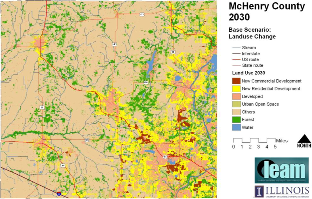
Figure 1.
Summary of land-use change in the business-as-usual scenario. Yellow areas represent new residential development in 2030. Red areas represent new commercial development in 2030.
Future land-use patterns simulated in the enhanced-transportation scenario indicate more growth around the new interchange and less in other parts. While this might be expected to happen in a general sense, the locations for and extents of these gains and losses relative to business-as-usual is not something that can be intuited. Figure 2 is a map that depicts these differences. It compares the two scenarios after aggregating the new acreage in each scenario to quarter sections (1/4 mile square). We find that stakeholders can better comprehend differences among scenarios when the information is aggregated to these larger spatial units. Each quarter section is colored based on the difference between the acreage forecasted in the two scenarios. Quarter-sections colored blue see more acres developed in the enhanced-transportation scenario, while those colored red see more acres developed in the business-as-usual scenario. The intensity of the color depicts the magnitude: darker means greater change. The preponderance of blue quarter-sections in the southwest corner of the county in Fig. 3 indicates more acres developed in this location in the enhanced-transportation scenario; the red quarter sections nearby and around the rest of the county indicate greater acres developed in the business-as-usual scenario. The red quarter sections are essentially places where development would have taken place if the transportation improvements had not been made.
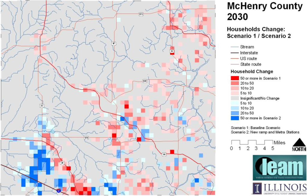
Figure 2.
Difference between two scenarios in terms of acreage added in each quarter section. Blue areas have more acreage in the enhanced-transportation scenario, red areas more acreage in the business-as-usual scenario. Darker colors mean greater differences.
Since land-use change is simulated at a fine spatial resolution (i.e., 30 × 30 meters), it can be aggregated to any desired spatial unit—watershed, school district, governmental jurisdiction, natural-area corridor, and traffic analysis zone—and comparisons can be made between scenarios using that unit of spatial analysis. Figure 3 is a comparison of acres developed in watersheds between the business-as-usual and the enhanced-transportation scenarios. Watersheds close to the new interchange see more development while watersheds elsewhere see less. This suggests that in the future, if the interchange is built, then particular attention will have to be paid to the extent and nature of development in these watersheds.
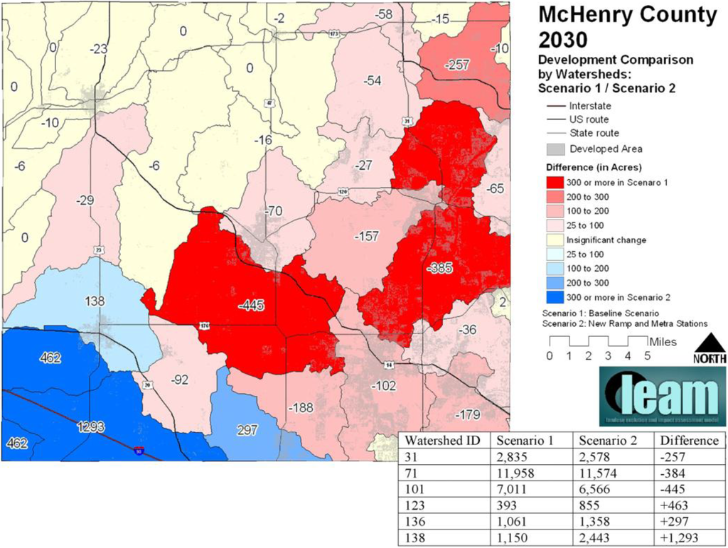
Figure 3.
Difference between two scenarios in terms of new development in watersheds. Blue areas have more acreage in the enhanced-transportation scenario, red areas more acreage in the business-as-usual scenario.
In general, participants in the process found the resulting land-use change scenarios plausible. Where these scenarios were not plausible, either the simulation was incorrect or participants had to give up closely held beliefs. For instance, development along a major arterial (Illinois Route 47, in the middle of the southern part of the county) was much less than was expected. Input data and model assumptions were scrutinized and it turned out that the traffic associated with this particular road was incorrectly represented and the road was less attractive to development. In another example, several small towns in the vicinity of the proposed new interchange expected to see significant development if the interchange were to be built. The amount and location of new development in the enhanced-transportation scenario was not as much as expected and appeared counter-intuitive to them. As discussions of this apparent error in the simulation evolved among participants, the logic of why this was happening was revealed: development was being drawn to the road directly connected to the new interchange rather than the road on which these towns were located. Given this explanation, participants found it easier to believe in the scenario.
With characterizations of ecosystem services and future land-use patterns in hand, we now assess future impacts on these ecosystem services. Rather than use the simple overlay as we did in the Peoria case above, in McHenry we used the more fine-grained approach described earlier for all except one of the ecosystem services studied. To recap: the development likelihood scores for areas associated with an ecosystem service, which are computed internally within the land-use change model, can be used as a measure of the pressure on these areas to change use. This measure can be used to identify areas that are most under pressure or to understand how the pressure to change varies between scenarios.
4.2.1. Prime farmlands
As discussed earlier, areas with LESA scores above 90 were designated prime farmland. The amount of prime farmland that had high development likelihood scores (the top 25%) was slightly higher (1,400 acres or 567 hectares) in the enhanced-transportation scenario but the location and the configuration of these areas is quite different. Figure 4 captures the differences between the two scenarios in terms of the development likelihood of prime farmlands. Red areas will be under greater development pressure in the enhanced-transportation scenario, blue areas under greater pressure in the business-as-usual scenario. Not only are the two areas located very differently (red areas are concentrated in the southwest corner; blue areas are spread out over the rest of the county) but the configuration of these is very different: the red areas are consolidated (and thus more valuable) while the blue areas are extremely fragmented.
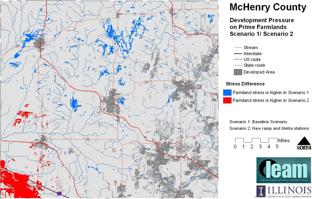
Figure 4.
Difference between two scenarios in terms of development pressure on prime farmlands. Blue areas will experience greater development pressure in the business-as-usual scenario, red areas will experience greater pressure in the enhanced-transportation scenario.
4.2.2. Wetlands
The area of wetlands that had high development likelihood scores (the top 25%) was slightly lower (380 acres or 154 hectares) in the enhanced-transportation scenario. Building the interchange and the railway stations could reduce the amount of wetlands under threat of development but this difference represents just under 1% of the total area of wetlands in the county. The table in Figure 5 shows the distribution of the region’s wetlands in four different categories of development pressure; the map shows how the impact will be differentially located in space with red areas under greater development pressure in the enhanced-transportation scenario, while blue areas under greater pressure in the business-as-usual scenario. The impacts of development are concentrated in the southwest corner of the county in the enhanced-transportation scenario.
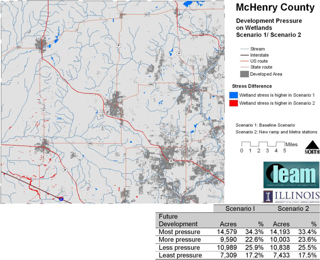
Figure 5.
Difference between two scenarios in terms of development pressure on wetlands. Blue areas will experience greater development pressure in the business-as-usual scenario, red areas will experience greater pressure in the enhanced-transportation scenario.
4.2.3. Threatened and endangered species
As seen in Figure 6, the enhanced-transportation scenario will result in development pressure on 21 of the many quarter-sections where threatened and endangered species have been found. All these areas likely to develop are located in the southwest corner of the county, which is not surprising. None of these areas is under greater development pressure in the business-as-usual scenario.
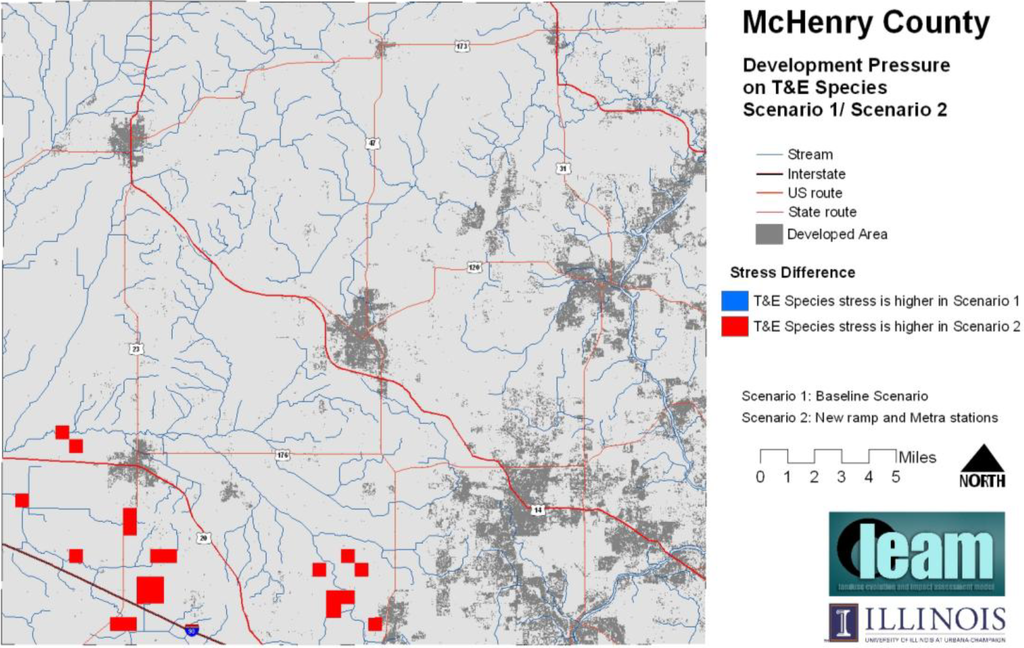
Figure 6.
Difference between two scenarios in terms of development pressure on areas containing threatened and endangered species. Red areas will experience greater development pressure in the enhanced-transportation scenario.
4.2.4. Habitat
In Figure 7, the areas shown in pale green were identified as important core and connective habitat using the approach described earlier. Overlaid on these areas is future development as simulated in the business-as-usual scenario and differentiated over time: current development is in light gray and future development is in black. This suggests that future development is likely to eat away at the margins of these habitat areas in some locations. In two locations in the southeastern part of the county, however, significant portions of connective habitat are likely to be destroyed. These impacts are likely to happen later in the simulation time horizon, i.e., closer to the year 2030. There were not significant differences when the enhanced-transportation scenario was overlaid on the habitat areas; a bit more habitat was destroyed around the new interchange, while slightly less destroyed in other parts of the region.
4.2.5. Summary
Our assessment identifies locations across the county where specific ecosystem services are likely to be affected by future urban development. Some of the consequences of knowing this have emerged in conversations with stakeholders. For instance, the current McHenry County conservation ordinance essentially constrains development on most of the land in the county because there was not a basis for being more selective. The information developed in this assessment allows the ordinance to be applied more stringently and at the same time more focused spatially. Also, with the knowledge provided by this assessment, policymakers choosing among policy and investment options can take into consideration areas that will be affected if these options are implemented.
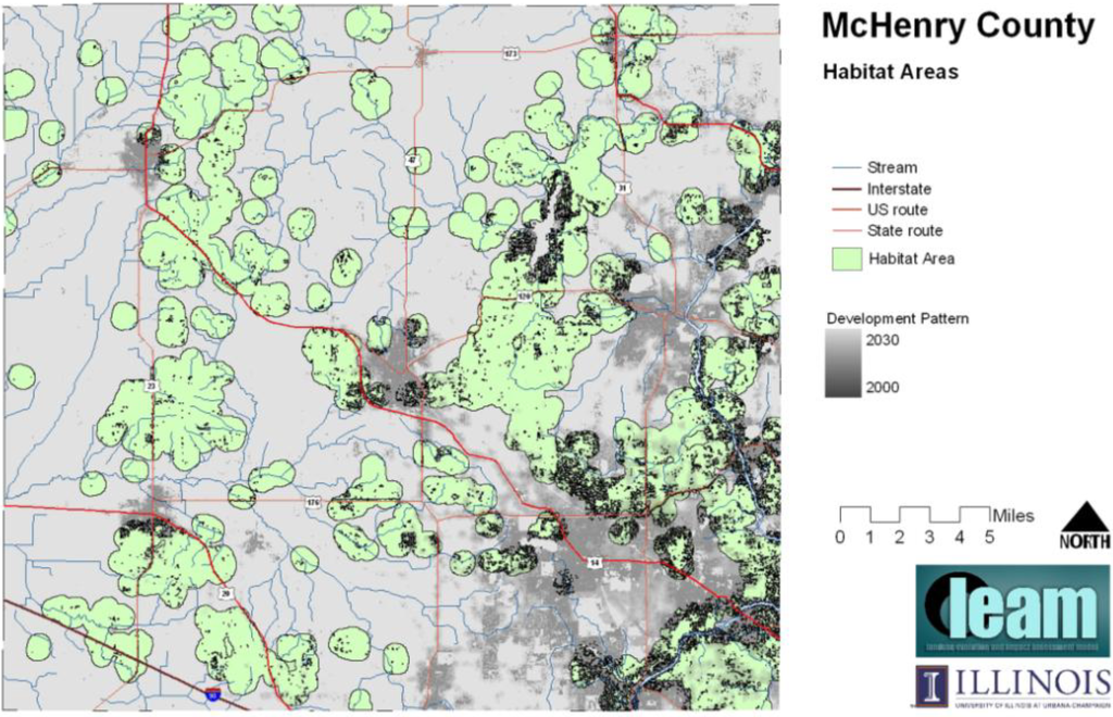
Figure 7.
Sensitive habitat areas and future land-use patterns in the business-as-usual scenario. Green areas are habitat areas. Grey areas depict current and near-term urban development; black areas are development that takes place later in the simulation.
This kind of assessment also allows policy and investment choices to be made with broader sustainability considerations. These choices are usually weighed using very narrow cost-benefit criteria and in the face of appeals to emotions: “We’re the only county in Illinois to not have a highway interchange.” The total acreage of land involved in delivering many ecosystem services is increased only slightly if the highway interchange is built, and doing so will relieve the pressure on critical lands in other parts of the county. On the other hand, as seen above, the areas in the southwest corner of the county that are affected by this public investment are larger and less fragmented than in other parts of the county and are, for that reason, more valuable. Such judgments are possible because stakeholders can see the differential impacts across space; these kinds of ideas had not emerged in any of the regional conversations before this assessment was made available even if some of the conclusions may appear obvious in a general sense. A new interchange is no longer a priority.
5. Conclusions
In this paper we have described an approach—based on understanding the dynamics of urban systems—for assessing the implications of urban policy and investment decisions on the future delivery of ecosystem services. Stakeholders play a central role in critically reviewing the conclusions drawn at each of the three steps in this approach. At the same time, the information generated in this approach provides a concrete and tangible basis for participants to engage with each other. This engagement could facilitate a more complete assessment of negative or positive outcomes that are removed in time and space from those making the assessments; discounting these temporally and spatially distant outcomes leads to unsustainable choices [21]. There are, of course, other ways of assessing environmental impacts of land-use change [22,23].
Our description of the McHenry county application showed how the analysis can be more fine-grained than the simple overlay used in the Peoria application. However, the analysis need not, and probably should not, simply end with assessing how ecosystem services are likely to be affected by a limited set of land-use futures. Rather, additional simulations of future land-use change can be undertaken to elicit the consequences for ecosystem services in general of any actions being contemplated to protect a particular ecosystem service, as was the case in Peoria. For instance, in McHenry county, we simulated land-use change if all the areas that can serve as habitat (shown in green in Figure 7) are protected by being made off-limits to development. We found that doing so will likely push future land development to the southwestern corner of the county (an effect similar to that of constructing the new highway interchange) with its attendant undesirable consequences discussed above. Any attempt to protect habitat areas would, thus, require additional protections put in place to limit these unintended consequences.
As is probably evident by now, the approach described here generates a lot of information that can easily overwhelm participants if not managed and presented well. Participants will want to know the assumptions associated with the land-use pattern in a particular simulation; these should be easily accessed and comprehended. Or, they will want to know if a simulation has been produced on the basis of a certain set of assumptions; they should be able to access a scenario that has already been simulated without starting from scratch. This approach also relies on effective representation of spatial-temporal information. Some ways of effectively representing such information, along with some of the challenges faced, have been discussed in [24]. Effective data management and visualization are key in implementing this approach.
Returning to our story from the Champaign-Urbana metropolitan area, and rewinding to the early 1950s or 1960s when the area was not so heavily developed, a study of the services provided by the Boneyard Creek may have identified the creek’s critical role in draining the central portion of the area. Hydrologists may have identified portions of the creek’s watershed that most contribute stormwater runoff. Planners—taking into account the influence of the University as the area’s largest employer, a magnet for associated residential and commercial development, and its location astride the creek—may have identified many of the areas that eventually developed. By combining this information they could have shown stakeholders how future development would locate in areas that would overwhelm the ecosystem’s ability to drain the area. Perhaps they would have been better able persuade stakeholders of the need to more carefully regulate the type and amount of development in critical areas at that point in time rather than spend large sums all these year later in mitigating the problems created by excessive impervious surfaces and limited on-site retention.
References
- Sierra Club. Solving Sprawl: 1999 Sierra Club Sprawl Report; The Sierra Club Foundation: San Francisco, CA, USA, 1999. [Google Scholar]
- Kunstler, J. The Long Emergency; Atlantic Monthly Press: New York, NY, USA, 2005. [Google Scholar]
- Newman, P.; Kenworthy, J. Sustainability and Cities: Overcoming Automobile Dependence; Island Press: New York, NY, USA, 1999. [Google Scholar]
- Ewing, R.R.; Pendall, D.C. Measuring Sprawl and its Impact Volume 1; Smart Growth America: Washington, DC, USA, 2002. [Google Scholar]
- USDA. 1997 National Resources Inventory Report; USDA: Washington, DC, USA, 1997.
- Aurambout, J.P.; Endress, A.G.; Deal, B. A Spatial Model to Estimate Habitat Fragmentation and its Consequences on Long-Term Persistence of Animal Populations. Environ. Monit. Assess. 2005, 109, 1–3. [Google Scholar] [CrossRef] [PubMed]
- Bonan, G.B. Effects of Land Use on the Climate of the United States. Climatic Change 1997, 37, 449–486. [Google Scholar] [CrossRef]
- Pielke, R. Land Use and Climate Change. Science 2005, 3, 1625. [Google Scholar] [CrossRef]
- Feddema, J.; Oleson, K.; Bonan, G.; Mearns, L.; Buja, L.; Meehl, G.; Washington, W. The Importance of Land-Cover Change in Simulating Future Climates. Science 2005, 3, 1674. [Google Scholar] [CrossRef]
- Watson, R. World Bank Scientist. In Presentation to the Environmental Horizons Conference, Champaign, IL, USA, 2007.
- Duerden, F. Translating Climate Change Impacts at the Community Level. Arctic 2004, 57, 204–212. [Google Scholar] [CrossRef]
- Ruth, M. Smart Growth and Climate Change: Regional Development, Infrastructure and Adaptation; Edward Elgar Inc: Northampton, MA, USA, 2006. [Google Scholar]
- Pease, J.R.; Coughlin, R.E. Land Evaluation and Site Assessment: A guidebook for Rating Agricultural Lands, 2nd ed.; Soil and Water Conservation Society: Ankeny, IA, USA, 1996. [Google Scholar]
- Committee for a Sustainable Emerald Coast. INDEX Paint the Region: A Growth Visioning Tool. Available online: http://www.crit.com/documents/ptr.pdf (accessed on 28 June 2009).
- Klosterman, R. The What If Collaborative Planning Support System. Environ. Plan. B-Plan. Design 1999, 26, 393–408. [Google Scholar] [CrossRef]
- Deal, B. Sustainable Land-Use Planning: The Integration of Process and Technology; Academic Publishing: VDM Verlag, Saarbrücken, Germany, 2008. [Google Scholar]
- Waddell, P. UrbanSim—Modeling Urban Development for Land Use, Transportation, and Environmental Planning. J. Amer. Plann. Asso. 2002, 68, 297–314. [Google Scholar] [CrossRef]
- Deal, B.; Pallathucheril, V. The Land Evolution and impact Assessment Model (LEAM): Will It Play in Peoria? In Proceedings of the 8th International Conference on Computers in Urban Planning and Urban Management, Sendai, Japan, May 27-29, 2003.
- Gerend, T.; Tri-County Regional Planning Commission; Peoria, IL, USA. Personal Communication, 2005.
- USDA-NRCS Hydric Soils Technical Note 1. Proper use of Hydric Soil Terminology.
- Gattig, A.; Hendrickx, L. Judgmental Discounting and Environmental Risk Perception: Dimensional Similarities, Domain Differences, and Implications for Sustainability. J. Soc. Issues 2007, 63, 21–39. [Google Scholar] [CrossRef]
- Deal, B.; Schunk, D. Spatial Dynamic Modeling and Urban Land Use Transformation: A Simulation Approach to Assessing the Costs of Urban Sprawl. Ecol. Econ. 2004, 51, 79–95. [Google Scholar] [CrossRef]
- Wang, Y.; Choi, W.; Deal, B. Long-Term Impacts of Land-Use Change on Non-Point Source Pollutant Loads for the St. Louis Metropolitan Area. Environ. Manage. 2005, 35, 194–205. [Google Scholar] [CrossRef] [PubMed]
- Deal, B.; Pallathucheril, V. Engaging the Future: Forecasts, Scenarios, Plans, and Projects; Hopkins, L.D., Zapata, M.A., Eds.; Lincoln Institute for Land Policy: Cambridge, MA, USA, 2007. [Google Scholar]
© 2009 by the authors; licensee Molecular Diversity Preservation International, Basel, Switzerland. This article is an open-access article distributed under the terms and conditions of the Creative Commons Attribution license ( http://creativecommons.org/licenses/by/3.0/).