Automatic Assessment of Crown Projection Area on Single Trees and Stand-Level, Based on Three-Dimensional Point Clouds Derived from Terrestrial Laser-Scanning


Department of Forest and Soil Science, Institute of Forest Growth, University of Natural Resources and Life Sciences (BOKU), Vienna 1190, Austria
*
Author to whom correspondence should be addressed.
Forests 2018, 9(5), 237; https://doi.org/10.3390/f9050237
Submission received: 13 April 2018
/
Revised: 27 April 2018
/
Accepted: 30 April 2018
/
Published: 1 May 2018
(This article belongs to the Special Issue Advances in Precision Forestry)
Abstract
:Crown projection area (CPA) is a critical parameter in assessing inter-tree competition and estimating biomass volume. A multi-layer seeded region growing-based approach to the fully automated assessment of CPA based on 3D-point-clouds derived from terrestrial laser scanning (TLS) is presented. Independently repeated manual CPA-measurements in a subset of the stand serve as the reference and enable quantification of the inter-observer bias. Allometric models are used to predict CPA for the whole stand and are compared to the TLS-based estimates on the single tree- and stand-level. It is shown that for single trees, the deviation between CPA measurements derived from TLS data and manual measurements is on par with the deviations between manual measurements by different observers. The inter-observer bias propagates into the allometric models, resulting in a high uncertainty of the derived estimates at tree-level. Comparing the allometric models to the TLS measurements at stand-level reveals the high influence of crown morphology, which only can be taken into account by the TLS measurements and not by the allometric models.
1. Introduction
The sustainable and precise management of mixed and uneven aged forest stands in a changing environment requires an in-depth understanding of inter-tree competition and species mingling effects. Competition among neighboring trees mainly depends on (1) the tree species; (2) the inter-tree distances formed by the overall spatial tree pattern in a forest stand; and (3) tree parameters like diameter at breast height (DBH), tree height, or crown projection area (CPA) [1,2,3,4]. The information needed to assess these aspects is much higher compared to data provided by large scale forest inventories, despite the fact that catalogues of key attributes surveyed in forest inventories have broadened and that modern survey networks were developed towards multi-purpose forest inventories [5,6,7].
Thus, long-term forest monitoring plots still play a crucial role in forest research [8,9]. Traditionally, a full census is carried out on long-term observation plots. This procedure is time consuming, cost-intensive, and prone to measuring errors [10]. Recorded tree locations are often erroneous because position, distance, and angular errors propagate in consequence of multiple traverses subsequently aligned over longer distances [11]. Tree crown measurements in old growth stands are labour-intensive and imprecise [12] and may be subject to inter-observer bias [13].
Principally, a rapid and automated measurement of objects in the three-dimensional space and the creation of dense 3D-point clouds at a millimeter-resolution are possible using terrestrial laser scanning (TLS) [14,15,16,17]. Different algorithms for the automatic detection of individual trees in 3D-point clouds have recently been developed and provide detection rates clearly exceeding 90% [10,16,18,19]. Existing studies on automatic DBH measurement from TLS point-clouds have reported root mean squared deviations (RMSD) between measured and fitted DBH values ranging from 0.7 to 7.0 cm [10,18,20,21,22]. Thus, the operational use of these techniques for the automated mapping of forest stands can nowadays be justified [10].
TLS has been successfully used for the semi-automatic assessment of single tree crown parameters [23,24,25,26]. However, a fully automatic assessment of CPA is still a challenging task, especially in vertically structured stands, where individual tree crowns overlap, and in cases of noisy point cloud data (e.g., due to wind induced movements of the tree crowns). Thus, estimates of CPA are often derived in practice using allometric relationships between CPA and easy-to-measure auxiliary variables, e.g., DBH [25]. Fitting such allometric models requires crown data measurements for at least several sample trees. However, these measurements may be subject to inter-observer bias [13], so the resulting models may also be biased.
In this research, a multi-layer seeded region growing-based approach is proposed for the fully automated assessment of CPA based on 3D point-clouds derived from TLS. 3D point-cloud data were collected via multi-scan TLS in a 4.08 ha forest stand located in the Lower Austrian pre-Alps. Independently repeated manual CPA measurements for a sub-sample of trees serve as the reference and enable quantification of the inter-observer bias.
We hypothesize that the proposed automatic method of CPA estimation outperforms standard allometric equations, even when calibrated to local data. In addition, the novel technique avoids uncertainties that usually arise from the inter-observer bias associated with traditional manual measurements. Consequently, we expect that the proposed method can easily be adopted in forest monitoring practice, in conjunction with TLS, without the need for further fieldwork and may therefore become a useful tool for precision forestry applications and the monitoring of long-term research plots.
2. Data and Methods
2.1. Experimental Stand
The survey was conducted in a 4.08 ha stand located in the training forest of the University of Natural Resources and Life Sciences, Vienna (BOKU), near the village of Forchtenstein in the Lower-Austrian pre-Alps (approximately 47.68° N, 16.29° E). A detailed description of the stand is provided by Ritter et al. [10].
The experimental stand is characterized by a high vertical structural diversity with respect to tree heights, including a spatially irregularly distributed understory, and by a high species diversity. Overstory trees are approximately 110 years old and are composed of 38% spruce (Picea abies (L.) H. Karst.), 38% beech (Fagus sylvatica L.), 15% fir (Abies alba Mill.), 5% pine (Pinus sylvestris L.), 4% larch (Larix decidua Mill.), and less than 1% of other broadleaf species. Natural regeneration occurs in irregularly arranged clusters consisting of approximately 90% beech and 10% fir. Stem density is 438 trees ha−1. DBH ranges from 10.0 to 67.3 cm, with a mean of 35.0 cm and median of 36.3 cm. Tree heights range from 5.4 to 40.9 m, with a mean of 27.8 m and median of 29.7 m [10].
2.2. Data Collection
In the summer of 2015, a full census of live trees was performed. A total of 1789 trees with a DBH greater than or equal to 10 cm were measured and recorded in a global coordinate reference system, with an accuracy of ±1.02 m [10]. The DBH values of all trees were measured using a diameter tape, and the basal area (BA) of each tree was calculated as .
In the winter of 2015/16, a full terrestrial laser scan of the test stand was performed using a FARO Focus3D X330 (FARO Technologies Inc., Lake Mary, FL, USA) device [26]. Multi-scan mode with a total of 117 scans obtained from different positions was used, and scanning positions were approximately regularly spaced with a mean distance of circa 20 m between two neighboring positions. Exact scanning positions depended on a visual assessment of the local sighting conditions and were defined in the field. The device’s resolution was set to r = 6.136 mm/10 m and the scan quality parameter was set to 4×, producing moderate noise reduction. Styrofoam balls with a diameter of 15 cm were placed on top of monopods at a height of approximately 1 m, so that three Styrofoam balls were visible from every two neighboring scan positions. Single scan raw data were aligned by means of the Styrofoam balls using the software FARO Scene 6.0 (FARO Technologies Inc., Lake Mary, FL, USA) [27]. The aligned scans were then further processed using the software packages LAStools (rapidlasso GmbH, Gilching, Germany) [28] and R (Version 3.3.2., R Foundation for Statistical Computing, Vienna, Austria) [29]. Finally, a dense 3D-point cloud points) of the whole forest stand was obtained and transformed into a global coordinate reference system (EPSG: 31256) by means of 48 georeferenced and permanently marked reference points. For a more detailed description of the procedures, please refer to Ritter et al. [10].
In addition, eight crown radii per tree (azimuth 0°, 45°, 90°, 135°, 180°, 225°, 270°, and 315°) were measured for a total of 132 trees located in the center of the stand using the “tangential-look-up-method” (tangentiale Hochblickmethode) [13,30] in winter 2016/17. Crown radii measurements were independently repeated by three persons to assess possible inter-observer bias.
2.3. Calculation of CPA from Crown Radii Measurements
The eight crown radii () per tree and their corresponding azimuths () represent points on the border of the trees’ CPA in polar coordinates. These were transformed to Cartesian coordinates according to Equation (1).
and are the Cartesian x- and y-coordinates of a point on the trees’ CPA border, respectively, and and are the Cartesian x- and y-coordinates of the tree, respectively.
2.4. Allometric Models
Allometric models (Equation (2)) with two coefficients () were first developed by Snell [33] and Huxley [34]. Nowadays, allometric models are a common method for the estimation of CPA based on easily measurable proxy variables like basal area (BA) [30].
The underlying differential equation (Equation (3)) reveals that the scaling coefficient describes the relative growth ratio of CPA and BA. indicates isometric scaling, whereas and indicate negative and positive allometric scaling, respectively.
The allometric model (Equation (2)) was linearized to:
and fitted to each of the three independent CPA measurement samples of 132 trees (38 deciduous and 94 coniferous) using ordinary least squares, separated for the two species groups. The fitted models were used to obtain three independent predictions of the CPA for all 1789 trees in the stand.
2.5. Multi-Layer Seeded Region Growing for CPA Assesment
Prior to the application of the multi-layer seeded region growing algorithm, the complete point cloud was height-normalized and split into 65 tiles of a 50 m × 50 m edge length and with an additional 20 m buffer on each side using the LAStools software. These tiles were exported in xyz format so that further data analysis could be processed in R.
The point cloud of each tile was stratified into horizontal layers, each having a vertical extent of 2.5 m. The bottom of the lowest layer was placed at 3.75 m above normalized zero height, so that the central height of that layer was at 5 m. Additional layers were stacked without overlap or gap, until the maximum of the tiles’ z-coordinate was included. Depending on the tile, this procedure resulted in a set of layers with being the layer number in ascending order.
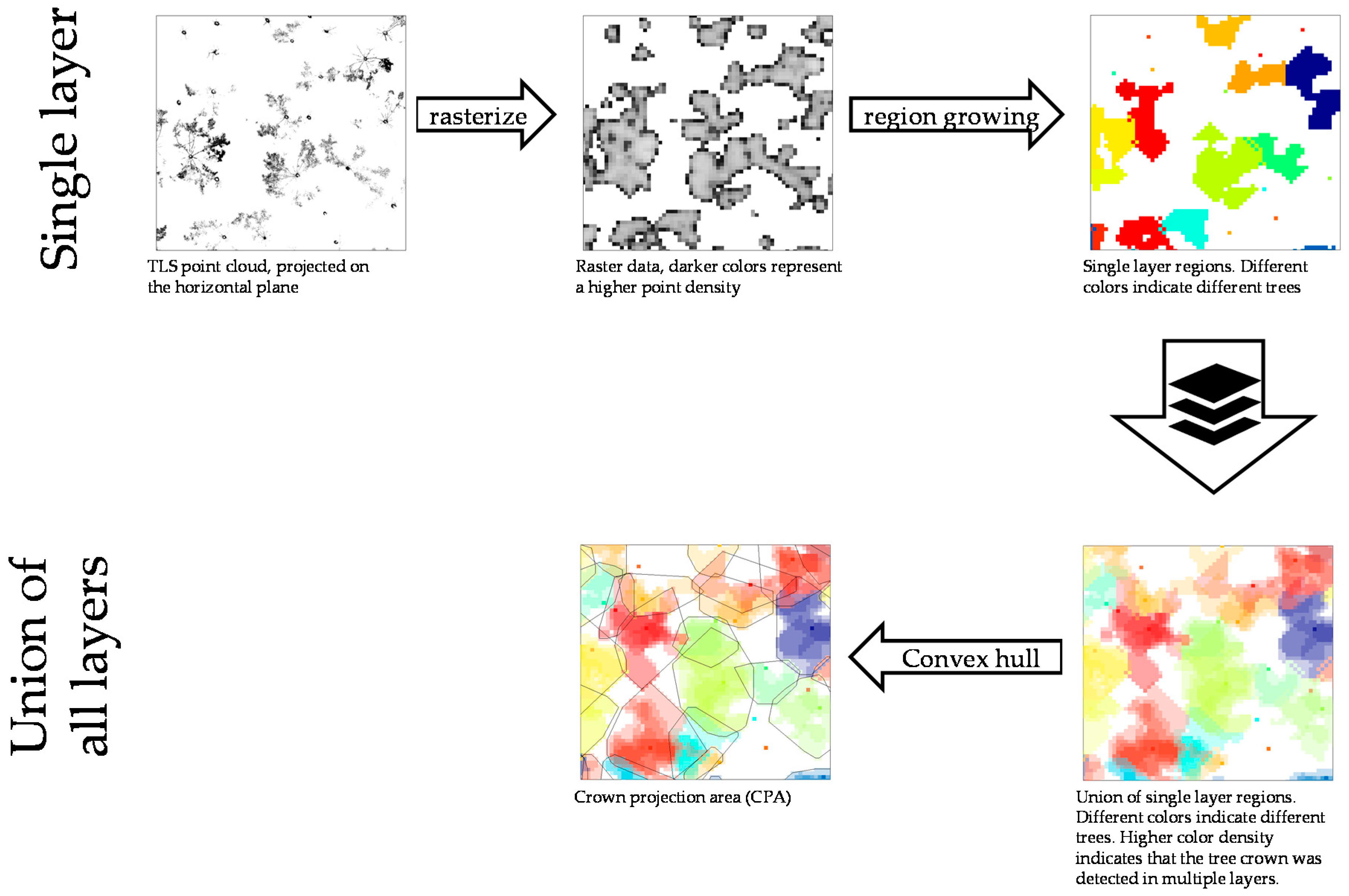
The points within the -th layer where then projected on the horizontal plane. The resulting 2-D point pattern was rasterized with a 25 cm 25 cm pixel size and pixel values according to the number of points within each pixel using the “pixelate” function of the R-package spatstat [32].
A seeded region growing [35] algorithm was applied with seeds corresponding to the tree positions estimated from the 3D point cloud using the two-stage density-based clustering technique described in [10]. The matching of tree coordinates obtained by the full census and from the TLS data was done by a sub-pattern assignment algorithm [10] implemented in the R-package spatstat [32]. For the whole stand, the automatic detection rate was 94.3%, and the corresponding overall accuracy was 91.6% [10]. The 132 target trees, for which CPA was measured manually, were located in the center of the stand. Due to the absence of disturbing edge effects, the automatic detection rate and overall accuracy increased to 98.5% for these trees. Missed and falsely detected trees were manually corrected using the full census data.
In the upper layers, trees were excluded from being used as a seed if their DBH [cm] was smaller than 0.5 times the layer’s central height [m], (i.e., if ), implying the assumption of a maximum possible height-diameter ratio .
If a seed falls within a pixel having a value , this pixel forms an initial seed region with j being the seed number. All unallocated pixels with a value greater than 0 () that share at least a single edge with a seed pixel jointly form the set:
where represents the set of the four direct neighbors.
In every step of the seeded region growing algorithm, all are assigned to their neighboring region (). In case an unallocated pixel has more than one neighboring region, it is assigned to a specific according to the grid order (i.e., starting from the top left and then going row-wise down to the bottom right). The new state of the regions serves as the input for the next iteration, and the procedure is continued as long as there are unallocated pixels with a value greater than 0 that border a region (i.e., as long as ). In order to avoid unrealistic large CPA estimates due to edge effects near the stand border, the procedure was terminated after a maximum of 35 iterations.
The procedure outlined above was repeated for all layers. The total region of tree was then given by , i.e., the spatial union of all corresponding .
The CPA of tree was estimated analogously to the manual measurements, i.e., by the size of a convex hull around . Finally, data from all 65 tiles were re-merged, yielding a representation of the entire experimental stand.
A flowchart of the entire procedure is presented in Figure 1.
3. Results
3.1. CPA Measurements and Inter-Observer Bias for Single Trees
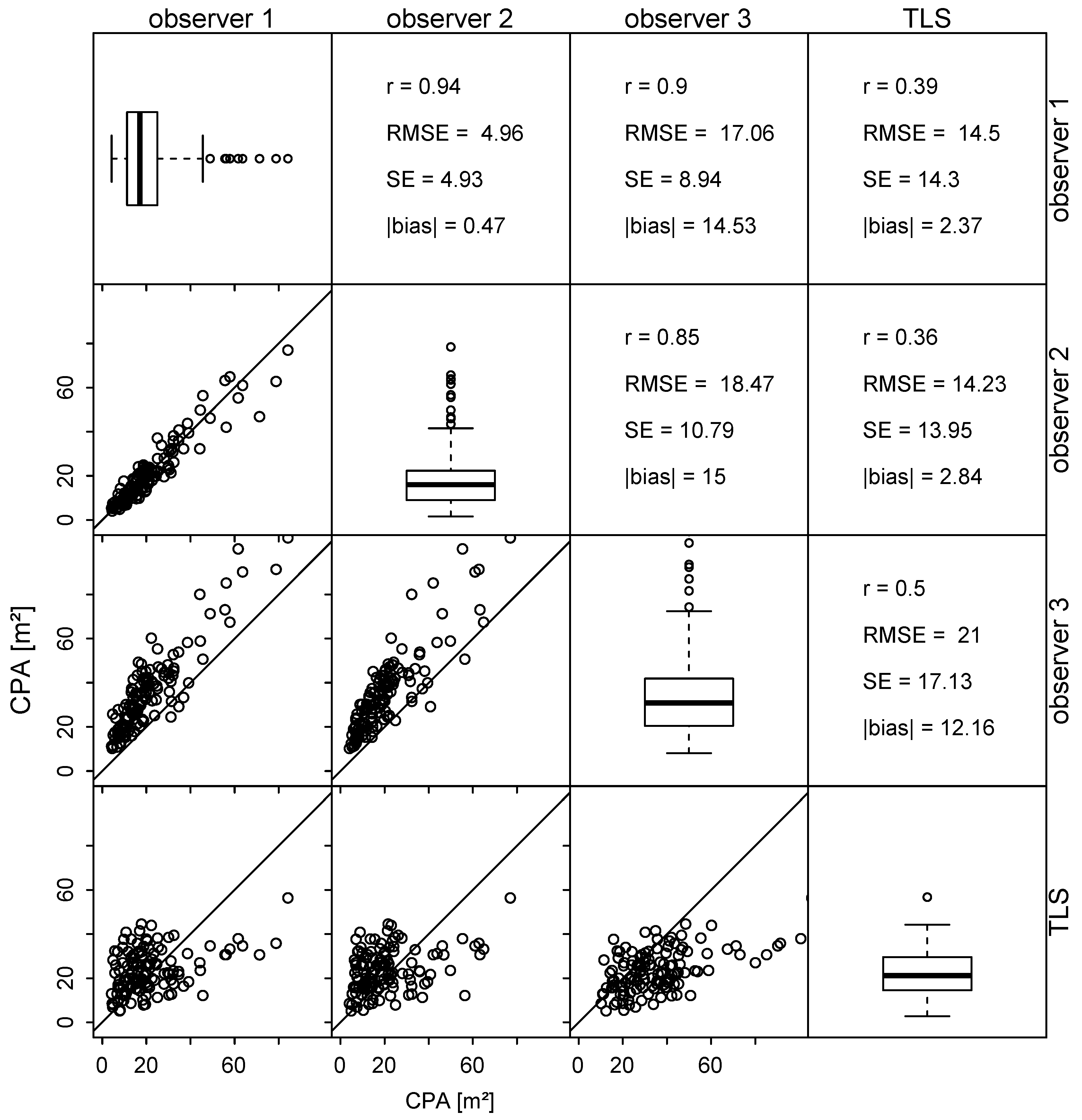
CPA measurements of observer 1 and observer 2 were very similar (RMSE = 4.96 m2) and almost unbiased (estimated |bias| = 0.47 m2). However, there were remarkable inter-observer biases between observer 3 and observers 1 and 2 together (estimated |bias| = 14.53 m2 and 15.00 m2 respectively). The linear relationship between CPA measurements obtained by observers 1–3 was high, with Pearson’s correlation coefficient exceeding 0.85 for all pairs. In contrast, the correlation between the measurements obtained by the three observers and the TLS measurements was comparably low ( ranges between 0.36 and 0.5). Especially for the larger trees, the TLS measurements were systematically lower than the measurements obtained by the three observers (Figure 2, bottom row).
A repeated measures analysis of variance indicated statistical significance of the bias estimates (p < 0.0001) between the CPA measurements obtained by the three observers and TLS. The following simultaneous post-hoc tests for general linear hypotheses [36] yielded the Tukey contrasts given in Table 1. Based on a significance level of , the null-hypothesis of non-systematic errors could not be rejected for two pairs (observer 1 vs. observer 2 and observer 2 vs. TLS), while it was rejected for all other pairs.
3.2. Allometric Models
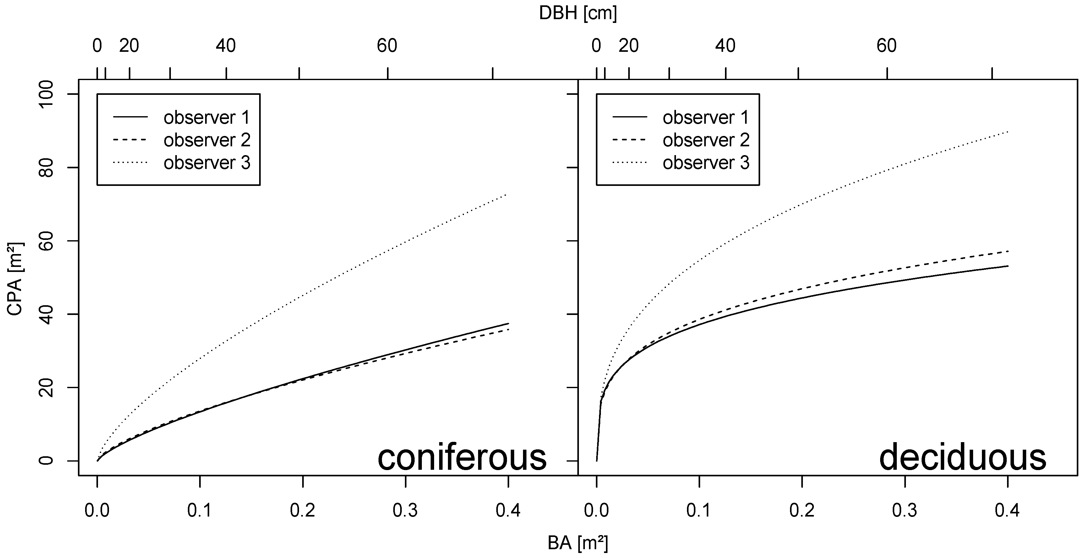
The estimates of of the observer-specific models are more similar for the coniferous trees than for the deciduous trees, while the estimates of the regression coefficient of the observer-specific models are more similar for the deciduous trees than for the coniferous trees (Table 2). Consequently, the shape of the allometric functions (Figure 3) was more similar for the coniferous trees. Here, as an example, the relative difference between the predicted CPA based on the field data of observers 1 and 3, respectively, decreased with increasing DBH (+138% for DBH = 10 cm and +98% for DBH = 60 cm). For the deciduous trees, in contrast, the relative difference between the predicted CPA based on the field data of the two observers increased with increasing DBH (+14% for DBH = 10 cm and +63% for DBH = 60 cm).
The allometric models yielded good results with strong correlations (r > 0.795) and only a little transformation bias (|bias| < 1.69 m2) for the comparison of observed and predicted values from the same observer (Figure 4, main diagonal). However, when comparing the observations of a certain observer with predictions by an allometric model, which was fitted to the observations of a different observer (Figure 4, off-diagonal panels), a maximum absolute bias of 16.38 m2 (observation of observer 1 vs. prediction of observer 3) occurred (corresponding RMSE = 21.1 m2).
The correlations between TLS-derived CPA estimates and the corresponding predictions from the allometric models (Figure 4, right column) were relatively loose (0.226 < r < 0.333). A maximum absolute bias of 10.48 m2 and a maximum RMSE of 17.4 m2 occurred when TLS-based estimates were compared with allometric-model predictions by means of observations from observer 3. Nevertheless, the average difference between TLS-based estimates and observations from observer 3 was still smaller than the difference between predictions obtained by the allometric model fitted to observer 2 data and the actual observer 3 data, and vice versa, respectively.
3.3. CPA Measurements and Inter-Observer Bias at Stand-Level
The different allometric models (Figure 3) fitted to the field data of three independent observers resulted in different estimates of the total CPA (i.e., the sum of all CPAs of single trees) and crown coverage in the forest stand (i.e., the union set of all single tree CPAs). Whereas the crown coverage estimates were very similar for observers 1 and 2, the estimate by means of observer 3 data and the corresponding allometric model was approximately 66% higher. The estimate obtained from the TLS data lied within the range of the allometric model-based estimates (Table 3).
The TLS-based estimates of the total crown coverage were much higher compared to the estimates based on the allometric models and, consequently, the TLS-based estimate of the total gap area was much lower (Table 3).
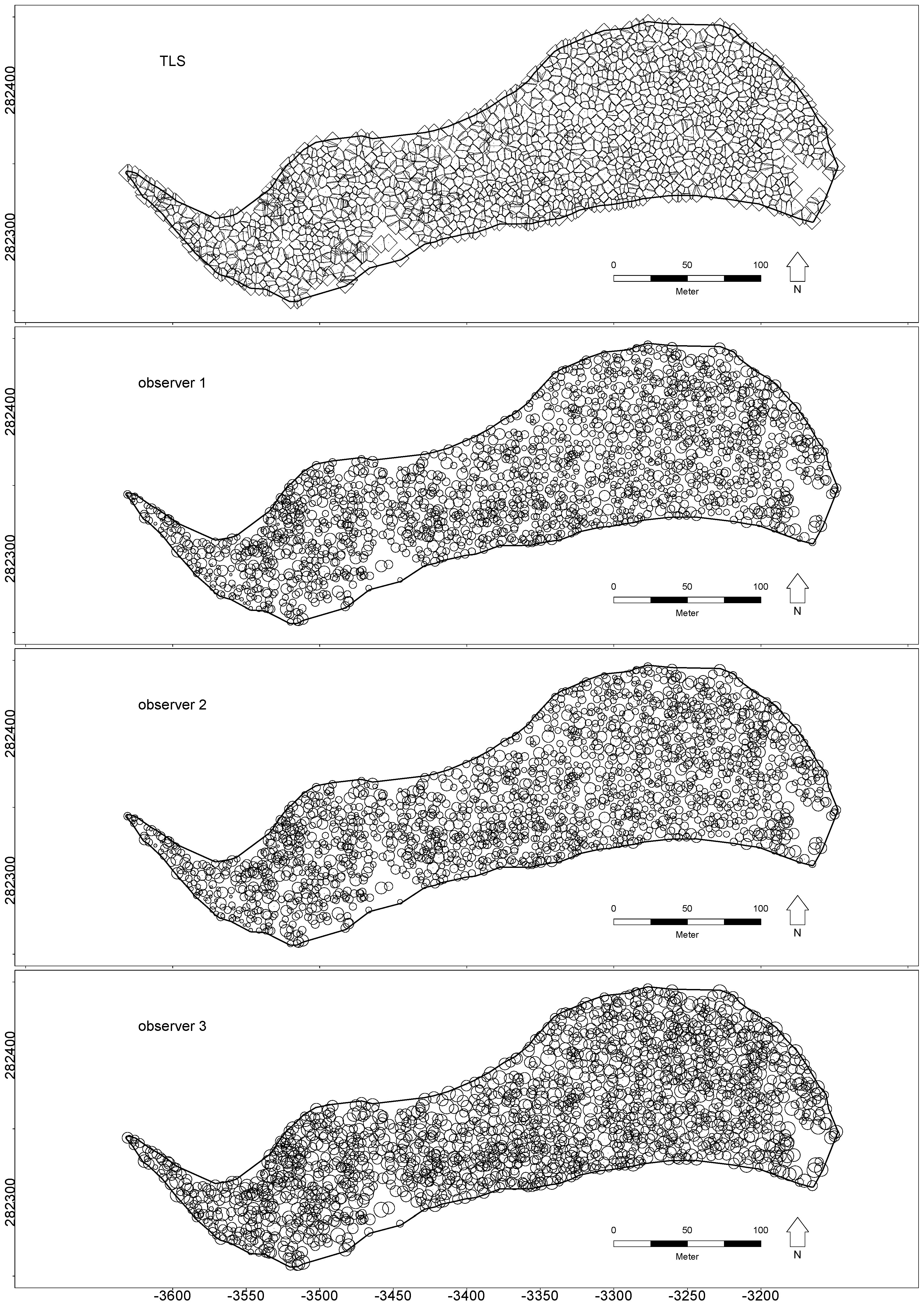
CPA maps derived from the TLS data and the different allometric models are presented in Figure 5, providing a graphic representation of the results from Table 3. While single tree CPA is represented by polygons of different shapes in the map based on the TLS data, it is represented by circles in the maps derived from the allometric models as these models do not yield any information on the shape of the CPA.
4. Discussion
4.1. Multi-Layer Seeded Region Growing versus Other Modelling Approaches
Multi-layer seeded region growing is a rather simplistic approach to CPA modelling compared to other, more complex approaches like quantitative structure models (QSMs) (e.g., [11,22,36,37,38]). However, these complex approaches depend on the availability of high quality data and their implementations are (still) only semi-automatic so that manual intervention is needed. In contrast, the approach presented in this research is fully automated and can deal with more noisy data. Due to non-optimal scanning conditions (i.e., wind) and small errors resulting from the co-registration, the point cloud used for this research is somewhat noisy, especially in the canopy. Moreover, the distance between two neighboring scanning positions is rather long (approximately 20 m), so that shading and self-occlusion become an issue, especially for smaller branches. However, sampling a 4.08 ha stand with a total of 1789 trees requires a fully automated approach and some concessions in regard of the sampling density due to working time limitations.
A possible problem of the classic seeded region growing algorithm [35] is the assignment of pixels to a seed region in case of more than one neighboring region, as that is simply done according to the grid order. Consequently, results may differ depending on the grid order. However, this possible problem was a non-issue for the dataset used in this research, as the grid-order dependent differences were <0.5% for individual tree crowns and stand-level estimates. Thus, an improved version of the algorithm [39], avoiding the grid-order dependency at the costs of computation intensity, was disregarded.
A further possible limitation of the region-growing algorithm occurs when neighboring tree crowns overlap. In that case, single pixels may contain points belonging to two (or more) different trees. Therefore, assigning these pixels to two (or more) regions is desirable. However, it is impossible with standard region growing algorithms. Fuzzy logic-based approaches [40,41] may provide a possible alternative here. However, they were disregarded from this study as trials have shown no better results than for the much simpler approaches. Combining the seeded region growing results from the multiple layers helps to overcome this problem and also yield overlapping CPAs (Figure 5, top row and Table 3).
4.2. Sensor
A terrestrial laser scanner was used to obtain the point cloud. Principally, it should be feasible to use the proposed algorithm together with point cloud data obtained with other sensors, such as mobile laser scanners [42,43] or close range photogrammetry [44,45,46,47,48], as long as a comparable point-cloud density is achieved. For point clouds with a lower density, e.g., obtained from airborne laser scanning (ALS), other approaches are required [49,50,51,52,53].
4.3. Inter-Observer Bias
In this research, a remarkable inter-observer bias was noticed between observer 3 and observers 1 and 2 together, while there was no statistically significant bias between observers 1 and 2. These findings correspond with the results of Röhle [13], who reports inter-observer biases of up to 87.2%. Interestingly, however, between 28% (foliated stand) and 72% (defoliated stand) of the observers yielded approximately unbiased results. Röhle [13] concluded that visual assessment of tree crowns under defoliated conditions is especially difficult and that the inter-observer bias is either almost non-existing or very pronounced, depending on the individuals. Thus, the inter-observer biases illustrated in this study can be regarded as a rather typical phenomenon for manual CPA measurements. Reproducibility of the results from manual CPA measurements, therefore, seems very questionable if different observers are involved. The usage of sensor techniques like TLS will certainly be advantageous from this perspective. However, we did not actually test for a possible intra-observer bias in case the same observer performs the repeated measurements. Hemery et al. [54] reported crown radii measurements “to be repeatable to the nearest 10 cm”; however, they did not report the sample size nor how often measurements were repeated.
4.4. Allometric Model-Fits
The linearized form of the allometric model (Equation (4)) was used for ordinary least squares-based model fitting. While the model fit is unbiased on the log-scale, the retransformation to the normal scale introduces a small transformation bias (Figure 4, main diagonal). Alternative approaches for model fitting (e.g., non-linear least squares techniques) were disregarded due to the small size of the transformation bias.
The allometric models yielded reasonably good results with a strong correlation and small absolute bias when comparing the observed and predicted values from a single observer (Figure 4, main diagonal). This is not surprising as the models were fitted to these data. However, when comparing the predicted values of one observer to the observations of one other (Figure 4, beside the main diagonal), it becomes apparent that the allometric models can only be as good as the field data used for model fitting, as a possible observer related bias from the field data measurements propagates into the allometric models. Thus, caution and independent control measurements must be advised if field data is collected to fit allometric models.
4.5. Crown Morphology
TLS-based estimates of fractional crown cover (Table 3) and related metrics (i.e., crown cover area and gap area) show a remarkable difference compared to the estimates based on the allometric models. However, one has to be reminded that the allometric models used in this study do not reflect the crown morphology. Instead, a tree’s CPA is represented by a circle, i.e., the most compact geometric form in two-dimensional space. Recent studies [55,56] have shown that, especially in mixed-species stands, crown plasticity enables trees to optimize canopy packing, to reduce inter-tree competition, and to maximize the utilization of available photoactive radiation. Obviously, the CPA map (Figure 5) derived from the TLS data represents a much more efficient usage of the growing space than the maps derived from the allometric models. Furthermore, the unanimous perception of all field crews was a closed canopy cover with only two considerably large gaps (one near the eastern stand border and one in the western part of the stand, near the southern border). This corresponds very well with the TLS-based CPA map (Figure 5, top row) and contradicts the CPA maps derived from the allometric equations (Figure 5, rows 2–4).
CPAs derived from the TLS data show a surprisingly regular form for trees located near the stand border. This happened if the region growing algorithm was terminated because the maximum number of iterations was reached. Limiting the maximum number of iterations was necessary due to edge effects. In the neighboring stands, no initial seed regions were defined. Consequently, without limitation of the iterations, the canopy of trees outside the stand would be assigned to trees near the stand borders. Measuring tree positions to define initial seed regions in a buffer zone around the experimental stand would be necessary to avoid these kind of edge effects.
5. Conclusions
It has been shown that multi-layer seeded region growing based on TLS-derived point clouds can be used to asses CPA on single trees and on stand-level. For single trees, the deviation between CPA measurements derived by TLS and manual measurements is on par with the deviations between manual measurements by different observers. Considerations regarding working time and reproducibility suggest an advantage of TLS over the manual measurements.
Allometric models can only be as good as the field data used for model fitting, as a possible inter-observer bias from the field data propagates into the models. Thus, caution and independent control measurements must be advised if field data is collected for model fitting. Due to the fact that the allometric models do not reflect the crown plasticity, estimates of fractional crown cover and related metrics on the stand-level differ remarkably between TLS and allometric models. In mixed-species stands (like the experimental stand) where crown plasticity is pronounced [55,56], TLS is, therefore, clearly the preferable method.
Author Contributions
A.N. planned the experiment together with T.R. and supported manuscript writing. T.R. planned the experiment together with A.N., supervised the field work, performed data analysis and interpretation, and wrote the manuscript.
Acknowledgments
The authors are grateful to Josef Gasch, head of the BOKU Forest Demonstration Centre, for his kind support and cooperativeness during the installation of the test site. The authors appreciate the careful field work of Josef Paulic, Rudolph Feichter, Magdalena Höhne, Clemens Wassermann, Christoph Gollob, Raphael Kostjak, and Florian Brunner.
Conflicts of Interest
The authors declare no conflict of interest.
References
- Bella, I.E. A new competition model for individual trees. For. Sci. 1971, 17, 364–372. [Google Scholar]
- Opie, J.E. Predictability of individual tree growth using various definitions of competing basal area. For. Sci. 1968, 14, 314–323. [Google Scholar]
- Vieilledent, G.; Courbaud, B.; Kunstler, G.; Dhôte, J.F.; Clark, J.S. Individual variability in tree allometry determines light resource allocation in forest ecosystems: A hierarchical Bayesian approach. Oecologia 2010, 163, 759–773. [Google Scholar] [CrossRef] [PubMed] [Green Version]
- Kaitaniemi, P.; Lintunen, A. Neighbor identity and competition influence tree growth in Scots pine, Siberian larch, and silver birch. Ann. For. Sci. 2010, 67, 604. [Google Scholar] [CrossRef]
- Ministerial Conference on the Protection of Forests in Europe (MCPFE). State of Europe’s Forests 2003: The MCPFE Report on Sustainable Forest Management in Europe; Ministerial Conference on the Protection of Forests in Europe (MCPFE) Liaison Unit: Vienna, Austria, 2003. [Google Scholar]
- MCPFE. Background Information for Improved Pan-European Indicators for Sustainable Forest Management; Ministerial Conference on the Protection of Forests in Europe (MCPFE) Liaison Unit: Vienna, Austria, 2003. [Google Scholar]
- IUFRO. Guidelines for Designing Multipurpose Resource Inventories: A Project of IUFRO Research Group 4.02.02; Lund, H.G., Ed.; IUFRO World Series; IUFRO: Vienna, Austria, 1998; Volume 8. [Google Scholar]
- De Vries, W.; Vel, E.; Reinds, G.J.; Deelstra, H.; Klap, J.M.; Leeters, E.E.J.M.; Hendriks, C.M.A.; Kerkvoorden, M.; Landmann, G.; Herkendell, J.; et al. Intensive monitoring of forest ecosystems in Europe: 1. Objectives, set-up and evaluation strategy. For. Ecol. Manag. 2003, 174, 77–95. [Google Scholar] [CrossRef]
- Mellert, K.H.; Deffner, V.; Küchenhoff, H.; Kölling, C. Modeling sensitivity to climate change and estimating the uncertainty of its impact: A probabilistic concept for risk assessment in forestry. Ecol. Model. 2015, 316, 211–216. [Google Scholar] [CrossRef]
- Ritter, T.; Schwarz, M.; Tockner, A.; Leisch, F.; Nothdurft, A. Automatic mapping of forest stands based on three-dimensional point clouds derived from terrestrial laser-scanning. Forests 2017, 8, 265. [Google Scholar] [CrossRef]
- Field, H.L. Landscape Surveying; Delmar, Cengage Learning: Clifton Park, NY, USA, 2012; ISBN 1111310602. [Google Scholar]
- Bayer, D.; Seifert, S.; Pretzsch, H. Structural crown properties of Norway spruce (Picea abies [L.] Karst.) and European beech (Fagus sylvatica [L.]) in mixed versus pure stands revealed by terrestrial laser scanning. Trees Struct. Funct. 2013, 27, 1035–1047. [Google Scholar] [CrossRef]
- Röhle, H. Vergleichende Untersuchungen zur Ermittlung der Genauigkeit bei der Ablotung von Kronenradien. Forstarchiv 1986, 57, 67–71. [Google Scholar]
- Van Leeuwen, M.; Nieuwenhuis, M. Retrieval of forest structural parameters using LiDAR remote sensing. Eur. J. For. Res. 2010, 129, 749–770. [Google Scholar] [CrossRef]
- Liang, X.; Kankare, V.; Hyyppä, J.; Wang, Y.; Kukko, A.; Haggrén, H.; Yu, X.; Kaartinen, H.; Jaakkola, A.; Guan, F.; et al. Terrestrial laser scanning in forest inventories. ISPRS J. Photogramm. Remote Sens. 2016, 115, 63–77. [Google Scholar] [CrossRef]
- Yang, B.; Dai, W.; Dong, Z.; Liu, Y. Automatic forest mapping at individual tree levels from terrestrial laser scanning point clouds with a hierarchical minimum cut method. Remote Sens. 2016, 8, 372. [Google Scholar] [CrossRef]
- Srinivasan, S.; Popescu, S.C.; Eriksson, M.; Sheridan, R.D.; Ku, N.-W.; Waser, L.T.; Wynne, R.H.; Thenkabail, P.S. Terrestrial laser scanning as an effective tool to retrieve tree level height, crown width, and stem diameter. Remote Sens. 2015, 7, 1877–1896. [Google Scholar] [CrossRef]
- Maas, H.-G.; Bienert, A.; Scheller, S.; Keane, E. Automatic forest inventory parameter determination from terrestrial laser scanner data. Int. J. Remote Sens. 2008, 29, 1579–1593. [Google Scholar] [CrossRef]
- Xia, S.; Wang, C.; Pan, F.; Xi, X.; Zeng, H.; Liu, H. Detecting stems in dense and homogeneous forest using single-scan TLS. Forests 2015, 6, 3923–3945. [Google Scholar] [CrossRef]
- Brolly, G.; Kiraly, G. Algorithms for stem mapping by means of terrestrial laser scanning. Acta Silv. Lign. Hung. 2009, 5, 119–130. [Google Scholar]
- Liang, X.; Hyyppä, J. Automatic stem mapping by merging several terrestrial laser scans at the feature and decision levels. Sensors 2013, 13, 1614–1634. [Google Scholar] [CrossRef] [PubMed]
- Olofsson, K.; Holmgren, J.; Olsson, H. Tree stem and height measurements using terrestrial laser scanning and the RANSAC algorithm. Remote Sens. 2014, 6, 4323–4344. [Google Scholar] [CrossRef]
- Calders, K.; Newnham, G.; Burt, A.; Murphy, S.; Raumonen, P.; Herold, M.; Culvenor, D.; Avitabile, V.; Disney, M.; Armston, J.; et al. Nondestructive estimates of above-ground biomass using terrestrial laser scanning. Methods Ecol. Evol. 2015, 6, 198–208. [Google Scholar] [CrossRef]
- Dassot, M.; Constant, T.; Fournier, M. The use of terrestrial LiDAR technology in forest science: Application fields, benefits and challenges. Ann. For. Sci. 2011, 68, 959–974. [Google Scholar] [CrossRef]
- Barbeito, I.; Dassot, M.; Bayer, D.; Collet, C.; Drössler, L.; Löf, M.; del Rio, M.; Ruiz-Peinado, R.; Forrester, D.I.; Bravo-Oviedo, A.; et al. Terrestrial laser scanning reveals differences in crown structure of Fagus sylvatica in mixed vs. pure European forests. For. Ecol. Manag. 2017, 405, 381–390. [Google Scholar] [CrossRef]
- FARO Laser Scanner FARO Focus3D—Overview—3D Surveying. Available online: http://www.faro.com/en-us/products/3d-surveying/faro-focus3d/overview (accessed on 28 February 2017).
- FARO FARO Laser Scanner Software—SCENE—Overview. Available online: http://www.faro.com/en-us/products/faro-software/scene/overview (accessed on 28 February 2017).
- Isenburg, M. LAStools—Efficient LiDAR Processing Software (Version 160429, Academic). Available online: https://rapidlasso.com/lastools/ (accessed on 28 February 2017).
- R Development Core Team. R: A Language and Environment for Statistical Computing. R Version 3.3.2; R Foundation for Statistical Computing: Vienna, Austria, 2016. [Google Scholar]
- Grote, R. Estimation of crown radii and crown projection area from stem size and tree position. Ann. For. Sci. 2003, 60, 393–402. [Google Scholar] [CrossRef]
- Pateiro-Lopez, B.; Rodriguez-Casal, A. Alphahull: Generalization of the Convex Hull of a Sample of Points in the Plane. R package Version 2.1; 2016; Available online: https://cran.r-project.org/package=alphahull (accessed on 12 February 2018).
- Baddeley, A.; Rubak, E.; Turner, R. Spatial Point Patterns: Methodology and Applications with R; Chapman and Hall/CRC Press: London, UK, 2015. [Google Scholar]
- Snell, O. Die Abhängigkeit der Hirngewichte von dem Körpergewicht und den geistigen Fähigkeiten. Arch. Psychiatr. Nervenkr. 1891, 23, 436–446. [Google Scholar] [CrossRef]
- Huxley, J. Problems of Relative Growth; Lincoln Mac Veagh: New York, NY, USA, 1932. [Google Scholar]
- Adams, R.; Bischof, L. Seeded region growing. IEEE Trans. Pattern Anal. Mach. Intell. 1994, 16, 641–647. [Google Scholar] [CrossRef]
- Hothorn, T.; Bretz, F.; Westfall, P. Simultaneous Inference in General Parametric Models. Biometr. J. 2008, 50, 346–363. [Google Scholar] [CrossRef] [PubMed]
- Hackenberg, J.; Spiecker, H.; Calders, K.; Disney, M.; Raumonen, P. SimpleTree—An efficient open source tool to build tree models from TLS clouds. Forests 2015, 6, 4245–4294. [Google Scholar] [CrossRef]
- Hackenberg, J.; Morhart, C.; Sheppard, J.; Spiecker, H.; Disney, M. Highly accurate tree models derived from terrestrial laser scan data: A method description. Forests 2014, 5, 1069–1105. [Google Scholar] [CrossRef]
- Mehnert, A.; Jackway, P. An improved seeded region growing algorithm. Pattern Recognit. Lett. 1997, 18, 1065–1071. [Google Scholar] [CrossRef]
- Wang, C.-M.; Lin, G.-C. A Study on the Application of Fuzzy Information Seeded Region Growing in Brain MRI Tissue Segmentation; Hindawi: New York, NY, USA, 2014; Volume 2014. [Google Scholar]
- Kang, C.-C.; Wang, W.-J. Fuzzy based seeded region growing for image segmentation. In NAFIPS 2009—2009 Annual Meeting of the North American Fuzzy Information Processing Society; IEEE: Piscataway, NJ, USA, 2009; pp. 1–5. [Google Scholar]
- Rutzinger, M.; Pratihast, A.K.; Oude Elberink, S.; Vosselman, G. Detection and modelling of 3D trees from mobile laser scanning data. Int. Arch. Photogramm. Remote Sens. Spat. Inf. Sci. 2010, XXXVIII, 520–525. [Google Scholar]
- Holopainen, M.; Kankare, V.; Vastaranta, M.; Liang, X.; Lin, Y.; Vaaja, M.; Yu, X.; Hyyppä, J.; Hyyppä, H.; Kaartinen, H.; et al. Tree mapping using airborne, terrestrial and mobile laser scanning—A case study in a heterogeneous urban forest. Urban For. Urban Green. 2013, 12. [Google Scholar] [CrossRef]
- Mokroš, M.; Liang, X.; Surový, P.; Valent, P.; Čerňava, J.; Chudý, F.; Tunák, D.; Saloň, Š.; Merganič, J. Evaluation of close-range photogrammetry image collection methods for estimating tree diameters. ISPRS Int. J. Geo-Inform. 2018, 7, 93. [Google Scholar] [CrossRef]
- Bright, B.C.; Loudermilk, E.L.; Pokswinski, S.M.; Hudak, A.T.; O’Brien, J.J. Introducing close-range photogrammetry for characterizing forest understory plant diversity and surface fuel structure at fine scales. Can. J. Remote Sens. 2016, 42, 460–472. [Google Scholar] [CrossRef]
- Mikita, T.; Janata, P.; Surový, P. Forest stand inventory based on combined aerial and terrestrial close-range photogrammetry. Forests 2016, 7, 165. [Google Scholar] [CrossRef]
- Forsman, M.; Börlin, N.; Holmgren, J. Estimation of tree stem attributes using terrestrial photogrammetry with a camera rig. Forests 2016, 7, 61. [Google Scholar] [CrossRef]
- Panagiotidis, D.; Abdollahnejad, A.; Surový, P.; Chiteculo, V. Determining tree height and crown diameter from high-resolution UAV imagery. Int. J. Remote Sens. 2016, 1–19. [Google Scholar] [CrossRef]
- Kaartinen, H.; Hyyppä, J.; Yu, X.; Vastaranta, M.; Hyyppä, H.; Kukko, A.; Holopainen, M.; Heipke, C.; Hirschmugl, M.; Morsdorf, F.; Næsset, E.; et al. An international comparison of individual tree detection and extraction using airborne laser scanning. Remote Sens. 2012, 4, 950–974. [Google Scholar] [CrossRef] [Green Version]
- Hyyppä, J.; Holopainen, M.; Olsson, H. Laser scanning in forests. Remote Sens. 2012, 4, 2919–2922. [Google Scholar] [CrossRef]
- Hyyppä, J.; Yu, X.; Hyyppä, H.; Vastaranta, M.; Holopainen, M.; Kukko, A.; Kaartinen, H.; Jaakkola, A.; Vaaja, M.; Koskinen, J.; et al. Advances in forest inventory using airborne laser scanning. Remote Sens. 2012, 4, 1190–1207. [Google Scholar] [CrossRef]
- Wallace, L.; Lucieer, A.; Malenovsky, Z.; Turner, D.; Vopenka, P. Assessment of forest structure using two UAV techniques: A comparison of airborne laser scanning and structure from motion (SfM) point clouds. Forests 2016, 7, 62. [Google Scholar] [CrossRef]
- Lindberg, E.; Hollaus, M. Comparison of methods for estimation of stem volume, stem number and basal area from airborne laser scanning data in a hemi-boreal forest. Remote Sens. 2012, 4, 1004–1023. [Google Scholar] [CrossRef]
- Hemery, G.E.; Savill, P.S.; Pryor, S.N. Applications of the crown diameter–stem diameter relationship for different species of broadleaved trees. For. Ecol. Manag. 2005, 215, 285–294. [Google Scholar] [CrossRef]
- Jucker, T.; Bouriaud, O.; Coomes, D.A. Crown plasticity enables trees to optimize canopy packing in mixed-species forests. Funct. Ecol. 2015, 29, 1078–1086. [Google Scholar] [CrossRef] [Green Version]
- Longuetaud, F.; Piboule, A.; Wernsdörfer, H.; Collet, C. Crown plasticity reduces inter-tree competition in a mixed broadleaved forest. Eur. J. For. Res. 2013, 132, 621–634. [Google Scholar] [CrossRef]
Figure 1.
Flowchart of the multi-layer seeded region growing procedure. The top-row shows the procedure for a single layer, and the bottom row shows the procedure for the union of all layers. The depicted tile size is 20 m × 20 m.
Figure 1.
Flowchart of the multi-layer seeded region growing procedure. The top-row shows the procedure for a single layer, and the bottom row shows the procedure for the union of all layers. The depicted tile size is 20 m × 20 m.

Figure 2.
Scatter plot matrix of independently repeated crown projection area (CPA) measurements. Root mean squared error (RMSE), standard error (SE), and absolute bias (|bias|) are estimates given in m2. r = Pearson’s correlation coefficient.
Figure 2.
Scatter plot matrix of independently repeated crown projection area (CPA) measurements. Root mean squared error (RMSE), standard error (SE), and absolute bias (|bias|) are estimates given in m2. r = Pearson’s correlation coefficient.

Figure 3.
Comparison of the allometric models for the two species groups (coniferous and deciduous) fitted to the data obtained independently by the three different observers. BA = basal area, DBH = diameter at breast height, and CPA = crown projection area.
Figure 3.
Comparison of the allometric models for the two species groups (coniferous and deciduous) fitted to the data obtained independently by the three different observers. BA = basal area, DBH = diameter at breast height, and CPA = crown projection area.

Figure 4.
Observed CPA vs. CPA predicted by allometric models that were fitted to the field data obtained independently by the three different observers and terrestrial laser scanning (TLS) CPA estimates for n = 132 trees. RMSE, SE, and |bias| are estimates given in m2. r = Pearson’s correlation coefficient.

Figure 5.
Maps of crown projection area derived from terrestrial laser scanning data and allometric models fitted to the field data of three independent observers.
Figure 5.
Maps of crown projection area derived from terrestrial laser scanning data and allometric models fitted to the field data of three independent observers.


Table 1.
Results of the simultaneous post-hoc tests for general linear hypotheses of non-systematic deviations between CPA measurements.
Table 1.
Results of the simultaneous post-hoc tests for general linear hypotheses of non-systematic deviations between CPA measurements.
| Linear Hypotheses | |z-value| | p-Value |
|---|---|---|
| observer 1 − observer 2 = 0 | 0.477 | 0.964 |
| observer 1 − observer 3 = 0 | 14.009 | <0.001 *** |
| observer 1 − TLS = 0 | 2.755 | 0.030 * |
| observer 2 − observer 3 = 0 | 13.532 | <0.001 *** |
| observer 2 − TLS = 0 | 2.279 | 0.103 |
| observer 3 − TLS = 0 | 11.220 | <0.001 *** |
*: ; ***: .
Table 2.
Parameter estimates for the different allometric models.
| Allometric Model (Observer) | Coniferous | Deciduous | ||
|---|---|---|---|---|
| 1 | 73.91 | 0.742 | 67.22 | 0.257 |
| 2 | 67.90 | 0.698 | 74.02 | 0.283 |
| 3 | 137.14 | 0.691 | 124.46 | 0.357 |
Table 3.
Total CPA, total overshadowed area, total gap area, and fractional crown cover estimated from the terrestrial laser scanning (TLS) data and from the allometric models fitted to the field data of three independent observers (n = 1789 trees; stand area = 4.08 ha).
Table 3.
Total CPA, total overshadowed area, total gap area, and fractional crown cover estimated from the terrestrial laser scanning (TLS) data and from the allometric models fitted to the field data of three independent observers (n = 1789 trees; stand area = 4.08 ha).
| Total CPA (m2) | Crown Coverage (m²) | Total Gap Area (m²) | Crown Coverage (%) | |
|---|---|---|---|---|
| observer 1 | 39 088 | 21 124 | 19 653 | 51.8 |
| observer 2 | 39 888 | 21 402 | 19 375 | 52.5 |
| observer 3 | 66 327 | 29 202 | 11 575 | 71.6 |
| TLS | 45 175 | 40 041 | 5 134 | 98.2 |
© 2018 by the authors. Licensee MDPI, Basel, Switzerland. This article is an open access article distributed under the terms and conditions of the Creative Commons Attribution (CC BY) license (http://creativecommons.org/licenses/by/4.0/).
Share and Cite
MDPI and ACS Style
Ritter, T.; Nothdurft, A. Automatic Assessment of Crown Projection Area on Single Trees and Stand-Level, Based on Three-Dimensional Point Clouds Derived from Terrestrial Laser-Scanning. Forests 2018, 9, 237. https://doi.org/10.3390/f9050237
AMA Style
Ritter T, Nothdurft A. Automatic Assessment of Crown Projection Area on Single Trees and Stand-Level, Based on Three-Dimensional Point Clouds Derived from Terrestrial Laser-Scanning. Forests. 2018; 9(5):237. https://doi.org/10.3390/f9050237
Chicago/Turabian StyleRitter, Tim, and Arne Nothdurft. 2018. "Automatic Assessment of Crown Projection Area on Single Trees and Stand-Level, Based on Three-Dimensional Point Clouds Derived from Terrestrial Laser-Scanning" Forests 9, no. 5: 237. https://doi.org/10.3390/f9050237
Note that from the first issue of 2016, this journal uses article numbers instead of page numbers. See further details here.