Regeneration of Native Forest Species in Mainland Portugal: Identifying Main Drivers


Centro de Investigação e Tecnologias Agroambientais e Biológicas, CITAB, Universidade de Trás-os-Montes e Alto Douro, UTAD, Quinta dos Prados, Apartado 1013, 5000-801 Vila Real, Portugal
*
Author to whom correspondence should be addressed.
Forests 2018, 9(11), 694; https://doi.org/10.3390/f9110694
Submission received: 4 October 2018
/
Revised: 3 November 2018
/
Accepted: 6 November 2018
/
Published: 8 November 2018
(This article belongs to the Section Forest Ecology and Management)
Abstract
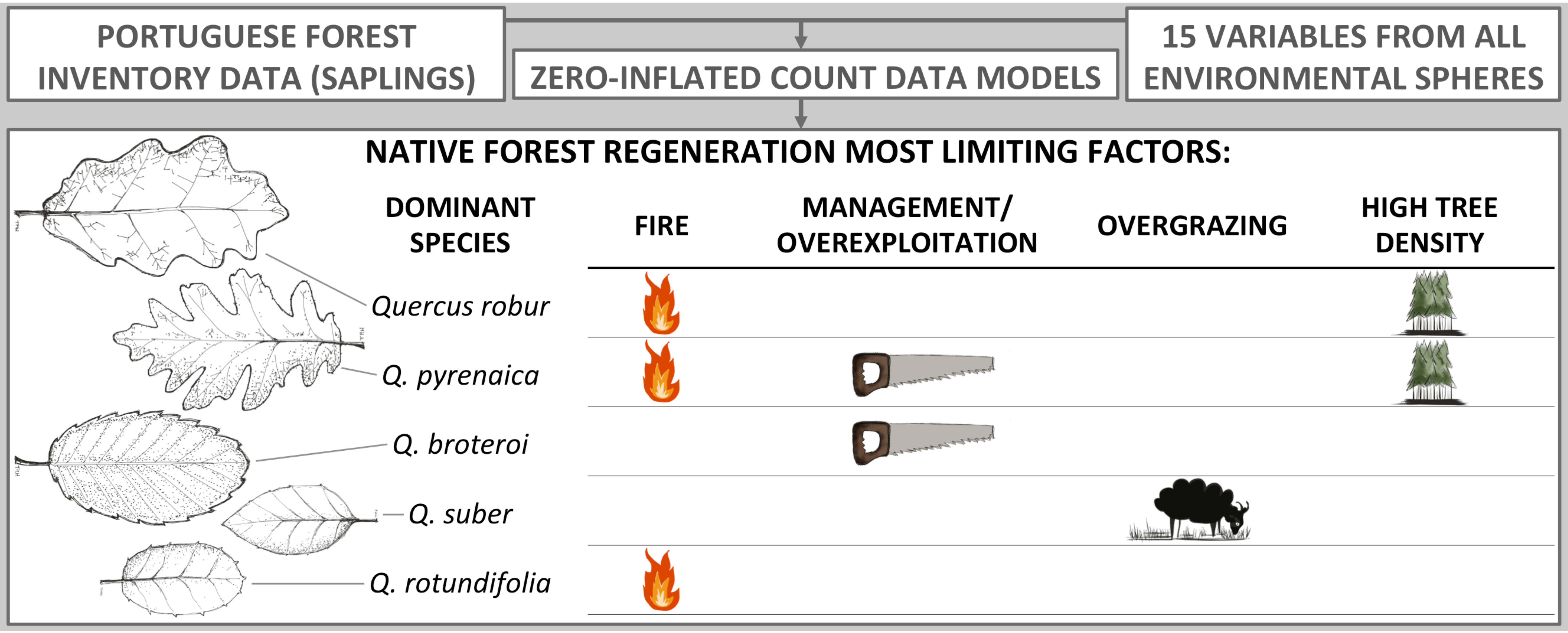
:Persistence of native forests is a global concern. We aimed at unveiling the main factors affecting tree recruitment in Portuguese native forests, modelling sapling data collected during the 5th Portuguese Forest Inventory, for five main Quercus taxa. Zero-inflated count data models allowed us to examine simultaneously (i) the absence of tree recruitment and (ii) the density of tree recruitment. Using Akaike weights, we obtained importance values for 15 relevant explanatory variables. Results showed that seed availability and climatic variables were determinant to understand regional absence of regeneration for all taxa. Seed availability was also an important driver of sapling density, except for Quercus suber. Other variables impacted on regeneration density: grazing hindered Q. suber regeneration; regeneration of Q. rotundifolia and Q. suber was lower in flat areas; recurrent fire hampered the regeneration of Q. robur and Q. pyrenaica; Q. broteroi and Q. pyrenaica showed depressed regeneration in regions where forest plantations abound, while Q. robur and Q. suber seemed selectively protected. We conclude that caution is warranted when analysing pooled data for Quercus spp. regeneration, as different variables affected Quercus taxa differently. Finally, we suggest dedicated management actions to enhance the establishment of new native forests.

1. Introduction
Native forests are of great concern for nature conservation [1]. On the one hand, they are known to shelter significantly more biodiversity than planted forests [2,3,4,5,6,7,8,9]; on the other hand, they have been exploited by man since long and eventually replaced on a large scale with agriculture, urban fabric and other land uses [10].
Native forests are nowadays subjected to new challenges that endanger their long-term persistence, such as regeneration failure [11,12,13], climatic changes [14,15] and replacement with non-native forest species [1]. The latter are already widely distributed in Portugal. Portuguese native forests were reduced to less than 7% of the territory by the end of the 19th century [16,17] and never recovered conspicuously [17,18] for three main reasons: (i) during the first half of the 20th century, Pinus pinaster Aiton was the preferred forestry species [17]; (ii) during the second half of the 20th century, preference was given to the exotic Eucalyptus globulus Labill., which is currently the most abundant forest species in Portugal, corresponding to 26% of the forested areas [17,19]; and (iii) since the end of the 20th century, a great increase in the extent of wildfires [20], which recurrently burn shrublands [21], delaying the progression of ecological succession.
Forest regeneration and its possible failure have long worried scientists [22]. A considerable number of scientific studies have shown that a very large set of variables affects forest regeneration. We list some examples of such variables, non-exhaustively: air temperature [23,24]; moisture [25]; light [26,27,28,29]; aspect [30]; nurse-effect of shrubs or trees [30,31,32]; animal mediated seed dispersal [33,34]; grazing and browsing [23,35]; proximity to seed source [36]; disturbance regimes like those emerging from fire patterns [12,37]; soil nutrients [26,27]; soil organic layer depth [11,38]; soil texture [11]. Modelling forest regeneration is thus challenging, as a vast set of variables is known to possibly affect it. Additionally, the effects of such variables can have opposite signals among different contexts. For example, Caldeira et al. [39] showed that under Mediterranean climate (where summer drought is pronounced), tree canopy cover negatively affected seedlings growth but facilitated seedlings survival of Quercus suber L. and Q. rotundifolia Lam., while low soil moisture, high soil temperature and herb biomass decreased their survival. Similarly, Plieninger et al. [11] have associated Q. suber, Q. rotundifolia and Q. pyrenaica Willd. regeneration failure with more open, uniform, and/or aged woodlands. Conversely, under temperate climate, where water availability is not as limiting, tree regeneration might depend much more on competitive growth and gap-dynamics [29,40,41]. Other variables can have two-fold effects even on the same species under similar contexts, depending on their frequency patterns. for example, relatively infrequent fires can trigger or promote tree regeneration and diversity [42,43,44], while recurrent fires can strongly and negatively affect forest regeneration, eventually compromising it in the long-term [45].
“Foundation species” sensu Dayton [46], constitute fundamental taxa for the structuring of the whole community. Dominant trees are foundation species within the forest ecosystem they thrive in and are intimately connected to the existing biodiversity. Here we approach forest regeneration focusing on dominant tree recruitment. In particular we considered five Quercus taxa that dominate zonal native forests in mainland Portugal, namely: Quercus robur L., Q. pyrenaica Willd., Q. faginea Lam. subsp. broteroi (Cout.) A. Camus, Q. suber L. and Q. rotundifolia Lam. [47]. Although other genera can dominate zonal native forests in mainland Portugal, for example, Juniperus, Pinus, Olea, Ceratonia and Betula [48], the five referred Quercus taxa account for 93% of the potential zonal native forests area in mainland Portugal [47]. Currently, in Portugal, 21.5% of the mainland territory is included in the National System of Classified Areas [49]. However, forests devoted to biodiversity conservation occupy about 145 000 ha [50], representing 4.5% of the forested area and 1.6% of the Portuguese mainland territory, once mostly covered by forests [47,51,52,53,54].
Our single objective is to comprehensively understand the regeneration of these native forest taxa in mainland Portugal, testing a wide collection of high-quality explanatory variables, answering the question: which are the most relevant factors driving tree recruitment in Portuguese native forests? Unveiling such factors is of ultimate importance not only to devise inclusive guidelines targeting the expansion of native forests but also to underpin forest management strategies and best practices.
We concluded that even if some variables affected all the studied taxa similarly, some other variables showed very different relevance between taxa. This allowed us to point out basic dedicated management actions to enhance the establishment of new native forests.
2. Materials and Methods
2.1. Base Data
We used data from the 5th National Forest Inventory (NFI5) [55], which surveyed around 6800 forest plots (of 500 to 2000 m2) on a regular grid (2 × 2 km) within mainland Portugal, during 2005 and 2006. In particular, we used as dependent variable the number of “small trees” of each of the five oak taxa already referred (Q. robur, Q. pyrenaica, Q. faginea subsp. broteroi, Q. suber and Q. rotundifolia). Q. faginea subsp. faginea occurs scattered among Q. suber and Q. rotundifolia forests in the northeast of Portugal [56] and some very rare forests are dominated by this subspecies in the same region [57]. However, since the spatial resolution of NFI5 does not seem sufficient to capture these very rare forests and very little regeneration of that subspecies was recorded, Q. faginea subsp. faginea regeneration was not modelled. Pooling the two subspecies was not an option, given the substantially different conditions (climate, land use, orography) under which they thrive. Henceforth, Q. faginea subsp. broteroi is denoted simply as Q. broteroi. The NFI5 considers as “small trees” those taller than 0.50 m but with a diameter at breast height (1.30 m) inferior to 7.5 cm. Hereafter we denote “small tree” as sapling.
We searched for high-resolution/high-quality variables, as the NFI5 dataset has high spatial accuracy (the maximum admissible positioning error of the plots centre was 6 m). Aiming at covering the widest possible range of variable types, we gathered 15 putative explanatory variables known to affect forest regeneration. We describe these variables in the following paragraphs.
From data collected during the NFI5, we used basal area (G), tree density (N), evidence of grazing (GRAZI) and evidence of understory clearing (UnderClear). Also using data from the NFI5 on the dominant and co-dominant trees, we built maps of the density of plots dominated or co-dominated by each of the studied Quercus taxa, within three different predefined neighbourhoods (2 km, 5 km and 10 km). Such maps (Figures S1–S5 within Supplementary Materials) were obtained using the focal function from R raster package [58] and statistically estimate the local to regional presence of adult trees, being fair proxies of (local to regional) seed availability (SeedAvail). SeedAvail derived for a taxon (e.g., Q. robur) was used only for modelling the regeneration of that same taxon (i.e., Q. robur saplings), thus this variable can be summarized as “the density of plots with conspecific adult trees, in a predefined neighbourhood”. In the same way, using the dominant and co-dominant species information coming from NFI5, we calculated the density of plots dominated or co-dominated by Pinus pinaster trees (DensPp) and the density of plots dominated or co-dominated by Eucalyptus globulus trees (DensEg) (Figures S6 and S7 in Supplementary Materials). With such variables we wanted to test if (local to regional) forestry intensity could influence Quercus regeneration.
Using data from the Portuguese digital fire atlas (available online at http://www2.icnf.pt/portal/florestas/dfci/inc/mapas) we produced two variables: fire frequency (FireFreq), as the number of fires experienced by each plot between 1975 and 2006 and time since last fire (TSLFire) coded as a factor with two levels (“≤5 years” and “>5 years”). In this way we could test if regeneration is hindered where fire recurrence is high or if it is triggered by a recent fire.
Concerning climatic data, Monteiro-Henriques et al. [59] published 13 climatological indices for mainland Portugal. From those we chose the summer quarter ombrothermic index (OMBRO) and the compensated thermicity index (THERM), as these are fairly uncorrelated and synthesise important climatological information known to affect plant species distribution [60]. OMBRO is related to climatic summer drought, which is important to discriminate between Mediterranean and temperate bioclimates and THERM reflects annual average temperature with extra weight given to winter temperatures, which are known to limit plant growth and distribution.
Using the digital elevation model produced by the Shuttle Radar Topography Mission version 4.1 [61] we obtained two physiographic variables (TRASP and SLOPE) and one edaphic variable (SoilMoist). TRASP was calculated as described in Evans [62], transforming topographic aspect into a 0 to 1 scale, higher values indicating the sunniest/driest aspects (S-SW exposures); flat stands were treated as if exposed southwards. SLOPE, that is, drop per distance, was obtained using taudem 5.06 (Terrain Analysis Using Digital Elevation Model) D-infinity method [63,64]. SoilMoist, that is, the logarithm of the contributing area, was also calculated using taudem (D8 method) and R statistical software 3.0.1 [65]. Several packages were used in the process: lattice 0.20-9 [66], permute 0.7-0 [67], foreign 0.8-55 [68], raster 2.1-49 [69], rgdal 0.8-10 [70] and sp 1.0-11 [71,72]. rgdal package relied on libraries GDAL version 1.10.0 and PROJ4 version 4.8.0 [PJ_VERSION: 480]. We calculated two variants of SoilMoist using two different weights: (i) OMBRO, which reflects summer soil moisture; and (ii) the annual ombrothermic index (AOI) [59], which reflects the accumulated soil moisture throughout the year. In order to calculate OMBRO and AOI for the Iberian Peninsula we merged precipitation interpolations coming from Nicolau [73] and Gonzalo Jiménez [74] and used data on temperature, for the Iberian Peninsula, coming from Hijmans et al. [75,76]. In this way we obtained two datasets for the Iberian Peninsula (with 35-m resolution) of weighted contributing areas. Further information can be found at http://home.isa.utl.pt/~tmh/ as well as links to download the contributing area variables and other associated hydrologic variables.
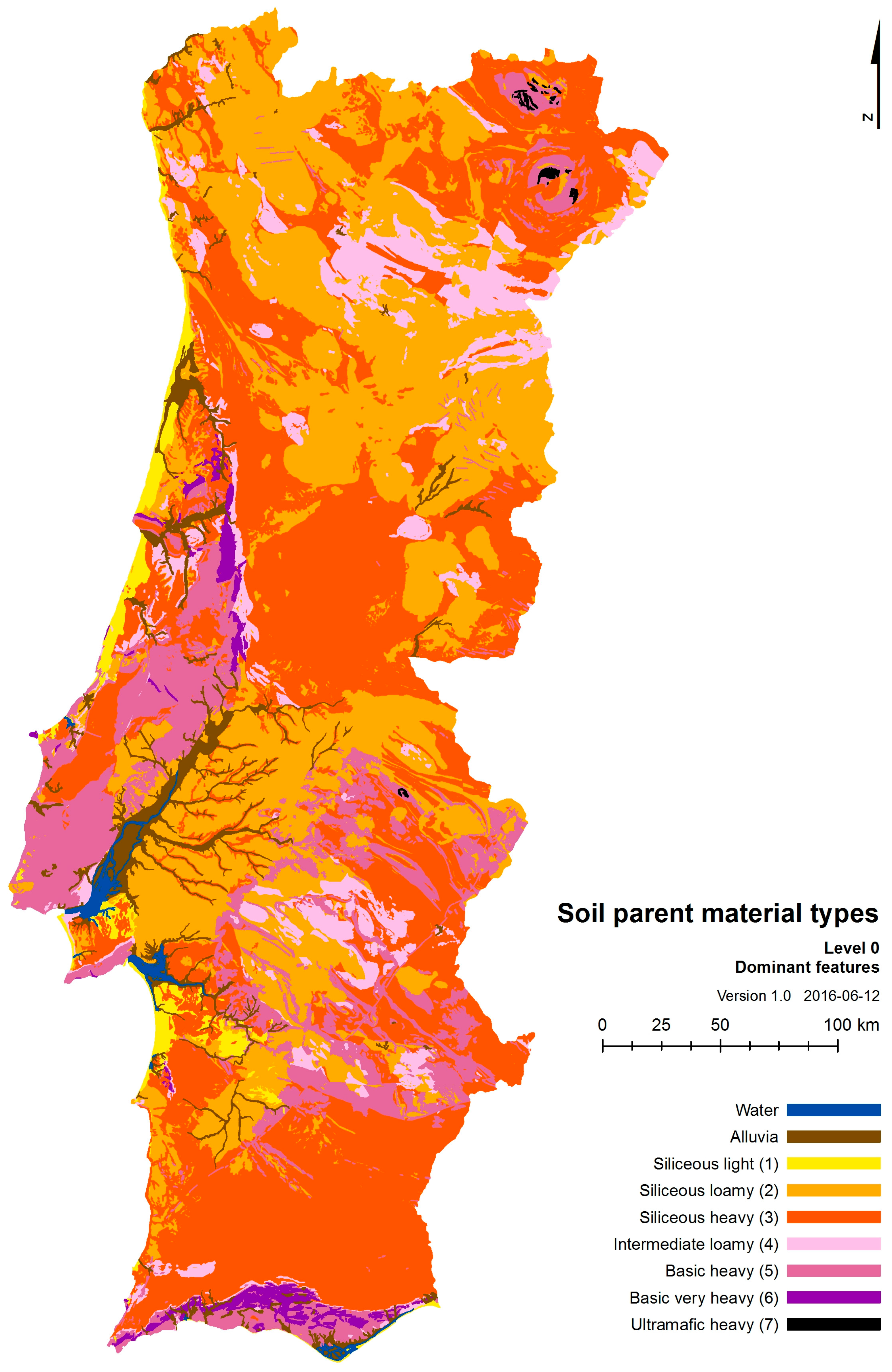
Soil parent material types (SPMType) were also tested as an edaphic explanatory variable, derived from the 1/500,000 Portuguese Geologic Map [77]. Appendix A details the methodology used to construct this variable; see also, in the same appendix, Table A1 and Table A2 where further information is given on the construction of SPMType and Figure A1 where a map of SPMType is presented.
Table 1 lists the 15 putative explanatory variables, the respective abbreviations, an informal classification of the variable type and the physical phenomenon related to each variable.
2.2. Data Pre-Treatments
Pearson correlation coefficient (r) among all variable pairs was checked and multicollinearity was further assessed calculating the variance inflation factors for each taxon dataset using function vif from R package usdm [78]. For all taxa datasets r among all possible pairs of variables used in models was lower than 0.7 (see Figures S8–S12 in Supplementary Materials.). Variance inflation factors were under 2.8 (9.0 excluding zero saplings) for Q. broteroi and under 2.9 (5.2 excluding zero saplings) for all other species, showing low multicollinearity levels. Tables S1–S5 in Supplementary Materials present summary statistics for all variables in all datasets.
The presence of spatial autocorrelation on saplings data was checked with the Mantel test and 10,000 Monte Carlo permutations using mantel.rtest function from package ade4 [79]. For all taxa, the simulated p-values were between 0.75 and 0.97, indicating no correlation between saplings data (excluding zero saplings) and the respective Euclidean distance matrices.
Extreme observations can bring additional ecological insight. However, it was not feasible to compare the fitting results with and without extreme observations, due to the long computation time of the fitting process. After inspecting saplings boxplots for each species, we decided to exclude a few clearly isolated data points corresponding to suspicious extremely high counts; Figure S13 in Supplementary Materials shows the boxplots produced and Table 2 indicates the number of extreme observations removed. Table 2 shows, additionally, which soil parent material types (SPMType) were tested for each taxon and the total number of plots used to implement the models for each taxon (i.e., the total number of plots with available information on both saplings and the 15 explanatory variables).
2.3. Zero-Inflated Count Data Models
Zero-inflated count data models (ZICDM) are two-component mixture models that extend the classical generalized linear models (GLM) to account for excess of zeros in the dataset. One component incorporates a point mass at zero while the other corresponds to a count distribution such as Poisson or negative binomial. Therefore, zeros might come both from the point mass and from the count component. ZICDM using a negative binomial count model include a dispersion parameter θ in the modelling procedure, enabling the incorporation of both the excess of zeros and over-dispersion [80].
Following Zeileis et al. [80] the regression equation for the mean of a ZICDM, using the canonical log link for the count component, can be written as:
where is the probability of belonging to the point mass component, that is, in our case, the probability that regeneration is absent (zero saplings). The second component is simply the conditional mean coming from the count model (as in a classical Poisson or negative binomial GLM). ’s correspond to the coefficients of the count model ( the intercept), which multiply by each of the selected explanatory variables ().
The unobserved probability is modelled, simultaneously, by a binomial GLM, which conditional mean can be written, using the standard logit link, as:
where ’s correspond to the coefficients of the zero inflation component ( the intercept), which multiply by each of the selected explanatory variables () [80].
The coefficients β and γ, as well as the dispersion parameter θ (for the negative binomial count model) can be estimated, simultaneously, by maximum likelihood [80,81,82]. ZICDM are particularly appropriate to model saplings count data coming from national forest inventories. As count data, saplings number is appropriately handled by the count component of the model (by using Poisson or negative binomial distributions). Additionally, it is plausible that some species do not regenerate in some regions due to, for example, environmental constraints (which ultimately result in the absence of that species in that regions); as a result, an excessive number of zeros occur in the data. However, in the regions where regeneration is more probable, plots presenting zero saplings can still occur (e.g., by a simple matter of chance); these zeros are modelled by the count component.
Interestingly, by combining a logistic response (zero inflation component) with an exponential response (count component), it is possible for ZICDM to fit unimodal responses for a variable (thus, not only monotonic, as logistic or exponential by their own, when using first-degree polynomial terms). Additionally, such combined responses can also be asymmetric/skewed in shape. This added flexibility is only achievable when the variable in question is included in both components of the ZICDM.
2.4. Model Fitting
All the 15 chosen variables were tested as predictors in the count component. Regarding the zero inflation component, however, we decided to test OMBRO, THERM, SeedAvail and SoilMoist (i.e., as predictors of the absence of saplings). Other variables such as FireFreq, GRAZI, UnderClear can completely hinder regeneration (e.g., through very high fire frequency or overgrazing) but extremes in FireFreq are very rare in the studied area, thus not expected to produce a true inflation of zeros, neither the number of grazed or managed plots justifies their testing as zero inflating variables. Inversely, climatic variables can impede regeneration over extensive areas, for example, low OMBRO values represent severe summer drought, which in southern Portugal is expected to completely preclude the regeneration of temperate species like Q. robur. Another variable able to produce zero inflation is SPMType (e.g., Q. suber is known to be calcifugous); however, as it is a categorical variable, to avoid numerical problems and perfect fittings we decided simply to remove from the analysis the classes of SPMType presenting less than 10 sapling occurrences, for Q. robur, Q. pyrenaica, Q. suber and Q. rotundifolia, and, exceptionally, 5 for Q. broteroi (as the number of sapling occurrences was considerably lower).
To sample the number of saplings, NFI5 used two different subplot sizes, depending on the species dominating the forest plot, respectively 200 m2 subplots in plots dominated by Q. suber or Q. rotundifolia and 50 m2 subplots for all other species. Consequently, the logarithm of the subplot area was used as an offset in all of the fitted models, ensuring that saplings density was correctly modelled.
To decide between the Poisson and negative binomial distribution we firstly looked at the mean and variance of the response variable and checked the Wald-tests of log(θ).
Model fitting was performed in R statistical software 3.2.0 [83] using packages stats, utils, parallel [83], vegan [84] and pscl [85]. After rescaling continuous independent variables to zero mean and unit variance using function decostand (vegan package), we used zeroinfl function (pscl package) to fit the models and function AIC from package stats to extract the Akaike Information Criteria (AIC) of each model.
As variables influence is expected to vary between taxa, we individually fitted models for each Quercus taxon. Even if we understand that the inclusion of interactions between variables could certainly improve the obtained models [13,38], including 2-way interactions would have raised the number of possible model formulas to an impracticable number. Therefore we opted to not include interaction terms, focusing only on the main terms importance. In this way, the 15 variables used for the count component of the model and the 4 variables selected for the zero inflation component were combined in all possible ways using function combn from utils package to produce 524,288 different model formulas for each taxon.
We performed two sequential runs. In the first run we used: (i) SeedAvail with 2-km neighbourhoods, as we hypothesized that local scale effects on seed availability would be stronger than regional effects, due to the limited seed dispersal range usually found in the Quercus genus [33,34]; (ii) DensPp and DensEg with 10-km neighbourhoods, as we supposed the wider scale would best capture forestry intensity effects on regeneration; (iii) SoilMoist weighted by OMBRO, as the gradient of summer precipitation is pronounced in mainland Portugal and is an important limiting variable for the survival of seedlings and saplings. Therefore, in a first run we fitted models for all possible combinations of:
- On the count component: G, N, GRAZI, UnderClear, SeedAvail (2 km), DensPp (10 km), DensEg (10 km), FireFreq, OMBRO, THERM, TRASP, SLOPE, SoilMoist (summer) and SPMType;
- On the zero inflation component: SoilMoist (summer), OMBRO, THERM and SeedAvail (10 km).
After fitting all models and sorting them by increasing AIC we checked if SeedAvail, DensPp and DensEg were selected amongst the best model (lower AIC), or on some of the alternative models (∆AIC < 2). In case one (or more) of those variables was extant in this set of best models, we studied if other neighbourhood size (or a combination of neighbourhood sizes) minimized AIC further. Finally, when AIC decreased by replacing the neighbourhood size(s), we performed a second run, again fitting all the 524,288 combinations but now using the neighbourhood(s) which decreased AIC. Simultaneously, we also checked for AIC changes by replacing SoilMoist (summer) by SoilMoist (annual), whenever this variable was present in the set of best models. In case the replacement produced a decrease in AIC, we used SoilMoist (annual) in the second run. Even if we wanted to sense the differences between the different neighbourhood sizes and SoilMoist weights, we must stress that we expected minimal changes in the model performance, as the changes in neighbourhood or weight produced, generally, highly correlated variables (see Figures S8–S12 in Supplementary Materials.).
2.5. Variables Importance Value
AIC difference to the best model was calculated for each of the fitted models (). As the relative likelihood is directly proportional to a simple calculation using the ’s (), Akaike weights () can be computed for each model as:
where is the total number of models.
Finally, variable importance values were obtained for each of the tested variables, summing the Akaike weights of all models containing the variable:
Besides variable importance, we found essential to inspect the signal of the effect (i.e., positive or negative), in order to discuss the results from an eco-physiological point of view. We examined the signal of the fitted coefficients in the following way: after ordering all models by their respective Akaike weight (), we selected the first j models that totalized 0.95 of summed and checked if each variable sign was positive or negative among those models. A variable signal was considered consistent when always positive or negative within the first j models.
3. Results
As expected, a large proportion of plots had zero saplings; moreover, saplings variance was systematically greater than the mean (Table 3). Therefore the negative binomial distribution was used and, inspecting the set of best models, the logarithm of the dispersion parameter log(θ) was always significant in the Wald-test for all taxa.
Neighbourhood sizes and SoilMoist weights producing lower AIC values varied among the studied taxa. Considering SeedAvail, 2-km neighbourhoods produced better models for Q. robur and Q. pyrenaica, yet for Q. broteroi and Q. rotundifolia higher values were chosen. For DensPp, 10-km produced lower AIC values for Q. robur and 2-km for Q. pyrenaica, while for DensEg, the 10-km neighbourhood was selected both for Q. broteroi and Q. suber. Table 4 summarizes best neighbourhoods results, as well as SoilMoist best weight (summer or annual ombrothermic index).
The number of models used to study variable signal consistency was quite different among taxa (Table 5), meaning that, for some of the studied taxa, Akaike weights were more concentrated within the first models with lower AIC, than for other taxa. Figures S14–S18 in Supplementary Materials show graphically, for each taxon, the sorted AIC of all models and the proportion of the first (sorted) models that summed up to 0.95 of Akaike weight.
Importance values based on Akaike weights (), both for the count and zero inflation components, allowed us to identify the most and the least relevant variables for the regeneration of each taxon. Table 6 presents the obtained importance values (values greater than 75% are in bold). On the side of each importance value the result of the signal consistency analysis is also presented: an up arrow indicates a consistent positive effect of the variable in the taxon regeneration; a down arrow indicates a consistent negative effect; if both arrows are present, signal was not consistent in the analysed models. Signals were consistent for all variables with importance values greater than 80%.
In order to allow the inspection of (the best) obtained fits, we present in Tables S6–S10 in Supplementary Materials the summary outputs of the best model (lower AIC) for each taxon.
4. Discussion
4.1. Zero Inflation Component
Importance values for the zero inflation components of all studied taxa were very high for climatic variables, particularly OMBRO and, to a less extent, THERM. This was expected, as mainland Portugal encompasses two distinct macrobioclimates, temperate in the NW and Mediterranean in the rest of the territory [59,88] and climate is known to determine species absence from entire regions [89]. However, species and/or regeneration can be missing from areas that are climatically suitable. In fact, seed availability (SeedAvail), at relatively much smaller scales (from 2 to 10 km), presented also very high importance values, showing that the presence of nearby adult trees is critical for regeneration to occur. SoilMoist was less relevant by far. Still, zero-sapling occurrences of Q. robur decreased towards higher summer moisture areas (i.e., the bottom of the hills and valleys in areas with rainier summers), which agrees with the species preference for deep, cool soils under temperate climate [25,90].
4.2. Count Component
As expected, variable importance values were much different among each taxon. Notwithstanding, local to regional seed availability (SeedAvail) resulted positively linked to higher sapling densities for all taxa except Q. suber; the importance of nearby seed sources in Iberian Quercus regeneration was also found relevant by Gómez-Aparicio et al. [91]. OMBRO was also relevant for all taxa and its selection on both count and zero inflation components (with the same signal) indicates the modelling of non-monotonic responses. We now highlight other important variables for each taxon.
4.2.1. Q. robur
Q. robur regeneration was dependent on forest structure, increasing with basal area (G). In fact Q. robur ability to regenerate under intermediate to low levels of light is well-known [92,93]. However, higher tree densities (N) showed an opposite effect, which can be related to regeneration failure in younger and denser forests, probably plantations, where very low light levels can end up hindering Q. robur regeneration [94,95]. Fire frequency (FireFreq) was particularly relevant at hindering Q. robur regeneration, which agrees with this species sensitivity to recurrent fires that can lead to its replacement by shrubland [45]. DensPp had a moderate positive effect on Q. robur sapling density. Fast-growing pine plantations have long been introduced in the Mediterranean countries assuming they would facilitate hardwoods in the long-term [96]. In Portugal, this strategy was mostly unsuccessful but some old growth pine stands in the centre and north of Portugal currently comprise a substantial Q. robur component. We believe this relates to the effect found for DensPp, alongside with greater awareness of this species value. Sapling density was lower in southern aspects (TRASP), where summer water deficit is likely to be higher (or more severe) than in less sun-exposed terrain aspects.
4.2.2. Q. pyrenaica
The negative response of regeneration to higher basal area (G) or denser forests (N) concurs with [41], who studied the regeneration patterns of Q. pyrenaica and linked it to shade-intolerant species. Q. pyrenaica regeneration particularly suffered with understory clearing (UnderClear) and, to a lesser extent, with grazing (GRAZI). Indeed, this species occupies northern mountains where human settlements are scattered but extensive livestock grazing is still practiced [18,56]. Northern mountains display the highest fire frequency in Portugal, due to intricate relationships between land use, climate and topography [20,97]; accordingly, FireFreq affected sapling density negatively, as it did for Q. robur. Soils with heavier textures and higher base content (SPMType) had a positive effect on sapling abundance, similarly to Plieninger et al. [11] findings. Q. pyrenaica stands on such clayish and base-rich soils are rare in Portugal and are mainly limited to the NE region, where very dense stands with high and rapid regeneration have been described [56].
Although Q. pyrenaica occurrence is linked to the transitional areas between temperate and Mediterranean macrobioclimates, thus enduring summer drought better than Q. robur, southern aspects (TRASP) had lower sapling densities, like Q. robur. Contrariwise, DensPp had a negative effect on Q. pyrenaica, which might be related to forest management actions (as shown also by UnderClear) and possibly to the additional pressure this species suffers from its use as firewood [98].
4.2.3. Q. broteroi
After SeedAvail, regeneration of Q. broteroi was chiefly negatively affected by the regional density of E. globulus stands (DensEg). Q. broteroi use for firewood is documented in the centre west of Portugal, where it comprises a considerable proportion of burned firewood [99]. E. globulus stands planted for pulp production are widespread in this region. This possibly explains the regeneration depression in these areas due to both forest management practices and the overuse of Q. broteroi for firewood.
4.2.4. Q. suber
Basal area (G) affected Q. suber regeneration positively, in agreement with other studies where a nursing effect of tree cover was reported [39,100]. It is striking to note that Q. suber was the only taxon for which saplings density did not increase with the density of stands dominated or co-dominated by Q. suber adult trees in the neighbourhood (SeedAvail). In fact, regeneration failure in the montado system is a well-known and well-studied phenomenon [11,101,102] and most Portuguese Q. suber stands appear in the form of such cultural systems [103].
Grazing (GRAZI) is a common component of the agro-silvo-pastoral montado system and was highly relevant in depressing Q. suber regeneration, in agreement with studies showing that the montado sustainability is threatened by overgrazing, among other factors [101,102,104,105]. Slope arose also as an important variable, with flat areas associated with a decrease in regeneration; interestingly, montados are usually associated with flat areas [106]. Additionally, steeper terrain is usually less accessible, being less prone to human disturbances, as referred by Maia et al. [107].
Another remarkable finding is that Q. suber regeneration was positively associated to E. globulus stands, which was unexpected but it is justifiable. On one hand, E. globulus currently occupies a great fraction of the most oceanic Q. suber potential area in Portugal [19,47]. On the other hand, in this central-western part of Portugal it is common to find Q. suber trees exploited for cork, mainly in marginal areas, as a source of extra income for landowners. High environmental suitability for Q. suber and its presence either as scattered individuals or small stands, might explain its denser regeneration in those E. globulus dominated regions.
Q. suber is known to prefer siliceous substrata [90]. Considering SPMType, its saplings occurred in more than 10 stands for “siliceous loamy” (34.3%), “siliceous heavy” (60.7%) and “basic” (5%) types. Stands on “basic” substrata are considerably less in number, clearly evidencing its preferences. Yet, the variable did not result important as expected. We believe that the 15 stands on “basic” substrata might mainly result from mapping generalization errors (recall base data was on a scale of 1:500,000; see Appendix A) or from sites located in rainy areas where soil characteristics might change due to leaching.
4.2.5. Q. rotundifolia
From all studied taxa, Q. rotundifolia is the one able to withstand higher summer drought [108]. Its aptitude to thrive under dry climates is documented [109,110]. In fact, it was the only Quercus for which the probability of zero saplings increased with summer climatic moisture (OMBRO). As for the other Quercus, this was compensated by OMBRO in the count component (thus producing a non-monotonic response, as the others); however, it reflects the fact that sapling presence is concentrated towards summer drier regions, which are extensive in the centre and south of Portugal [59].
Recent fire events (TSLFire) triggered Q. rotundifolia regeneration, most probably linked to resprouting. Notwithstanding, high Firefreq resulted also negative for Q. rotundifolia regeneration but less importantly than for the temperate sub-Mediterranean species.
As for Q. suber, Q. rotundifolia is also frequently found dominating the tree layer of the Portuguese montado system. Yet, it is also commonly observed dominating residual and marginal forests throughout the Mediterranean areas of mainland Portugal. In Spain, the agro-silvo-pastoral system similar to montado, the dehesa, is also associated with a regeneration failure of Q. rotundifolia [106]. Yet, grazing (GRAZI) did not result relevant in obstructing Q. rotundifolia regeneration, as it did for Q. suber. This is somehow puzzling, as a similar pattern would be expected. However, both species co-occur frequently in Portugal and herbivore preference for Q. suber is documented [111,112], which can shed some light on why grazing affected these species differently. Nevertheless, as with Q. suber, slope resulted equally very relevant, with flat areas (common in montados) having decreased regeneration.
4.3. Selected Neighbourhoods
For all taxa, the most important variable affecting regeneration was the density of conspecific trees, that is, the proxy of local to regional seed availability (SeedAvail), being determinant in modelling regeneration absence (producing excess of zeros) and with the exception of Q. suber, it was also positively linked to sapling abundance. Quercus spp. seeds are known to be recalcitrant, with viabilities usually shorter than one year [113]. Thus, Quercus do not form a seed bank and, as expected, the proximity of adult trees resulted relevant for regeneration. Although different neighbourhoods performed differently for SeedAvail, changing neighbourhoods did not produce relevant changes in models. Nevertheless, for the temperate species Q. robur and Q. pyrenaica, 2-km neighbourhoods performed better (confirming our initial hypothesis), while for the Mediterranean species Q. broteroi and Q. rotundifolia, respectively, 5-km and 10-km performed better. In the case of Q. broteroi the neighbourhood increase might relate with the low number of adult stands in the dataset. The neighbourhood increase in Q. rotundifolia might relate with the highly continuous and even occurrence of this species in the southeast of Portugal.
Concerning DensPp and DensEg (which reflect local to regional forestry intensity), the 10-km neighbourhoods performed better in Q. robur, Q. broteroi and Q. suber models, as initially hypothesized. For Q. pyrenaica the 2-km neighbourhood was the best performing one; in this case we believe the relatively simpler rural landscapes where this species generally occurs allows the smaller neighbourhood to capture forestry pressure more readily. SeedAvail, DensPp and DensEg different neighbourhood performance could be better clarified by further work.
5. Conclusions
Mediterranean taxa sapling abundance (Q. suber and Q. rotundifolia) increased on less accessible sites, reflecting the long lasting and widespread anthropization of such landscapes. Actually, Q. suber regeneration was particularly impeded by cultural practices, namely grazing.
P. pinaster and E. globulus plantations had a negative effect on less noble essences (Q. broteroi and Q. pyrenaica), which are selectively collected for firewood in their regions of occurrence. Results suggest the more valuable Q. robur and Q. suber saplings are selectively protected under plantations, especially the latter, which is kept for cork harvesting and is strictly protected by law.
Disturbance is a well-known trigger of regeneration as it creates site availability. From the set of chosen variables, FireFreq, TSLFire, UnderClear and GRAZI are vegetation disturbances known to be very frequent in the Portuguese context. Wildfires became very frequent in mainland Portugal since the 1970s. Fire triggered the regeneration of Q. rotundifolia (TSLFire), nonetheless, high FireFreq reduced the abundance of its saplings. FireFreq was particularly relevant in hampering the regeneration of temperate sub-Mediterranean taxa (Q. robur and Q. pyrenaica). Although Quercus species resprout after fire [114], frequent fires can exhaust belowground storage reserves precluding further resprouting and kill saplings that have not yet stored enough reserves for resprouting [115].
Pooled analyses, for example, Vayreda et al. [116], although relevant for the study of more general traits (e.g., pines vs. broadleaves), can mislead the importance and relevance of variables. Vayreda et al. [116] concluded that climate and even disturbances, were less relevant drivers of regeneration. In fact, climate cannot be expected to be much relevant in a pooled analysis, as Quercus spp. are ubiquitous in the Iberian Peninsula, thus pooling them is likely to result in a no-effect for climatic variables. In this study we showed that different disturbances, as well as climatic variables, can be important and their relevance changes from taxon to taxon. Eventually, sapling density, as well as sapling absence, showed strong correlation to climate, thus, climatic changes are expected to impact regeneration in the future.
In a nutshell, management actions aiming at improving native forests regeneration should consider fire control (Q. robur, Q. pyrenaica and Q. rotundifolia), thinning of existing forest plantations, for example, P. pinaster (Q. robur and Q. pyrenaica) and avoiding practices that eliminate the taxon, like understory clearing (Q. pyrenaica and Q. broteroi), firewood overexploitation (Q. broteroi) and overgrazing (Q. suber).
Supplementary Materials
The following are available online at https://www.mdpi.com/1999-4907/9/11/694/s1, Figure S1: Maps of the no. of plots dominated or co-dominated by Q. robur adult trees (SeedAvail) in predefined neighbourhoods. Black dots represent sites where Q. robur saplings were found, Figure S2: Maps of the no. of plots dominated or co-dominated by Q. pyrenaica adult trees (SeedAvail) in predefined neighbourhoods. Black dots represent sites where Q. pyrenaica saplings were found, Figure S3: Maps of the no. of plots dominated or co-dominated by Q. broteroi adult trees (SeedAvail) in predefined neighbourhoods. Black dots represent sites where Q. broteroi saplings were found, Figure S4: Maps of the no. of plots dominated or co-dominated by Q. suber adult trees (SeedAvail) in predefined neighbourhoods. Black dots represent sites where Q. suber saplings were found, Figure S5: Maps of the no. of plots dominated or co-dominated by Q. rotundifolia adult trees (SeedAvail) in predefined neighbourhoods. Black dots represent sites where Q. rotundifolia saplings were found, Figure S6: Maps of the no. of plots dominated or co-dominated by P. pinaster adult trees (DensPp) in predefined neighbourhoods, Figure S7: Maps of the no. of plots dominated or co-dominated by E. globulus adult trees (DensEg) in predefined neighbourhoods, Figure S8: Pearson correlation coefficients (represented as ellipses) between pairs of variables used in the Q. robur models (n = 4167) [117], Figure S9: Pearson correlation coefficients (represented as ellipses) between pairs of variables used in the Q. pyrenaica models (n = 4461) [117], Figure S10: Pearson correlation coefficients (represented as ellipses) between pairs of variables used in the Q. broteroi models (n = 4631) [117], Figure S11: Pearson correlation coefficients (represented as ellipses) between pairs of variables used in the Q. suber models (n = 4485) [117], Figure S12: Pearson correlation coefficients (represented as ellipses) between pairs of variables used in the Q. rotundifolia models (n = 4642) [117], Table S1: Summary statistics for the Q. robur dataset (n = 4167), Table S2: Summary statistics for the Q. pyrenaica dataset (n = 4461), Table S3: Summary statistics for the Q. broteroi dataset (n = 4631), Table S4: Summary statistics for the Q. suber dataset (n = 4485), Table S5: Summary statistics for the Q. rotundifolia dataset (n = 4642), Figure S13: Sapling counts boxplots for all datasets. Whiskers extend 1.5 times the interquartile range. Outside whiskers, circles indicate observations that were used in the analysis, while crosses those removed, Figure S14: Top: Sorted AIC of all 524 288 fitted models for Q. robur. Bottom: Sorted model Akaike weights, for Q. robur and the respective fraction of the first models, which sum up to 0.95 and 0.99 of Akaike weight, Figure S15: Top: Sorted AIC of all 524 288 fitted models for Q. pyrenaica. Bottom: Sorted model Akaike weights, for Q. pyrenaica and the respective fraction of the first models, which sum up to 0.95 and 0.99 of Akaike weight, Figure S16: Top: Sorted AIC of all 524 288 fitted models for Q. broteroi. Bottom: Sorted model Akaike weights, for Q. broteroi and the respective fraction of the first models, which sum up to 0.95 and 0.99 of Akaike weight, Figure S17: Top: Sorted AIC of all 524 288 fitted models for Q. suber. Bottom: Sorted model Akaike weights, for Q. suber and the respective fraction of the first models, which sum up to 0.95 and 0.99 of Akaike weight, Figure S18: Top: Sorted AIC of all 524 288 fitted models for Q. rotundifolia. Bottom: Sorted model Akaike weights, for Q. rotundifolia and the respective fraction of the first models, which sum up to 0.95 and 0.99 of Akaike weight, Table S6: Summary output of the best fitted model for Q. robur, Table S7: Summary output of the best fitted model for Q. pyrenaica, Table S8: Summary output of the best fitted model for Q. broteroi, Table S9: Summary output of the best fitted model for Q. suber, Table S10: Summary output of the best fitted model for Q. rotundifolia.
Author Contributions
P.M.F. and T.M.-H. conceptualized and designed the project. P.M.F. and T.M.-H. collected data. T.M.-H. analysed data. T.M.-H. and P.M.F. prepared and revised the manuscript.
Funding
This research was funded by project SUSTAINSYS–Environmental Sustainable Agro-Forestry Systems (NORTE-07-0124-FEDER-0000044), financed by the European Regional Development Fund (ERDF) through the North Operational Regional Programme (ON.2-QREN) and by national funds through Fundação para a Ciência e a Tecnologia (PIDDAC-FCT-MEC). This research was also funded by the Fundação para a Ciência e a Tecnologia (FCT) grant number UID/AGR/04033/2013 and POCI-01-0145-FEDER-006958 (CITAB-UTAD). T.M.H. was partially funded by a postdoctoral grant within project SUSTAINSYS. T.M.H. was also funded by the European Social Fund (POCH) and by National Funds (MCTES), through a Fundação para a Ciência e a Tecnologia postdoctoral fellowship (SFRH/BPD/115057/2016).
Acknowledgments
We thank Ken Burnham and Maria João Martins for methodological advice, Annalisa Bellu for language checking and two anonymous reviewers for fruitful comments.
Conflicts of Interest
The authors declare no conflict of interest. The funders had no role in the design of the study; in the collection, analyses, or interpretation of data; in the writing of the manuscript and in the decision to publish the results.
Appendix A
This appendix details how the variable SPMType (soil parent material types) was constructed.
The chemical composition and texture/grain size of the parent material influence pedogenesis and mostly determine soil richness and texture, which also strongly depend on other important factors such as climate, biota and so forth. Soil parent material types were obtained by reclassifying the Portuguese Geological Map 1:500,000 [77]. We reclassified each geological map unit (rock types and formations) into seven classes, crossing the associated potential soil base richness and potential soil texture (see Table A1). To position each rock type/formation in each of the seven classes we used information on the richness in SiO2, K and Ca and also information on texture/grain size of the parent material. Table A2 presents a detailed characterization of the seven used classes, namely presenting the relative content in SiO2, K and Ca of the parent material, the central (potential) soil texture (i.e., usually associated with that parent material) and finally the rock types/formations that were included in each class (mainly in view of the context of mainland Portugal geologic principal features).

Table A1.
Potential richness-textural classes used to classify soil parent material.
| Textural Classes | ||||
|---|---|---|---|---|
| Light (Sandy) | Loamy | Heavy (Silty or Clayish) | ||
| Base richness | Siliceous | siliceous light | siliceous loamy | siliceous heavy |
| Intermediate | intermediate loamy | |||
| Basic | basic heavy | |||
| Ultramafic | ultramafic heavy | |||
Table A2.
Detailed characterization of the defined classes: relative content of SiO2, K and Ca, central (potential) soil texture and included rock types/formations.
Table A2.
Detailed characterization of the defined classes: relative content of SiO2, K and Ca, central (potential) soil texture and included rock types/formations.
| Class | Relative Content in | Central Soil Texture | Rock Types/Formations | ||
|---|---|---|---|---|---|
| SiO2 | K | Ca | |||
| siliceous light | ++++ | - | - | very light (sandy) | Siliceous sand formations. |
| siliceous loamy | +++ | ++ | - | (light to) loamy | Chert (flint, radiolarite), siliceous/ferric sandstone, consolidated dunes, siliceous conglomerate, quartz syenite, quartz trachyte, acid tuff, granite, rhyolite, syenite, trachyte, siliceous gneiss, siliceous paragneiss, arkose, quartz, quartz monzonite, quartz latite, quartzite. |
| siliceous heavy | ++ | + | + | (loamy to) heavy | Siliceous schist, clayish conglomerate, greywacke, siliceous phyllite, clayish sandstone, turbidite, mica schist, clayish schist, slate, lydite rich metasediments, claystone, clay, mudstone (shale, argilite), metapelite, silt, silty phyllite, siltstone, ampelite, silty arkose, expansive clays. |
| intermediate loamy | + | - | ++ | (light to) loamy (to heavy) | Granodiorite, monzonite, latite, foid syenite, phonolite, tonalite, tonalitic gneiss, quartz monzodiorite, monzodiorite, siliceous schist/phyllite with carbonated or calc-silicate layers, calciturbidite, quartz diorite, diorite, quartz monzogabbro. |
| basic heavy | - | - | +++ | (loamy to) heavy | Carbonate sandstone, carbonate breccia/conglomerate, sandstone + marlstone, sandstone + limestone, andesite, quartz gabbro, monzogabbro, basaltic andesite, mafic lamprophyre, diabase/dolerite, gabbro, foid gabbro, basalt, tephrite, marlstone + sandstone, limestone + sandstone, amphibolite, limestone + marlstone, marble, limestone. |
| basic very heavy | - | - | +++ | very heavy | Marlstone + limestone, marlstone, dolomite rock. |
| ultramafic heavy | - - | - * | var. | heavy | Basanite (igneous), ultramafic lamprophyre, pyroxenite, serpentinite, peridotite, metaperidotite, dunite. |
Legend: + and - signs indicate relative richness; * generally poor but rare exceptions occur; var.: very variable content.
Igneous rocks were positioned mainly using data from QAPF diagrams (Quartz, Alkali feldspar, Plagioclase and Feldspathoid) and the TAS (Total Alkali vs. Silica) diagram [118,119] and other specific mineralogical information of each rock type/formation, gathered in geological and similar publications. Sedimentary and metamorphic rocks/formations were positioned following specific mineralogical information of the respective rock type/formation, gathered in geological and similar publications. For the present work, the “basic heavy” and “basic very heavy” classes of Table A2 were merged into one single class called “basic heavy”.
After the reclassification, the new map was entered into a Geographical Information System (GIS) and orthoimagery was used to improve the map accuracy. In particular, using esri arcmap 10.0 SP5 Spatial Adjustment tools (rubersheet method) the obtained polygons were adjusted to the Portuguese official boundary [120], a highly accurate dataset of the Portuguese border, as well as, adjusted to match natural boundaries when unequivocally recognized in the orthoimagery provided by ESRI (ESRI basemaps, 50 cm resolution otrthoimages from DGRF collected from 2004 to 2006). Several natural boundaries between geological units could be recognized and were very useful to improve the map georeferencing, for instance:
- (i)
- boundaries between granitoid rocks and metasediments were sometimes recognizable in the orthoimages and particularly valuable in the centre and north of mainland Portugal.
- (ii)
- in the south, the transition between limestone and metasediments was often distinguishable in the orthoimages.
- (iii)
- ultramafic rocks, which are known to affect greatly the vegetation cover, allowed to add some correction points in the north-east of mainland Portugal, using the shift to other basic rocks.
- (iv)
- alluvial plains have usually dendritic shapes, matched to the easily recognizable river networks; additionally, their limits are also identifiable straightforwardly in orthoimages, as they often produce clear-cut geomorphologic transitions to the surrounding hills. Therefore, almost all the patches corresponding to alluvial sediments produced several georeferencing correction points.
In total 9875 (circa 25% on the border, 75% inland) control points were used to improve spatial accuracy of the produced dataset. Adjustments were slight (most, up to 600 m) but significantly improved by the matching with natural shapes and with the Portuguese border, thus certainly contributing to overall accuracy of the dataset. This spatial adjustment is, in practice, not much relevant at the 1:500,000 scale (recall 600 m correspond to 1.2 mm in the printed map) but is of utmost importance if the researcher wants to cross the dataset with other data with high spatial accuracy (e.g., point data coming from global positioning devices), as it was performed in the present article.
Some geological formations are composed of intricate layers of very different types of rocks (sometimes very thick) that might point to different classes. In such cases, we kept such information by defining different levels of classes. Although it is difficult to determine which of those complex layers dominate in terms of outcropping matter, based mostly on geological literature, we produced a first level of information (Level 0) where only the dominant class is mentioned. In Level 1 we ascribed (when present) up to two classes to such complex formations (thus, including the co-dominant class). In Level 2 we ascribed all the occurring classes, preserving the original geological information. In the present work, we used Level 0 (dominant class only, see Figure A1). This information can be downloaded from: http://home.isa.utl.pt/~tmh/.
Figure A1.
Soil parent material types map. The map contains other two classes: “alluvia” which are not easily classifiable within any of the defined classes, as their chemical composition and texture vary and “water”, corresponding to rivers, estuaries, etc.
Figure A1.
Soil parent material types map. The map contains other two classes: “alluvia” which are not easily classifiable within any of the defined classes, as their chemical composition and texture vary and “water”, corresponding to rivers, estuaries, etc.

References
- Food and Agriculture Organization of the United Nations. Global Forest Resources Assessment 2010: Main Report; FAO Forestry Paper; Food and Agriculture Organization of the United Nations: Rome, Italy, 2010; ISBN 978-92-5-106654-6. [Google Scholar]
- Bongiorno, S.F. Land use and summer bird populations in northwestern galicia, Spain. Ibis 1982, 124, 1–20. [Google Scholar] [CrossRef]
- Kwok, H.K.; Corlett, R.T. The bird communities of a natural secondary forest and a Lophostemon confertus plantation in Hong Kong, South China. For. Ecol. Manag. 2000, 130, 227–234. [Google Scholar] [CrossRef]
- Barlow, J.; Mestre, L.A.M.; Gardner, T.A.; Peres, C.A. The value of primary, secondary and plantation forests for Amazonian birds. Biol. Conserv. 2007, 136, 212–231. [Google Scholar] [CrossRef]
- Farwig, N.; Sajita, N.; Böhning-Gaese, K. Conservation value of forest plantations for bird communities in western Kenya. For. Ecol. Manag. 2008, 255, 3885–3892. [Google Scholar] [CrossRef]
- Calviño-Cancela, M.; Rubido-Bará, M.; van Etten, E.J.B. Do eucalypt plantations provide habitat for native forest biodiversity? For. Ecol. Manag. 2012, 270, 153–162. [Google Scholar] [CrossRef]
- Calviño-Cancela, M. Effectiveness of eucalypt plantations as a surrogate habitat for birds. For. Ecol. Manag. 2013, 310, 692–699. [Google Scholar] [CrossRef]
- Pina, J.P. Breeding bird assemblages in eucalyptus plantations in Portugal. Ann. Zool. Fenn. 1989, 26, 287–290. [Google Scholar]
- Proença, V.M.; Pereira, H.M.; Guilherme, J.; Vicente, L. Plant and bird diversity in natural forests and in native and exotic plantations in NW Portugal. Acta Oecol. Int. J. Ecol. 2010, 36, 219–226. [Google Scholar] [CrossRef]
- Williams, M. Deforesting the Earth: From Prehistory to Global Crisis: An Abridgment; University of Chicago Press: Chicago, IL, USA, 2006; ISBN 0-226-89947-0. [Google Scholar]
- Plieninger, T.; Rolo, V.; Moreno, G. Large-scale patterns of Quercus ilex, Quercus suber and Quercus pyrenaica regeneration in central-western Spain. Ecosystems 2010, 13, 644–660. [Google Scholar] [CrossRef]
- Carnicer, J.; Coll, M.; Pons, X.; Ninyerola, M.; Vayreda, J.; Peñuelas, J. Large-scale recruitment limitation in Mediterranean pines: The role of Quercus ilex and forest successional advance as key regional drivers. Glob. Ecol. Biogeogr. 2014, 23, 371–384. [Google Scholar] [CrossRef]
- Benavides, R.; Escudero, A.; Coll, L.; Ferrandis, P.; Ogaya, R.; Gouriveau, F.; Penuelas, J.; Valladares, F. Recruitment patterns of four tree species along elevation gradients in Mediterranean mountains: Not only climate matters. For. Ecol. Manag. 2016, 360, 287–296. [Google Scholar] [CrossRef] [Green Version]
- Benito-Garzón, M.; Ruiz-Benito, P.; Zavala, M.A. Interspecific differences in tree growth and mortality responses to environmental drivers determine potential species distributional limits in Iberian forests. Glob. Ecol. Biogeogr. 2013, 22, 1141–1151. [Google Scholar] [CrossRef]
- Stevens-Rumann, C.S.; Kemp, K.B.; Higuera, P.E.; Harvey, B.J.; Rother, M.T.; Donato, D.C.; Morgan, P.; Veblen, T.T. Evidence for declining forest resilience to wildfires under climate change. Ecol. Lett. 2017. [Google Scholar] [CrossRef] [PubMed]
- Mather, A.S.; Pereira, J.M.C. Transição Florestal e Fogo em Portugal. In Incêndios Florestais em Portugal: Caracterização, Impactes e Prevenção; Pereira, J.S., Pereira, J.M.C., Rego, F.C., Silva, J.M.N., da Silva, T.P., Eds.; ISAPress: Lisboa, Portugal, 2006; pp. 257–282. [Google Scholar]
- Louro, G.; do Monteiro, M.L.; Constantino, L.; Tomé, M.; Rego, F. Evolução do material lenhoso de pinheiro-bravo e eucalipto. Silva Lusit. 2010, 18, 133–149. [Google Scholar]
- Moreira, F.; Rego, F.C.; Ferreira, P.G. Temporal (1958–1995) pattern of change in a cultural landscape of northwestern Portugal: Implications for fire occurrence. Landsc. Ecol. 2001, 16, 557–567. [Google Scholar] [CrossRef]
- Costa, A.; Madeira, M.; Santos Lima, J. Is cork oak (Quercus suber L.) woodland loss driven by eucalyptus plantation? A case-study in southwestern Portugal. IFor. Biogeosci. For. 2014, 7, 193–203. [Google Scholar] [CrossRef]
- Fernandes, P.M.; Loureiro, C.; Guiomar, N.; Pezzatti, G.B.; Manso, F.T.; Lopes, L. The dynamics and drivers of fuel and fire in the Portuguese public forest. J. Environ. Manag. 2014, 146, 373–382. [Google Scholar] [CrossRef] [PubMed] [Green Version]
- Nunes, M.C.S.; Vasconcelos, M.J.; Pereira, J.M.C.; Dasgupta, N.; Alldredge, R.J.; Rego, F.C. Land cover type and fire in Portugal: Do fires burn land cover selectively? Landsc. Ecol. 2005, 20, 661–673. [Google Scholar] [CrossRef]
- Watt, A.S. On the causes of failure of natural regeneration in British oakwoods. J. Ecol. 1919, 7, 173–203. [Google Scholar] [CrossRef]
- Buckley, D.S.; Sharik, T.L.; Isebrands, J.G. Regeneration of northern red oak: Positive and negative effects of competitor removal. Ecology 1998, 79, 65–78. [Google Scholar] [CrossRef]
- Carnicer, J.; Barbeta, A.; Sperlich, D.; Coll, M.; Peñuelas, J. Contrasting trait syndromes in angiosperms and conifers are associated with different responses of tree growth to temperature on a large scale. Front. Plant Sci. 2013, 4. [Google Scholar] [CrossRef] [PubMed] [Green Version]
- Čater, M.; Batič, F. Groundwater and light conditions as factors in the survival of pedunculate oak (Quercus Robur L.) Seedlings. Eur. J. For. Res. 2006, 125, 419–426. [Google Scholar] [CrossRef]
- Latham, R. Co-occurring tree species change rank in seedling performance with resources varied experimentally. Ecology 1992, 73, 2129–2144. [Google Scholar] [CrossRef]
- Bazzaz, F.; Miao, S. Successional status, seed size and responses of tree seedlings to CO2, light and nutrients. Ecology 1993, 74, 104–112. [Google Scholar] [CrossRef]
- Canham, C.; Finzi, A.; Pacala, S.; Burbank, D. Causes and consequences of resource heterogeneity in forests: Interspecific variation in light transmission by canopy trees. Can. J. For. Res. Rev. 1994, 24, 337–349. [Google Scholar] [CrossRef]
- Rodríguez-Calcerrada, J.; Pardos, J.A.; Gil, L.; Reich, P.B.; Aranda, I. Light response in seedlings of a temperate (Quercus petraea) and a sub-Mediterranean species (Quercus pyrenaica): Contrasting ecological strategies as potential keys to regeneration performance in mixed marginal populations. Plant Ecol. 2008, 195, 273–285. [Google Scholar] [CrossRef]
- Gómez-Aparicio, L.; Zamora, R.; Gómez, J.M.; Hódar, J.A.; Castro, J.; Baraza, E. Applying plant facilitation to forest restoration: A meta-analysis of the use of shrubs as nurse plants. Ecol. Appl. 2004, 14, 1128–1138. [Google Scholar] [CrossRef] [Green Version]
- Callaway, R. Effect of Shrubs on Recruitment of Quercus-Douglasii and Quercus-Lobata. Ecology 1992, 73, 2118–2128. [Google Scholar] [CrossRef]
- Smit, C.; den Ouden, J.; Diaz, M. Facilitation of Quercus ilex recruitment by shrubs in Mediterranean open woodlands. J. Veg. Sci. 2008, 19, 193–200. [Google Scholar] [CrossRef]
- Vander Wall, S.B. The evolutionary ecology of nut dispersal. Bot. Rev. 2001, 67, 74–117. [Google Scholar] [CrossRef]
- Gómez, J.M. Spatial patterns in long-distance dispersal of Quercus ilex acorns by jays in a heterogeneous landscape. Ecography 2003, 26, 573–584. [Google Scholar] [CrossRef]
- Tilghman, N. Impacts of white-tailed deer on forest regeneration in Northwestern Pennsylvania. J. Wildland Manag. 1989, 53, 524–532. [Google Scholar] [CrossRef]
- Hewitt, N.; Kellman, M. Tree seed dispersal among forest fragments: II. Dispersal abilities and biogeographical controls. J. Biogeogr. 2002, 29, 351–363. [Google Scholar] [CrossRef]
- Boiffin, J.; Aubin, I.; Munson, A.D. Ecological controls on post-fire vegetation assembly at multiple spatial scales in eastern North American boreal forests. J. Veg. Sci. 2015, 26, 360–372. [Google Scholar] [CrossRef]
- Coll, M.; Peñuelas, J.; Ninyerola, M.; Pons, X.; Carnicer, J. Multivariate effect gradients driving forest demographic responses in the Iberian Peninsula. For. Ecol. Manag. 2013, 303, 195–209. [Google Scholar] [CrossRef]
- Caldeira, M.C.; Ibáñez, I.; Nogueira, C.; Bugalho, M.N.; Lecomte, X.; Moreira, A.; Pereira, J.S. Direct and indirect effects of tree canopy facilitation in the recruitment of Mediterranean oaks. J. Appl. Ecol. 2014, 51, 349–358. [Google Scholar] [CrossRef] [Green Version]
- Busing, R.T. Canopy cover and tree regeneration in old-growth cove forests of the Appalachian Mountains. Vegetatio 1994, 115, 19–27. [Google Scholar]
- Camisón, Á.; Miguel, R.; Marcos, J.L.; Revilla, J.; Tardáguila, M.Á.; Hernández, D.; Lakicevic, M.; Jovellar, L.C.; Silla, F. Regeneration dynamics of Quercus pyrenaica Willd. in the Central System (Spain). For. Ecol. Manag. 2015, 343, 42–52. [Google Scholar] [CrossRef]
- Lorimer, C.; Chapman, J.; Lambert, W. Tall understorey vegetation as a factor in the poor development of oak seedlings beneath mature stands. J. Ecol. 1994, 82, 227–237. [Google Scholar] [CrossRef]
- Hannon, G.E.; Bradshaw, R.; Emborg, J. 6000 years of forest dynamics in Suserup Skov, a seminatural Danish woodland. Glob. Ecol. Biogeogr. 2000, 9, 101–114. [Google Scholar] [CrossRef]
- Pausas, J.C.; Llovet, J.; Rodrigo, A.; Vallejo, R. Are wildfires a disaster in the Mediterranean basin?—A review. Int. J. Wildland Fire 2008, 17, 713–723. [Google Scholar] [CrossRef]
- Carrión, Y.; Kaal, J.; Antonio Lopez-Saez, J.; Lopez-Merino, L.; Martinez Cortizas, A. Holocene vegetation changes in NW Iberia revealed by anthracological and palynological records from a colluvial soil. Holocene 2010, 20, 53–66. [Google Scholar] [CrossRef] [Green Version]
- Ellison, A.M.; Bank, M.S.; Clinton, B.D.; Colburn, E.A.; Elliott, K.; Ford, C.R.; Foster, D.R.; Kloeppel, B.D.; Knoepp, J.D.; Lovett, G.M.; et al. Loss of foundation species: Consequences for the structure and dynamics of forested ecosystems. Front. Ecol. Environ. 2005, 3, 479–486. [Google Scholar] [CrossRef]
- Capelo, J.; Mesquita, S.; Costa, J.C.; Ribeiro, S.; Arsénio, P.; Neto, C.; Monteiro-Henriques, T.; Aguiar, C.; Honrado, J.; Espírito-Santo, D.; et al. A methodological approach to potential vegetation modeling using GIS techniques and phytosociological expert-knowledge: Application to mainland Portugal. Phytocoenologia 2007, 37, 399–415. [Google Scholar] [CrossRef]
- Costa, J.C.; Neto, C.; Aguiar, C.; Capelo, J.; Espírito Santo, M.D.; Honrado, J.; Pinto-Gomes, C.; Monteiro-Henriques, T.; Sequeira, M.; Lousã, M.; et al. Vascular plant communities in Portugal (Continental, the Azores and Madeira). Glob. Geobot. 2012, 2, 1–180. [Google Scholar] [CrossRef]
- Costa, J.C.; Monteiro-Henriques, T.; Neto, C.; Arsénio, P.; Aguiar, C. The application of the habitats directive in Portugal. Fitosociologia 2007, 44, 23–28. [Google Scholar]
- Eira, J.; Pinho, J.; Santos, C.; Buxo, J.; Godinho Ferreira, P.; Uva, J.; Moreira, J. Global Forest Resources Assessment 2010-Country Report-Portugal; Food and Agriculture Organization: Rome, Italy, 2010. [Google Scholar]
- Svenning, J.-C. A review of natural vegetation openness in north-western Europe. Biol. Conserv. 2002, 104, 133–148. [Google Scholar] [CrossRef] [Green Version]
- Bradshaw, R.H.W.; Hannon, G.E.; Lister, A.M. A long-term perspective on ungulate-vegetation interactions. For. Ecol. Manag. 2003, 181, 267–280. [Google Scholar] [CrossRef]
- Mitchell, F.J.G. How open were European primeval forests? Hypothesis testing using palaeoecological data. J. Ecol. 2005, 93, 168–177. [Google Scholar] [CrossRef] [Green Version]
- Carrión, J.S.; Fernández, S.; González-Sampériz, P.; Gil-Romera, G.; Badal, E.; Carrión-Marco, Y.; López-Merino, L.; López-Sáez, J.A.; Fierro, E.; Burjachs, F. Expected trends and surprises in the Lateglacial and Holocene vegetation history of the Iberian Peninsula and Balearic Islands. Rev. Palaeobot. Palynol. 2010, 162, 458–475. [Google Scholar] [CrossRef] [Green Version]
- Direcção-Geral dos Recursos Florestais. Resultados do Inventário Florestal Nacional 2005/2006, 5a Revisão; Direcção-Geral dos Recursos Florestais: Lisboa, Portugal, 2007; p. 70. [Google Scholar]
- Aguiar, C. Flora e Vegetação da Serra de Nogueira e do Parque Natural de Montesinho. Ph.D. Thesis, Universidade Técnica de Lisboa-Instituto Superior de Agronomia, Universidade Técnica de Lisboa (TULisbon), Lisboa, Portugal, 2001. [Google Scholar]
- Monteiro-Henriques, T. Landscape and Phytosociology of the Paiva River’s Hydrographical Basin. Ph.D. Thesis, Instituto Superior de Agronomia, Universidade Técnica de Lisboa (TULisbon), Lisboa, Portugal, 2010. [Google Scholar]
- Hijmans, R.J. Raster: Geographic Data Analysis and Modeling (Version 2.3-40). Available online: http://CRAN.R-project.org/package=raster (accessed on 28 December 2015).
- Monteiro-Henriques, T.; Martins, M.J.; Cerdeira, J.O.; Silva, P.; Arsénio, P.; Silva, Á.; Bellu, A.; Costa, J.C. Bioclimatological mapping tackling uncertainty propagation: Application to mainland Portugal. Int. J. Climatol. 2016, 36, 400–411. [Google Scholar] [CrossRef]
- Gavilán, R. The use of climatic parameters and indices in vegetation distribution. A case study in the Spanish Sistema Central. Int. J. Biometeorol. 2005, 50, 111–120. [Google Scholar] [CrossRef] [PubMed]
- Jarvis, A.; Reuter, H.I.; Nelson, A.; Guevara, E. Hole-Filled SRTM for the Globe Version 4. Available online: http://www.cgiar-csi.org/data/srtm-90m-digital-elevation-database-v4-1 (accessed on 9 April 2014).
- Evans, J. Topographic Radiation Index-ArcScripts. Available online: http://arcscripts.esri.com/details.asp?dbid=12643 (accessed on 12 April 2016).
- Tarboton, D.G. A New method for the determination of flow directions and contributing areas in grid digital elevation models. Water Resour. Res. 1997, 33, 309–319. [Google Scholar] [CrossRef]
- Tarboton, D.G. TAUDEM: Terrain Analysis Using Digital Elevation Model (Version 5.0.6). Available online: http://hydrology.usu.edu/taudem/taudem5/downloads5.0.html (accessed on 1 December 2013).
- R Core Team. R: A Language and Environment for Statistical Computing; R Foundation for Statistical Computing: Vienna, Austria (Version 3.0.1). Available online: http://www.R-project.org/ (accessed on 1 December 2013).
- Sarkar, D. Lattice: Multivariate Data Visualization with R; Use R! Springer: New York, NY, USA, 2008; ISBN 978-0-387-75968-5. [Google Scholar]
- Simpson, G.L. Permute: Functions for Generating Restricted Permutations of Data (Version 0.7-0). Available online: http://CRAN.R-project.org/package=permute (accessed on 1 December 2013).
- R Core Team. Foreign: Read Data Stored by Minitab, S, SAS, SPSS, Stata, Systat, dBase, … (Version 0.8-55). Available online: http://CRAN.R-project.org/package=foreign (accessed on 1 December 2013).
- Hijmans, R.J. Raster: Geographic Data Analysis and Modeling (Version 2.1-49). Available online: http://CRAN.R-project.org/package=raster (accessed on 1 December 2013).
- Bivand, R.; Keitt, T.; Rowlingson, B. Rgdal: Bindings for the Geospatial Data Abstraction Library (Version 0.8-10). Available online: http://CRAN.R-project.org/package=rgdal (accessed on 1 December 2013).
- Pebesma, E.J.; Bivand, R.S. Classes and methods for spatial data in R. R News 2005, 5, 9–13. [Google Scholar]
- Bivand, R.S.; Pebesma, E.J.; Gomez-Rubio, V. Applied Spatial Data Analysis with R; Springer: New York, NY, USA, 2008. [Google Scholar]
- Nicolau, R. (Maria Rita Rodrigues Carmona Nicolau) Modelação e Mapeamento da Distribuição Espacial de Precipitação-Uma Aplicação a Portugal Continental. Ph.D. Thesis, Universidade Nova de Lisboa-Faculdade de Ciências e Tecnologia, Lisboa, Portugal, 2002. [Google Scholar]
- Gonzalo Jiménez, J. Diagnosis Fitoclimática de La España Peninsular: Hacia Un Modelo de Clasificación Funcional de La Vegetación Y de Los Ecosistemas Peninsulares Españoles, 1st ed.; Serie Técnica Naturaleza y Parques Nacionales; Organismo Autónomo de Parques nacionales, Ministerio de Medio Amiente y Medio Rural y Marino de España: Madrid, Spain, 2010; ISBN 978-84-8014-787-3. [Google Scholar]
- Hijmans, R.J.; Cameron, S.E.; Parra, J.L.; Jones, P.G.; Jarvis, A. Very high resolution interpolated climate surfaces for global land areas. Int. J. Climatol. 2005, 25, 1965–1978. [Google Scholar] [CrossRef] [Green Version]
- Hijmans, R.J.; Cameron, S.E.; Juan, L.P.; Jones, P.G.; Jarvis, A.; Richardson, K. Worldclim. Available online: http://www.worldclim.org/ (accessed on 31 May 2009).
- Serviços Geológicos de Portugal. Carta Geológica de Portugal na Escala 1:500 000; SGP: Lisboa, Portugal, 1992. [Google Scholar]
- Naimi, B. Usdm: Uncertainty Analysis for Species Distribution Models (Version 1.1-12). Available online: https://rdrr.io/cran/usdm/ (accessed on 25 February 2016).
- Chessel, D.; Dufour, A.B.; Thioulouse, J. The ade4 package—I: One-table methods. R News 2004, 4, 5–10. [Google Scholar]
- Zeileis, A.; Kleiber, C.; Jackman, S. Regression models for count data in R. J. Stat. Softw. 2008, 27. [Google Scholar] [CrossRef]
- Mullahy, J. Specification and testing of some modified count data models. J. Econ. 1986, 33, 341–365. [Google Scholar] [CrossRef]
- Lambert, D. Zero-Inflated Poisson Regression, with an Application to Defects in Manufacturing. Technometrics 1992, 34, 1–14. [Google Scholar] [CrossRef]
- R Core Team. R Core Team. R: A Language and Environment for Statistical Computing; R Foundation for Statistical Computing: Vienna, Austria (Version 3.2.0). Available online: http://www.R-project.org/ (accessed on 25 December 2015).
- Oksanen, J.; Blanchet, F.G.; Kindt, R.; Legendre, P.; Minchin, P.R.; O’Hara, R.B.; Simpson, G.L.; Solymos, P.; Stevens, M.H.H.; Wagner, H. Vegan: Community Ecology Package (Version 2.2-1). Available online: http://CRAN.R-project.org/package=vegan (accessed on 25 February 2016).
- Jackman, S. Pscl: Classes and Methods for R Developed in the Political Science Computational Laboratory (Version 1.4.9); Department of Political Science, Stanford University: Stanford, CA, USA, 2015. [Google Scholar]
- Burnham, K.P.; Anderson, D.R.; Burnham, K.P. Model Selection and Multimodel Inference: A Practical Information-Theoretic Approach, 2nd ed.; Springer: New York, NY, USA, 2002; ISBN 978-0-387-95364-9. [Google Scholar]
- Burnham, K.P.; Anderson, D.R.; Huyvaert, K.P. AIC model selection and multimodel inference in behavioral ecology: Some background, observations and comparisons. Behav. Ecol. Sociobiol. 2010, 65, 23–35. [Google Scholar] [CrossRef]
- Rivas-Martínez, S.; Rivas Sáenz, S.; Penas, Á. Worldwide bioclimatic classification system. Glob. Geobot. 2011, 1, 1–634. [Google Scholar] [CrossRef]
- Woodward, F.I.; Williams, B.G. Climate and plant distribution at global and local scales. Vegetatio 1987, 69, 189–197. [Google Scholar] [CrossRef]
- Franco, J. do Quercus L. In Flora iberica: Plantas Vasculares de la Península Ibérica e Islas Baleares; Castroviejo, S., Laínz, M., López González, G., Montserrat, P., Muñoz Garmendia, F., Paiva, J., Villar, L., Eds.; Real Jardín Botánico-Consejo Superior de Investigaciones Científicas: Madrid, Spain, 1990; Volume II, pp. 15–36. ISBN 84-00-07034-8. [Google Scholar]
- Gómez-Aparicio, L.; Zavala, M.A.; Bonet, F.J.; Zamora, R. Are pine plantations valid tools for restoring mediterranean forests? An assessment along abiotic and biotic gradients. Ecol. Appl. 2009, 19, 2124–2141. [Google Scholar] [CrossRef] [PubMed] [Green Version]
- Van Hees, A.F.M. Growth and morphology of pedunculate oak (Quercus robur L) and beech (Fagus sylvatica L) seedlings in relation to shading and drought. Ann. Sci. For. 1997, 54, 9–18. [Google Scholar] [CrossRef]
- Welander, N.T.; Ottosson, B. The influence of shading on growth and morphology in seedlings of Quercus robur L. and Fagus sylvatica L. For. Ecol. Manag. 1998, 107, 117–126. [Google Scholar] [CrossRef]
- Ziegenhagen, B.; Kausch, W. Productivity of young shaded oaks (Quercus robur L.) as corresponding to shoot morphology and leaf anatomy. For. Ecol. Manag. 1995, 72, 97–108. [Google Scholar] [CrossRef]
- Valladares, F.; Chico, J.M.; Aranda, I.; Balaguer, L.; Dizengremel, P.; Manrique, E.; Dreyer, E. The greater seedling high-light tolerance of Quercus robur over Fagus sylvatica is linked to a greater physiological plasticity. Trees Struct. Funct. 2002, 16, 395–403. [Google Scholar] [CrossRef]
- Pausas, J.G.; Blade, C.; Valdecantos, A.; Seva, J.P.; Fuentes, D.; Alloza, J.A.; Vilagrosa, A.; Bautista, S.; Cortina, J.; Vallejo, R. Pines and oaks in the restoration of Mediterranean landscapes of Spain: New perspectives for an old practice—A review. Plant Ecol. 2004, 171, 209–220. [Google Scholar] [CrossRef]
- Fernandes, P.M.; Loureiro, C.; Magalhães, M.; Ferreira, P.; Fernandes, M. Fuel age, weather and burn probability in Portugal. Int. J. Wildland Fire 2012, 21, 380–384. [Google Scholar] [CrossRef] [Green Version]
- Cerqueira, M.; Gomes, L.; Tarelho, L.; Pio, C. Formaldehyde and acetaldehyde emissions from residential wood combustion in Portugal. Atmos. Environ. 2013, 72, 171–176. [Google Scholar] [CrossRef]
- Gonçalves, C.; Alves, C.; Pio, C. Inventory of fine particulate organic compound emissions from residential wood combustion in Portugal. Atmos. Environ. 2012, 50, 297–306. [Google Scholar] [CrossRef]
- Tiscar-Oliver, P. Patterns of shrub diversity and tree regeneration across topographic and stand-structural gradients in a Mediterranean forest. For. Syst. 2015, 24, 11. [Google Scholar] [CrossRef] [Green Version]
- Bugalho, M.N.; Caldeira, M.C.; Pereira, J.S.; Aronson, J.; Pausas, J.G. Mediterranean cork oak savannas require human use to sustain biodiversity and ecosystem services. Front. Ecol. Environ. 2011, 9, 278–286. [Google Scholar] [CrossRef] [Green Version]
- Simões, M.P.; Belo, A.F.; Fernandes, M.; Madeira, M. Regeneration patterns of Quercus suber according to montado management systems. Agrofor. Syst. 2015, 1–9. [Google Scholar] [CrossRef] [Green Version]
- Capelo, J. Nemorum Transtaganae Descriptio: Sintaxonomia Numérica das Comunidades Florestais e Pré-florestais do Baixo Alentejo. Ph.D. Thesis, Universidade Técnica de Lisboa-Instituto Superior de Agronomia, Lisboa, Portugal, 2007. [Google Scholar]
- Plieninger, T. Compatibility of livestock grazing with stand regeneration in Mediterranean holm oak parklands. J. Nat. Conserv. 2007, 15, 1–9. [Google Scholar] [CrossRef]
- Pulido, F.; Garcia, E.; Obrador, J.J.; Moreno, G. Multiple pathways for tree regeneration in anthropogenic savannas: Incorporating biotic and abiotic drivers into management schemes. J. Appl. Ecol. 2010, 47, 1272–1281. [Google Scholar] [CrossRef]
- Pulido, F.J.; Diaz, M.; de Trucios, S.J.H. Size structure and regeneration of Spanish holm oak Quercus ilex forests and dehesas: Effects of agroforestry use on their long-term sustainability. For. Ecol. Manag. 2001, 146, 1–13. [Google Scholar] [CrossRef]
- Maia, P.; Keizer, J.; Vasques, A.; Abrantes, N.; Roxo, L.; Fernandes, P.; Ferreira, A.; Moreira, F. Post-fire plant diversity and abundance in pine and eucalypt stands in Portugal: Effects of biogeography, topography, forest type and post-fire management. For. Ecol. Manag. 2014, 334, 154–162. [Google Scholar] [CrossRef]
- Rivas-Martínez, S.; Sáenz Laín, C. Enumeración de los quercus de la península ibérica. Rivasgodaya 1991, 6, 101–110. [Google Scholar]
- Corcuera, L.; Camarero, J.J.; Gil-Pelegrín, E. Effects of a severe drought on Quercus ilex radial growth and xylem anatomy. Trees Struct. Funct. 2004, 18, 83–92. [Google Scholar] [CrossRef]
- Corcuera, L.; Notivol, E. Differences in photosynthetic activity might explain the large-scale shifts in pine recruitment in favour of oaks in continental Mediterranean climates. Forestry 2015, 88, 248–256. [Google Scholar] [CrossRef] [Green Version]
- Bugalho, M.N.; Milne, J.A.; Racey, P.A. The foraging ecology of red deer (Cervus elaphus) in a Mediterranean environment: Is a larger body size advantageous? J. Zool. 2001, 255, 285–289. [Google Scholar] [CrossRef]
- Bugalho, M.N.; Milne, J.A. The composition of the diet of red deer (Cervus elaphus) in a Mediterranean environment: A case of summer nutritional constraint? For. Ecol. Manag. 2003, 181, 23–29. [Google Scholar] [CrossRef]
- Pasquini, S.; Mizzau, M.; Petrussa, E.; Braidot, E.; Patui, S.; Gorian, F.; Lambardi, M.; Vianello, A. Seed storage in polyethylene bags of a recalcitrant species (Quercus ilex): Analysis of some bio-energetic and oxidative parameters. Acta Physiol. Plant. 2012, 34, 1963–1974. [Google Scholar] [CrossRef]
- Catry, F.X.; Pausas, J.G.; Moreira, F.; Fernandes, P.M.; Rego, F. Post-fire response variability in Mediterranean Basin tree species in Portugal. Int. J. Wildland Fire 2013, 22, 919–932. [Google Scholar] [CrossRef] [Green Version]
- Clarke, P.J.; Lawes, M.J.; Midgley, J.J.; Lamont, B.B.; Ojeda, F.; Burrows, G.E.; Enright, N.J.; Knox, K.J.E. Resprouting as a key functional trait: How buds, protection and resources drive persistence after fire. New Phytol. 2013, 197, 19–35. [Google Scholar] [CrossRef] [PubMed]
- Vayreda, J.; Gracia, M.; Martinez-Vilalta, J.; Retana, J. Patterns and drivers of regeneration of tree species in forests of peninsular Spain. J. Biogeogr. 2013, 40, 1252–1265. [Google Scholar] [CrossRef]
- Murdoch, D.; Chow, E.D. Ellipse: Functions for Drawing Ellipses and Ellipse-Like Confidence Regions (Version 0.3-8). Available online: http://CRAN.R-project.org/package=ellipse (accessed on 31 May 2013).
- Le Bas, M.; Streckeisen, L. The IUGS systematics of igneous rocks. J. Geol. Soc. Lond. 1991, 148, 825–833. [Google Scholar] [CrossRef] [Green Version]
- Le Maitre, R.W.; Streckeisen, A.; Zanettin, B.; Le Bas, M.J.; Bonin, B.; Bateman, P.; Bellieni, G.; Dudeck, A.; Efremova, S.; Keller, J.; et al. Igneous Rocks: A Classification and Glossary of Terms: Recommendations of the International Union of Geological Sciences, Subcommission on the Systematics of Igneous Rocks, 2nd ed.; Cambridge University Press: Cambridge, NY, USA, 2004; ISBN 978-0-521-61948-6. [Google Scholar]
- Direção-Geral do Território Carta Administrativa Oficial de Portugal-Versão 2011. Available online: http://www.dgterritorio.pt/cartografia_e_geodesia/cartografia/carta_administrativa_oficial_de_portugal__caop_/caop__download_/carta_administrativa_oficial_de_portugal___versao_2011/ (accessed on 26 September 2011).
Table 1.
List of putative explanatory variables of Quercus regeneration and their succinct characterization.
Table 1.
List of putative explanatory variables of Quercus regeneration and their succinct characterization.
| Abbreviation | Variable Name (Units or Levels) | Variable Type | Related Physical Phenomenon |
|---|---|---|---|
| G | Basal area (m2 ha−1). | Forest structure | Light/space availability (proxy). |
| N | Tree density, independently of the species (no. of trees per m2). | Forest structure | Light/space availability (proxy). |
| GRAZI | Evidence of grazing by domestic animals, that is, cattle, equine, sheep, goat or swine (“yes”, “no”). | Anthropic (animal husbandry) | Vegetation disturbance. |
| UnderClear | Evidence of bushes removal, that is, mechanical removal, prescribed fire, manual removal, etc. (“yes”, “no”). | Anthropic (management) | Vegetation disturbance/space availability. |
| SeedAvail | Density of plots with conspecific adult trees (no. of plots in a predefined neighbourhood). | Seed source | Local to regional seed availability/conspecific adult presence. |
| DensPp | Density of plots with adult P. pinaster trees (no. of plots in a predefined neighbourhood). | Anthropic (land-use) | Local to regional forestry intensity (P. pinaster). |
| DensEg | Density of plots with adult E. globulus trees (no. of plots in a predefined neighbourhood). | Anthropic (land-use) | Local to regional forestry intensity (E. globulus). |
| FireFreq | Fire frequency (no. of fires between 1975–2006). | Fire | Recurrent vegetation disturbance. |
| TSLFire | Time since last fire (“≤5 years”, “>5 years”). | Fire | Vegetation disturbance/space availability. |
| OMBRO | Summer quarter ombrothermic index (mm °C−1). | Climatic | Summer climatic moisture (proxy). |
| THERM | Compensated thermicity index (°C*10). | Climatic | Air temperature. |
| TRASP | Transformed aspect (0 to 1). | Physiographic | Relative solar radiation; also related to moisture, temperature and wind shelter (proxy). |
| SLOPE | Slope (drop/distance). | Physiographic | Soil deepness (proxy); accessibility (proxy). |
| SoilMoist | Logarithm of the contributing area weighted by OMBRO or AOI (mm °C−1). | Hydrologic/edaphic | Summer soil moisture/annual soil moisture (proxy). |
| SPMType | Soil parent material types (“alluvia”, “siliceous light”, “siliceous loamy”, “siliceous heavy”, “intermediate loamy”, “basic heavy”, “ultramafic heavy”). | Edaphic | Parent material base richness and potential soil texture. |
Table 2.
SPMType tested classes for each taxon and total no. of plots used in modelling.
| Taxa | No. of Removed Extreme Observations | SPMType Tested Classes 1 | Total No. of Plots Used in Modelling |
|---|---|---|---|
| Q. robur | 0 | 1, 2 | 4167 |
| Q. pyrenaica | 2 | 1, 2, 4 | 4461 |
| Q. broteroi | 1 | 1, 2, 3, 4 | 4631 |
| Q. suber | 3 | 1, 2, 4 | 4485 |
| Q. rotundifolia | 1 | 1, 2, 3, 4 | 4642 |
1 SPMType: 1 “siliceous loamy”, 2 “siliceous heavy”, 3 “intermediate loamy”, 4 “basic heavy”.
Table 3.
Percentage of zeros, mean and variance of sapling by taxon.
| Taxa | % Plots without Saplings | Excluding Plots without Saplings | Including Plots without Saplings | ||
|---|---|---|---|---|---|
| Saplings Mean | Saplings Variance | Saplings Mean | Saplings Variance | ||
| Q. robur | 96.0% | 4.7 | 35.5 | 0.2 | 2.3 |
| Q. pyrenaica | 96.8% | 7.8 | 113.3 | 0.3 | 5.5 |
| Q. broteroi | 99.3% | 2.0 | 2.0 | 0.01 | 0.04 |
| Q. suber | 94.6% | 3.1 | 15.5 | 0.2 | 1.3 |
| Q. rotundifolia | 95.2% | 8.2 | 128.8 | 0.4 | 9.3 |
Table 4.
Neighbourhood dimensions and soil moisture weight selected for final run; shown only when significant (p-value < 0.05) in the Wald-test in some of the best models of the final run.
Table 4.
Neighbourhood dimensions and soil moisture weight selected for final run; shown only when significant (p-value < 0.05) in the Wald-test in some of the best models of the final run.
| Taxa | SeedAvail (count) | DensPp (count) | DensEg (count) | SoilMoist (count) | SeedAvail (zero) | SoilMoist (zero) |
|---|---|---|---|---|---|---|
| Q. robur | 2 km | 10 km | - | - | 10 km | summer |
| Q. pyrenaica | 2 km | 2 km | - | - | 5 km | - |
| Q. broteroi | 5 km | - | 10 km | annual | 10 km | annual |
| Q. suber | - | - | 10 km | - | 2 km | - |
| Q. rotundifolia | 10 km | - | - | - | 2 km | - |
Table 5.
Number of models where coefficients signals were examined.
| Taxa | No. of Models |
|---|---|
| Q. robur | 5289 |
| Q. pyrenaica | 1275 |
| Q. broteroi | 16,249 |
| Q. suber | 4272 |
| Q. rotundifolia | 18,551 |
Table 6.
Variable importance values based on Akaike weights both for the count and zero inflation components and respective signal consistency.
Table 6.
Variable importance values based on Akaike weights both for the count and zero inflation components and respective signal consistency.
| Variable | Variable Importance Values (Based on Model Akaike Weights) | |||||
|---|---|---|---|---|---|---|
| Q. robur | Q. pyrenaica | Q. broteroi | Q. suber | Q. rotundifolia | ||
| Count component | G | 95.8% (↑) | 72.1% (↓) | 26.7% (↑↓) | 99.9% (↑) | 28.3% (↑↓°) |
| N | 86.0% (↓) | 63.1% (↓) | 66.6% (↑↓°) | 45.8% (↓) | 33.2% (↑↓°) | |
| GRAZI | 45.2% (↓) | 61.6% (↓) | 40.2% (↓) | 98.9% (↓) | 30.1% (↑°↓) | |
| UnderClear | 56.6% (↓) | 99.4% (↓) | 35.1% (↓) | 29.8% (↓) | 31.5% (↑) | |
| SeedAvail | 100.0% (↑) | 99.9% (↑) | 99.9% (↑) | 34.9% (↑) | 98.8% (↑) | |
| DensPp | 76.4% (↑) | 78.0% (↓) | 31.2% (↑↓) | 30.7% (↑) | 32.8% (↑↓°) | |
| DensEg | 29.3% (↑↓) | 41.5% (↓) | 81.8% (↓) | 92.5% (↑) | 28.1% (↑↓) | |
| FireFreq | 100.0% (↓) | 93.6% (↓) | 29.2% (↑↓) | 31.9% (↑) | 60.8% (↑°↓) | |
| TSLFire | 34.0% (↑) | 27.7% (↑↓) | 47.4% (↑°↓) | 27.9% (↑↓°) | 73.0% (↓) | |
| OMBRO | 93.8% (↓) | 99.5% (↓) | 75.8% (↑°↓) | 99.0% (↓) | 54.5% (↑↓°) | |
| THERM | 36.5% (↑°↓) | 29.9% (↑↓) | 73.9% (↑) | 29.0% (↑↓) | 62.0% (↑°↓) | |
| TRASP | 83.7% (↓) | 94.2% (↓) | 68.5% (↑↓°) | 40.9% (↓) | 63.6% (↓) | |
| SLOPE | 27.5% (↑°↓) | 33.1% (↓) | 35.6% (↑) | 100.0% (↑) | 100.0% (↑) | |
| SoilMoist | 48.6% (↑) | 28.6% (↑↓) | 69.4% (↑°↓) | 30.6% (↓) | 41.5% (↑) | |
| SPMType | 28.8% | 99.8% | 29.3% | 15.2% | 71.9% | |
| Zero inflation component | SeedAvail | 100.0% (↓) | 100.0% (↓) | 100.0% (↓) | 100.0% (↓) | 100.0% (↓) |
| OMBRO | 100.0% (↓) | 100.0% (↓) | 100.0% (↑°↓) | 99.8% (↓) | 96.7% (↑) | |
| THERM | 92.1% (↓) | 100.0% (↑) | 76.5% (↑°↓) | 39.1% (↓) | 67.2% (↑↓°) | |
| SoilMoist | 75.5% (↓) | 48.7% (↑) | 69.1% (↑°↓) | 30.4% (↓) | 57.4% (↓) | |
(↑) consistent positive signal; (↓) consistent negative signal; (↑↓) inconsistent signal. When only a smaller proportion (<25%) of models containing the variable contributed to signal inconsistency, the less frequent signal is indicated with ° on the right of the respective arrow.
© 2018 by the authors. Licensee MDPI, Basel, Switzerland. This article is an open access article distributed under the terms and conditions of the Creative Commons Attribution (CC BY) license (http://creativecommons.org/licenses/by/4.0/).
Share and Cite
MDPI and ACS Style
Monteiro-Henriques, T.; Fernandes, P.M. Regeneration of Native Forest Species in Mainland Portugal: Identifying Main Drivers. Forests 2018, 9, 694. https://doi.org/10.3390/f9110694
AMA Style
Monteiro-Henriques T, Fernandes PM. Regeneration of Native Forest Species in Mainland Portugal: Identifying Main Drivers. Forests. 2018; 9(11):694. https://doi.org/10.3390/f9110694
Chicago/Turabian StyleMonteiro-Henriques, Tiago, and Paulo M. Fernandes. 2018. "Regeneration of Native Forest Species in Mainland Portugal: Identifying Main Drivers" Forests 9, no. 11: 694. https://doi.org/10.3390/f9110694
Note that from the first issue of 2016, this journal uses article numbers instead of page numbers. See further details here.