Abstract
Crown size estimations are of vital importance in forest management practice. This paper presents nonlinear models that were developed for crown width prediction of Black pine (Pinus nigra Arn.) natural, pure, even-aged stands in Olympus Mountain, central Greece. Using a number of measured characteristics at tree and plot level from 66 sample plots as independent variables, an attempt was made to predict crown width accurately, initially based on Least Square Analysis. At the second stage, nonlinear mixed effect modeling was performed in order to increase the fitting ability of the proposed models and to deal with the lack of between observations independence error assumption. Based on the same form, a generalized crown width model was developed by including six main regressors, such as the diameter at breast height, the total height, the canopy base height, the basal area, the relative spacing index and the diameter to quadratic mean diameter ratio, while at the final stage, the same model was expanded to mixed-effect. The proposed models were evaluated against independent crown width sample observations that were also obtained from the study area. The results showed that the two types of mixed-effect models performed equally well and, therefore, we propose those for use in forestry practice. Furthermore, the exact contribution of each inherent variable in crown width allometry was evaluated, thus providing a framework to facilitate field measurements for forest management predictions.
1. Introduction
Crown size is defined as the horizontal space that is available for the display of leaves [1]. It forms the tree growing space, which is associated with the availability of all of the required supplies for the tree growth [2]. Therefore, crown size is a critical feature of any tree growing at stand or open conditions, particularly in mountain areas, where water limitations rarely occur. In forestry practice, crown size estimation is considered of vital importance because it is associated with many different factors of forest management concern, such as the photosynthetic capacity [3], stem volume [4], increment efficiency [5], tree competition [6,7], tree health and vigor [8], as well as carbon, water and energy exchange [9]. From an ecological point of view, crown size directly affects many of the understory flora and fauna components by regulating the amount of the penetrated sunlight and precipitation to the lowest layers, thus retaining the forest moisture [10]. In order to measure the dimensions of a crown, Gregoire and Valentine [11] suggested several approaches. In the current research, it was assumed that crown size at above-ground level depends mainly on the crown dimensions at different directions forming an approximately circular shape via vertical projection [12]. Hence, its mathematical expression involves crown width measurements, or the horizontal distance between the edges of each tree crown passing through the center of the trunk to at least two vertical directions.
Hemery et al. [3] have pointed out the importance of modeling crown width under a thinning regime for final crop spacing by linking the diameter at breast height and the crown width (crown diameter) with the available growing space. However, the increasing use of remote sensing techniques in forestry has generated a need for well-defined allometric relationships between the basic dendrometric parameters in order to perform accurate estimations of the standing wood volume. Popescu et al. [13] demonstrated that the crown width is a tree dimension that is possible to measure directly with a lidar photogrammetric technique, while Gering and May [14] inversed a simple linear model for crown width prediction in order to predict diameter at breast height from aerial photos or photogrammetric data. Therefore, the development of forest tree allometric statistical models would provide valuable tools in forest management decision making by allowing the prediction of the relevant stand attributes. Despite the importance of crown width modeling, a limited number of studies have been published to date in comparison to studies related to tree-height prediction. In crown width modeling, the typical variable that has been used as a regressor is the diameter at breast height (e.g., [3,12,15,16,17]), mainly due to the fact that this variable is included in almost all types of forest inventories and it is easy to measure it in the field. Incorporation of additional variables would improve the fitting ability of the candidate regression models; however, it would require additional sampling effort. From a practical point of view, therefore, it would be very useful to use any variable that could be easily measured in the field as an independent variable, such as the dominant height, instead of their mean values [18]. A possible disadvantage of using stand-level attributes as regressors is the assumption that stands with similar characteristics are described by similar linear or nonlinear models, which is not fully accurate [19].
In many cases, crown width modeling has been based on data that has been obtained from installed sample plots or even from repeated measurements along the same tree, which most often present a hierarchical nested structure, thus violating the assumption of between observations error independence [20]. Therefore, we applied non-linear mixed effect modeling in order to ensure the independency assumption by adding a plot-specific random-effect part along with a fixed part in each estimated parameter during the modeling process. Mixed-effect models of forest growth and yield have been recommended by several authors in the literature as an alternative solution to independency issues emanating from ordinary least squares application (e.g., [19,21,22,23,24,25,26,27,28]). As far as crown width modeling is concerned, application of the mixed-effect modeling approach has been more limited as yet (Sánchez-González et al. [23], Ducey [29], Fu et al. [30,31], Hao et al. [32], Yang and Huang [7] and Sharma et al. [33,34]). In most cases, the mixed-effect models were reported to have generated more accurate predictions than the fixed effect models, since the structural heterogeneity, at tree or at stand level, was reflected by the random-effect parameters. In any case, a subsample of observations would always be used for calibration, although this might be a disadvantage during the data analysis. However, in many cases, four to five observations would suffice for a reasonable accuracy of the mixed-modeling predictions [21].
Black pine (Pinus nigra Arn.) is an important commercial tree species in Greece that covers an area of 281,692 hectares. Its annual wood volume amounts to 13,892,819 m3, corresponding to 10% of the country’s total wood production [35]. Black pine geographically extends from the Iberian Peninsula to the Alps, Apennine Mountains, and the Balkan region, Asia Minor, Crimea and the USA and Canada. In Greece, Black pine is mainly located in the mountains of the continental country with some populations also extending to the islands of the North Aegean Sea. In Olympus Mountain, which has served as the study area for the research presented in the current article, the Black pine forest stands are, to a big extent, pure, even-aged and they are managed by the Hellenic Forest Service predominately for wood production. Black pine, in addition to its economic value, has the ability to grow in degraded ecosystems. This is the reason that Black pine has been widely used in afforestation of mountain areas [36]. The canopy of Black pine protects the vulnerable soils from erosion by creating a physical obstacle against erodibility factors, such as rain and wind and also by supplying material for the formation of a thick protective layer of pine litter [37]. Therefore, the prediction possibility of the required growing space of this species would support forest management decisions regarding afforestation. Furthermore, the development of crown width prediction models could facilitate standing volume estimations via remote sensing analysis and the establishment of the most appropriate silvicultural regimes in the framework of sustainable forest management.
In the context of our research, the main hypothesis was that the crown width-diameter allometry of Black pine (Pinus nigra Arn.) would be significantly influenced by a combination of basic tree- and stand-level parameters, such as diameter, basal area, stand density measures and tree characteristics. Furthermore, an additional hypothesis was that the generalized crown width-diameter models of Black pine would be more accurate than the single mixed ones. Therefore, the specific objectives of our research involved the following: (i) to develop a crown width prediction model of Black pine for use in Greece and other countries (ii) to evaluate the combinatorial effect of basic tree- and stand-level parameters along with random variables of mixed models on crown prediction and (iii) to compare different crown prediction strategies.
2. Materials and Methods
2.1. Data
The research reported in the current article was conducted over a two-year period in Olympus Mountain, Central Greece, where 66 non-permanent sample plots were installed, so as to measure a number of variables at tree and stand level (Figure 1). Measurements were carried out in a total of 3442 trees over an area of approximately 73,477 hectares that also included the Olympus National Park. The main forest species in the area is Black pine (Pinus nigra Arn.) and, to a lesser extent, the Macedonian fir (Abies borisii-regis Mattf.), intermingled with broadleaved species in some restricted locations. The climate is a typical sub-Mediterranean and the annual rainfall is about 715 mm. The geological substratum is mainly composed of limestones, granite outcrops and flysch. The elevation from the sea level in the established sample plots varied between 780 and 1520 m, with a mean value of 1148 m. Slope steepness ranged between 1.11% and 64.90%, and averaged at 36.51% from the horizontal level.
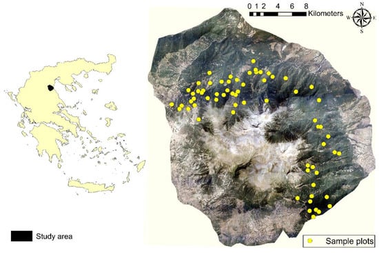
Figure 1.
Study area location map and distribution of the sample plots.
In order to select forest stands with Black pine as dominant species, a representative vector-format file (shapefile) of vegetation type and cover was used in GIS environment (ArcGIS 10.2, ESRI, Redlands, CA, USA) and 70 potential plot locations were selected randomly, using the random point function. Due to the complex terrain of the study area, the random sampling process made it possible to cover all the potential site qualities of the area. The shape of the sample plots was circular with stable radius, covering an area of 500 m2 in each case. In order to minimize the repeated measurements in each tree in an attempt to avoid the within-tree error correlation, we used the “canopy spread” module of LaserAce hypsometer (Trimble, Sunnyvale, CA, USA) to estimate the crown width (CW) in two vertical directions [38]. The diameter at breast height (DBH) was measured using a digital caliper to the nearest 0.1 m, and the total height (H) of each tree was measured by using the three-point measurement of LaserAce hypsometer. At stand level, the total basal area per hectare (BA in m2·ha−1), the number of stems per hectare (N·ha−1), the dominant height (mean height of the 100 largest trees per hectare or equally proportional—HDOM), the dominant diameter (mean diameter of the 100 largest trees per hectare or equally proportional—DDOM) and the quadratic mean diameter (QMD) were calculated. The HDOM and the DDOM were measured locally by selecting the five largest trees in each plot [39].
The Site Index in each plot was estimated using the Site Index Curves for Black Pine in Greece [40]. The total sample was composed of 3442 trees, the majority of which 90% was used for model development and about 10% for model validation [41]. The descriptive statistics of the total sample are shown in Table 1.

Table 1.
Descriptive statistics of the total sample.
2.2. Model Development
Diameter at breast height (DBH) is the most commonly used independent variable in crown width modeling, since the relationship between DBH and crown width (CW) has been well established in the literature. The mathematical form that links DBH and CW could be either linear [12,14,16,42] or nonlinear [7,23,30,34]. For the needs of the current research, a number of candidate simple linear and nonlinear models were fitted and the best ones, in terms of their fitting ability, were selected for further analysis. The candidate models are shown in Table 2.
Table 2.
Simple linear and nonlinear models for crown width modeling.
2.3. Additional Variables for Prediction-A Generalized Crown Width Model
It has been well established that DBH and CW for open and stand grown trees are closely correlated [44]. The incorporation of DBH as the only predictive variable assumes that trees of the same stem diameter also have the same mean crown dimensions, regardless of the competition levels inside the stand; an assumption that does not hold. In order to relax this assumption, previous research efforts have instead used tree variables, such as the crown length or ratio, the tree height and the distance dependent or independent stand-level predictors, which reflect the competition status [7,15,23,34,45]. The inclusion of additional variables leads to the creation of generalized models, which usually improve the crown width predictability in large areas under different stand competition regimes. However, a potential disadvantage of the generalized crown width prediction models is the inherent assumption that stands with similar attributes also present similar trends in crown modeling.
The inclusion of a number of stand attributes in the base model, which affect crown size, constitutes a standard procedure for expanding a simple model to a generalized form. For the sake of model simplicity, a number of predictors at stand level were tested [31] and the final form of the model was created. In this context, tree attributes, such as the total height (H), the height/diameter ratio (HDR) and the canopy base height (CBH), were used as covariates for crown width prediction. Furthermore, one tree-centered competition variable that is the basal area of the largest trees (BAL) and three size ratios, the diameter/dominant-diameter (DBH/DDOM), the height/dominant height (H/HDOM) and the diameter/quadratic mean diameter (DQMD), were tested in order to explain a larger part of crown variation. The most common distance-independent predictors at stand level that have been incorporated in generalized crown width models were the dominant height or diameter, the number of stems per hectare, the basal area, the quadratic mean diameter and the Reineke’s Stand Density Index (SDI), which was expressed as SDI = (N per ha) × (QMD/25.4)1.605 [46]. In the current research, in addition to the aforementioned stand level variables, the Relative Spacing Index (RSI), estimated as [34,47,48], was also evaluated during the development stage of a generalized nonlinear crown prediction model following a methodology which involved a direct addition of a variable into the model [33], thus approximating a forward selection method. The relationships of crown width with the basic variables at tree- and at stand- level are presented in the corresponding scatter plots (Figure 2). The candidate models were evaluated against each other using the ANOVA function for nested models in R statistical language (R Core Team) by using the Akaike information criterion (AIC), together with the log-likelihood (−2LL) ratio test and the statistical significance of each associated parameter.
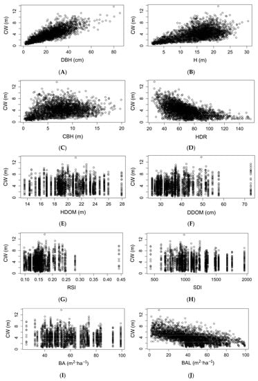
Figure 2.
Scatter plots of crown width against basic parameters at tree and stand level of the fitting data. DBH = diameter at breast height, H = total height, CBH = canopy base height, HDR = height/diameter ratio, HDOM = height of the 100 largest trees per hectare or equally proportional, DDOM = diameter of the 100 largest trees per hectare or equally proportional, RSI = relative spacing index, SDI = Reineke’s stand density index, BA = basal area, BAL = basal area of the largest trees. (A) diameter at breast height versus crown width (B) total height versus crown width (C) canopy base height versus crown width (D) height/diameter ratio versus crown width (E) dominant height versus crown width (F) dominant diameter versus crown width (G) relative spacing index versus crown width (H) Reineke’s stand density index versus crown width (I) basal area versus crown width (J) basal area of large trees versus crown width.
2.4. Mixed Effect Models
Very often, the field measurements that are obtained from established sample plots present a hierarchical nested structure, which violates the basic least square assumption of between observations independence [32]. The mixed effect models provide an appropriate framework to overcome this limitation [49] by estimating plot average parameters along with a random part, which is related specifically to each sample plot and, consequently, to the stand average conditions. The general vector form of a mixed effect model, with respect to crown width modeling, was expressed as:
where CWi was a vector of crown widths for the ith plot, f was a nonlinear function, Φi was a parameter vector, with r to represent the total number of the fixed effects in the model, DBHi was the predictor vector for ni observations and ei was the vector of the residuals. The Φi vector consisted of one fixed effect part which was the same for the entire population and a random effect part which was unique for each plot [20]. The vector of random effects and the error vector were assumed to be uncorrelated and normally distributed with zero mean and variance-covariance matrices D and Ri, respectively [7,27]. The Ri variance-covariance matrix was expressed as [50]:
where σ2 was a scaling factor for error dispersion [49], Gi was the diagonal matrix for within plot variance heteroscedasticity and Γi was an identity matrix that was related to the within plot autocorrelation structure of the residuals. When evidences of heteroscedasticity are present, a variance function may be applied, such as the power, the exponential and the constant/power functions [20,30,34,51], so as to link variance with a predictor. The diagonal elements of G matrix are provided by the selected variance function. Assuming that the i indicator represents the different plots and the j indicator represents each tree located within the plot, the variance functions were expressed through the following mathematical expressions [31]:
where δ, δ1 and δ2 are parameters to be estimated. The most suitable function was determined by visual inspection of the residuals and the Akaike Criterion (AIC).
2.5. Statistical Analysis
In order to evaluate the fitting ability of the ordinary least square and the mixed effect models, the following criteria were selected:
- the root mean square error (RMSE)
- an efficiency index (EI) based on R-squared expression [28]:
- the Akaike Information Criterion (AIC):AIC=−2log(L)+2p
- the mean prediction bias:where CWj, και represent the measured, estimated and mean values of crown width of the jth observation, n the total number of observations, p the number of the estimated model parameters and L the log-likelihood function of the fitted model. In addition, the model parameter estimates should be statistically different from zero. Visual inspection of the residuals was used, so as to detect heteroscedasticity trends. Following the suggestions of Temesgen et al. [52], the threshold value of bias was set to 10cm in order to preclude severely biased equations.
2.6. Calibrated Response
In general, the fitting procedure of crown width modeling requires a minimum number of observations to produce unbiased estimates at stand level. The corresponding required number of observations for height-diameter model fitting should be at least 20–25 per stand, according to van Laar and Akça [53]. An interesting property of mixed models is the ability to calibrate the random part of the parameters, even if a small number of observations would be available, and still obtain sufficiently accurate estimates. Usually four to five observations per stand would be sufficient enough to calibrate a mixed model and to obtain reliable parameter estimates [21,30]. In our case, the random effects vector prediction was based on the following Bayesian estimator [54]:
where was the estimated variance-covariance matrix for the random parameters, the variance-covariance matrix for within plot variability, was the matrix of partial derivatives, estimated at , with respect to its fixed parameters [21]. Using the derivatives of Equation (11) for a total sample of j = 2 trees from ith plot, the matrix becomes []. The algorithm was suitably implemented in R statistical language along with the nlme function.
The performance of each Black pine crown width model, generalized or mixed, was further evaluated against independent Black pine validation data, which were not included in model development. Two main sample scenarios were formulated in an effort to assess the predictive ability of each modeling technique separately:
- No calibration, use of only fixed effect parameters.
- Four observations of crown width-diameter [34].
The procedure was repeated 100 times for each plot, following different combinations of randomly selected trees [28]. The mean values of the statistical measures after 100 repetitions were reported for comparison.
The evaluation was based on the mean values of RMSE and bias, which were obtained through the fitting process of the proposed models in each of the six validation sample plots. The analysis was based on R statistical language, the nls function for nonlinear modeling and the nlme function for nonlinear mixed effect models.
3. Results
3.1. A Simple Mixed Effect Model
The fitting statistics of the simple least square nonlinear models are presented in Table 3.
Table 3.
Fitting statistics of the simple models
All the parameter estimates were statistically significant at (p < 0.01) level. All models, except the M4 model, predicted crown width relatively well, although the linear M1 and the nonlinear M2 appeared more accurate during the calibration stage. Based on the fitting statistics of Table 3, the M2 model performed slightly better than the M1 and, therefore, it was selected as the basis for mixed effect development. At the first stage, it was assumed that both the M2 fixed parameters contained a random part [55], according to the following form (MM1):
where b0 and b1 were the random effects of the model. The model converged at the calibration stage, however we detected evidence of heteroscedasticity in the residual plots. In order to minimize the unequal variance trends, the variance was modeled with functions, which were compared in terms of their fitting performance.
According to the results presented in Table 4, the constant-power function provided significantly different results compared to the same model using equal residual variance. The parameter estimates and fit statistics of the final model are presented in Table 5. In order to examine the coverage extent of the mixed model on both the fitting and the validation data, the mixed model was localized for each plot by using four randomly selected trees (Figure 3). According to Figure 3, the simple mixed model covered the range of the observed crown width values of the total sample.
Table 4.
Fitting statistics of the simple mixed model (MM1), using different types of variance functions.
Table 5.
Estimated parameters and fitting statistics of the simple mixed model (MM2).
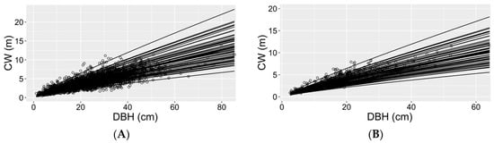
Figure 3.
Localized curves of simple mixed model (MM2) based on four randomly selected trees overlaid on the fitting data (A) and on validation data (B).
Hence, the final form of the simple mixed-effect model was
MM1 + constant-power function MM2
All the estimated parameters were significantly different than zero, according to the t-statistic test values.
3.2. Development of a Generalized Model
The following model form (13) presented the best fitting ability and it was selected as a generalized model for the prediction of black pine crown width. Using a total number of six predictors, it can be expressed as (GM1):
The residual analysis of the GM1 model revealed trends of unequal variance (heteroscedasticity), since variance changed as diameter values were increasing. Following the methodology described by Ritz and Streibig [56], a weighted least square method was used with weights in form of a function. The power function yielded the best results, and the final form of the proposed ordinary least square model is presented in Table 6.
Table 6.
Estimated parameters and fitting statistics of GM2.
Hence, the final form of the generalized model was
GM1 + power function GM2
The fixed parameters of the GM2 model were statistically significant at the p < 0.001 level.
The contribution of each covariate of the GM1 model to the variations of crown width is presented in Figure 4. The curves were created by using the mean values of the variables in Table 1, the fixed parameters of Table 6 and equal intervals of the test variable, starting from the minimum to the maximum range [33,34].
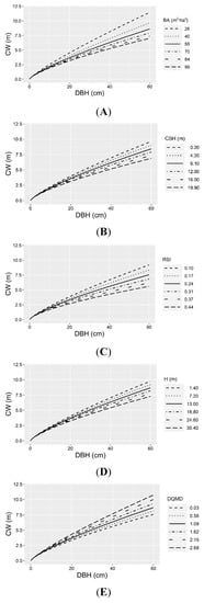
Figure 4.
Effects of the GM2 model’s covariates ((A) BA, (B) CBH, (C) RSI, (D) H, and (E) the diameter/quadratic mean diameter, DQMD) on the crown width of Black pine.
3.3. Development of a Generalized Mixed Effect Model
Starting from the mathematical form of the GM1 model, it was assumed that both fixed parameters, that is β0 and β1, contain a random part and that the model converged for the fitting data. However, the random part of the β1 parameter revealed almost zero variation and the model was simplified by modifying the β1 parameter to fixed. In addition, the parameter estimate (β6) that was linked to DQMD was not significant according to the t-statistic criterion and the mixed model was precluded from further analysis. The GM1 model was further modified by excluding the DQMD variable and convergence was achieved with both two and one random parameters. The two nested models were compared between them with the ANOVA method [20] and no significant differences were detected between them following the results of the log-likelihood ratio test (−2LL) (p > 0.05). This resulted in the selection of the simplest form of the two models with one random variable, according to the following mathematical expression (GMM1):
The residual analysis of the GMM1 model revealed treads of unequal variance and a constant-power function was used to model variance with diameter. The final form of the proposed generalized mixed model was (GMM2):
GMM1 + constant-power function GMM2
The parameter estimates and fit statistics of the proposed generalized mixed model are presented in Table 7. The fixed parameters of the GMM2 model were significant at the p < 0.001 level.
Table 7.
Estimated parameters and fitting statistics of the GMM2.
The extent of GMM2 coverage to crown width variation of the total sample was tested graphically by localizing the mixed-effect parameters to each sample plot using a random sample of four trees. According to Figure 5, the generalized mixed effect model covered the largest part of crown variation.
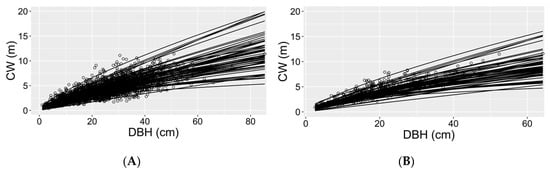
Figure 5.
Localized curves of the generalized mixed model (GMM2) based on four randomly selected trees overlaid on the fitting data (A) and on validation data (B).
In an effort to compare the two modeling strategies (simple and generalized mixed modelling), the distribution of the standardized residuals was evaluated graphically (Figure 6).
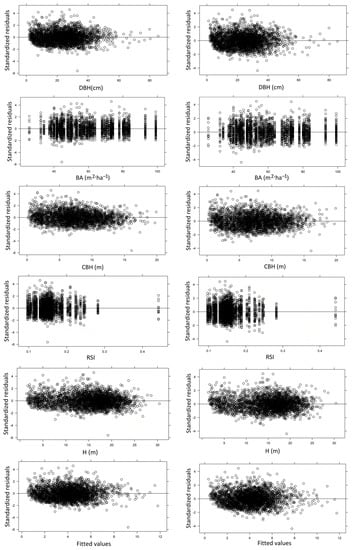
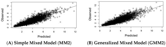
Figure 6.
Comparison of the two modelling strategies, simple mixed model (A) and generalized mixed model (B).
According to Figure 6, the two models performed equally well, with slightly better fitting of the GMM2 model. However, both models revealed no trends of unequal variance across the total range of the tested variables.
3.4. Evaluation
A total set of n = 362 trees from six randomly selected independent plots that were located at different stands within the study area was used in order to evaluate the predictive ability of the simple mixed (MM2) and the generalized mixed (GMM2) models. The fixed-effect (FE) corresponded to the fixed-effect part of the corresponding model.
The value attributes of the independent sample were among those that were used for model development, while the calibration of the mixed model random parameters was based on the random selection of four trees.
After a series of combinations of random tree selection, the mean RMSE values of all the modeling techniques were calculated, and they are presented in Figure 7. As it is shown in Figure 7, it can be concluded that both mixed models (MM2 and GMM2), for which a pre-sample for calibration of four random trees was used, could predict crown width with low RMSE, when compared to fixed models. The RMSE for all six sample plots was 0.966 m and the mean bias was 0.0021 m for the MM2 model, while the corresponding values for GMM2 were 0.933 m and 0.2557 m, respectively.
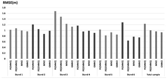
Figure 7.
Root mean square error values per sample plot and total sample during model evaluation against independent data of crown width-diameter. FE = fixed-effect part of the corresponding model in the parenthesis.
The corresponding mean value as the minimum possible RMSE from the simple least square analysis for each separate plot was 0.782 m for the basic model and 0.994 m for GM2, whereas the fixed parts (FE) of the mixed models presented the highest RMSE, that is, 1.232 m for MM2 and 1005 m for GMM2. The mean bias of the generalized model (GM2) was about 0.445 m which is relevant to under prediction biases of crown width.
4. Discussion
The models presented in the current article explained the greatest part of the crown width variation, a finding that has also been pointed out by other relevant studies [33,34]. The crown width-diameter allometry tends to be explained by a linear model, despite the slightly better performance of the M2 model, which complies with the findings of Dawkins [42]. However, the power-type M2 model was considered as more flexible since it was easy to be linearized and then expanded to a mixed effect model. The same model for crown width modeling has also been used by Russell and Weiskittel [57] and Sharma et al. [33,34]. In its simple form, the stem diameter is the only predictor of crown horizontal dimension, which is not as accurate because such models seem to overestimate crown size for dense stands and to underestimate it for sparse stands [33,58]. Indeed, as it is shown in Figure 7 and Figure 8, the simple model that only uses DBH as the independent variable, that is the FE (MM2) model, presented the largest error values along with the most biased estimates of all models that were tested. For this reason, a number of covariates at tree and at stand level were added to increase the percentage of crown variation that could be explained by the model.
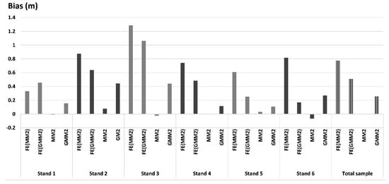
Figure 8.
Mean prediction bias per sample plot and total sample during model evaluation against independent data of crown width-diameter.
Basal area, as a measure of stand density, is expected to affect crown width [59], while the canopy base height has been mentioned as a valid predictor of crown width by a number of relevant studies [31,32,33,34]. Tree height has also been used as a valid regressor of crown width allometry at tree level [31,32], while both the RSI and the fraction between diameter and quadratic mean diameter have been found to affect crown width variation according to Ducey [29]. Sharma et al. [33,34] have used the RSI in crown width modeling along with a number of other variables at tree or at stand level. In our current research, as it can be concluded from Figure 4, the contribution of RSI in crown width variation is increased, second only to basal area. However, the contribution of each parameter alone is quite different than altogether, as long as the crown width expression is concerned. In this sense, the differences that emerged were related to the overall contribution of each variable in crown width modeling. From Figure 2, it is quite clear that as height increases, crown width increases too, which is biologically valid. However, in conjunction with other variables (Equation (13) and Table 6), crown width decreases as height increases. This, however, was reported much earlier by Briegleb [60], who concluded that “for trees of given diameter, the shorter trees have larger crowns than the taller”. As a result, the value of the GM2 model can be evaluated in a biological base, since it explains the crown width allometry by considering the combined effect of a number of parameters rather than the effect of each one independently. In this sense, dominant height is expected to affect crown width according to the findings of other relevant studies (e.g., [31,33,34]). In the current study, during the forward modeling process, HDOM appeared strongly related to crown width, however after the inclusion of BA and CBH, the associated parameter of HDOM turned to insignificant at the p > 0.05 level. In addition, despite the positive correlation between crown width and RSI, an inverse relationship was detected according to Equation (13). This phenomenon may be attributed to the inclusion of the basal area in the model, which seems to affect crown width variation more than the other inherent predictors—a hypothesis that is further supported by Figure 4. As such, RSI decreases as the number of trees and the dominant height increases, however the basal area and the tree diameter provide a biological limit which actually determines the size of the trees in the stand.
Another interesting outcome from the current study is the exclusion of DQMD variable from the GM2 model after its expansion to mixed-effect. The inclusion of a random part in the model replaced the contribution of the DQMD in the crown width variation, while the almost zero variance of β1 parameter in Equation (15) can be attributed to the combined effect of the inherent variables.
The expansion of the base model M2 to mixed-effect significantly improved the predictive ability of the model. As can be observed in Table 3 and Table 5, the efficiency index (similar to R2) increased to 13% in comparison to that of the base model, indicating that the random part explained a great part of crown variation, which was not possible to explain before. This may be attributed to the increased flexibility of the MM2 model, since both parameters were assumed to contain a random part. However, during the evaluation stage, the sub-sample of four random trees at plot level was not sufficient enough to restrict the potential error to the minimum possible; instead, the unbiased estimations increased their overall efficiency. A possible disadvantage in using this technique is the typical lack of crown size measurements in standard forest inventories [61], which might limit the practical use of mixed effect modeling.
The inclusion of four predictors in the mixed model increased the model’s precision by 0.41%, a relatively low rate, taking into consideration its increased complexity. During model evaluation, the GMM2 model presented reduced prediction error in comparison to the MM2 model, however its prediction bias increased, according to Figure 7 and Figure 8, which was not observed during the model’s calibration. Comparison between simple and generalized mixed models has been attempted earlier by several authors. Temesgen et al. [62] demonstrated that a generalized mixed-effect model which included both random and stand-level variables resulted in low RMSE reductions, compared to simple mixed models which included random effects and tree-level predictors. The results of the current study confirm this hypothesis, since the prediction improvement of the GMM2 model is relatively low compared to the MM2 model as far as crown width modeling is concerned. The random part of the simple MM2 model explained a large part of crown width variation, which the generalized GMM2 model managed to explain with the additional prediction variables.
Ease of use in forestry practice should be an important concern of the analysts towards the development of such models. DBH and basal area are the main variables at tree and stand level, respectively that are used extensively around the world in forest inventories and forest management planning. Often, crown width allometry is used inversed [13], aiming at stem diameter calculations via remote sensing techniques in order to estimate the wood standing volume within stands, a procedure that could be further facilitated by using simple models calibrated at stand level. In this case, the fixed part of the MM2 model is proposed for practical use in the field.
5. Conclusions
In conclusion, a crown width mixed effect model for crown size prediction of Black pine is proposed in the current article. The model, which uses the stem diameter as the basic regressor, improves the fitting ability of the simple fixed effect model. It is also more accurate than a model which includes a basic stand density covariate in its formulation, as it uses a number of random variables that explain a great part of crown variation. By defining crown width allometry, a very useful tool for wood volume estimation is provided, which can also be linked to remote sensing analysis in the frame of sustainable forest management.
Author Contributions
Conceptualization, D.R.; Methodology, D.R., V.K., A.K.; Formal Analysis, D.R., V.K., A.K.; Investigation, D.R., V.K., A.K., C.S.; Data Curation, D.R., C.S.; Writing—Original Draft Preparation, D.R.; Writing—Review & Editing, V.K., A.K.; Funding Acquisition, V.K., A.K.
Funding
This research was funded by the Green Fund of the Hellenic Ministry of Environment & Energy grant contract [Improving the sampling process for assessing wood volume as part of the policy planning review of forest management plan specifications].
Acknowledgments
We express our thanks to the editorial members and the three anonymous reviewers.
Conflicts of Interest
The authors declare no conflict of interest.
References
- Bullock, S.H. Development patterns of tree dimensions in a Neotropical deciduous forest. Biotropica 2000, 32, 42–52. [Google Scholar] [CrossRef]
- O’Hara, K.L. Stand structure and growing space efficiency following thinning in an even-aged Douglas-fir stand. Can. J. For. Res. 1988, 18, 859–866. [Google Scholar] [CrossRef]
- Hemery, G.E.; Savill, P.S.; Pryor, S.N. Applications of the crown diameter–stem diameter relationship for different species of broadleaved trees. For. Ecol. Manag. 2005, 215, 285–294. [Google Scholar] [CrossRef]
- Bonnor, G.M. Stem diameter estimates from crown width and tree height. Commonw. For. Rev. 1968, 47, 8–13. [Google Scholar]
- Badoux, E. Relations entre le developpement de la crime et l’accroissement chez le pin silvestre. Mitteilungen der Schweizerischen Anstalt fur das Forstliche Versuchswesen 1946, 24, 405–516. (In French) [Google Scholar]
- Krajicek, J.E.; Brinkman, K.A.; Gingrich, S.F. Crown competition—A measure of density. For. Sci. 1961, 7, 35–42. [Google Scholar]
- Yang, Y.; Huang, S. Allometric modelling of crown width for white spruce by fixed- and mixed-effects models. For. Chron. 2017, 93, 138–147. [Google Scholar] [CrossRef]
- Gottschalk, K.W.; MacFarlane, W.R. Photographic Guide to Crown Condition of Oaks: Use for Gypsy Moth Silvicultural Treatments; GTR- NE-168 Northeastern Forest Experimental Station; USDA Forest Service: Radnor, PA, USA, 1993. [Google Scholar]
- Song, C. Estimating tree crown size with spatial information of high resolution optical remotely sensed imagery. Int. J. Remote Sens. 2007, 28, 3305–3322. [Google Scholar] [CrossRef]
- Zarnoch, S.J.; Bechtold, W.A.; Stolte, K.W. Using crown condition variables as indicators of forest health. Can. J. For. Res. 2004, 34, 1057–1070. [Google Scholar] [CrossRef]
- Gregoire, T.G.; Valentine, H.T. A sampling strategy to estimate the area and perimeter of irregularly shaped planar regions. For. Sci. 1995, 41, 470–476. [Google Scholar]
- Foli, E.G.; Alder, D.; Miller, H.G.; Swaine, M.D. Modelling growing space requirements for some tropical forest tree species. For. Ecol. Manag. 2003, 173, 79–88. [Google Scholar] [CrossRef]
- Popescu, S.C.; Wynne, R.H.; Nelson, R.H. Measuring individual tree crown diameter with LIDAR and assessing its influence on estimating forest volume and biomass. Can. J. Remote Sens. 2003, 29, 564–577. [Google Scholar] [CrossRef]
- Gering, L.R.; May, D.M. The relationship of diameter at breast height and crown diameter for four species in Hardin County, Tennessee. South. J. Appl. For. 1995, 19, 177–181. [Google Scholar]
- Bragg, D.C. A local basal area adjustment for crown with prediction. North. J. Appl. For. 2001, 18, 22–28. [Google Scholar]
- Lockhart, B.R.; Robert, C.; Weih, J.R.; Keith, M.S. Crown radius and diameter at breast height relationships for six bottomland hardwood species. J. Ark. Acad. Sci. 2005, 59, 110–115. [Google Scholar]
- Pretzsch, H.; Biber, P.; Uhl, E.; Dahlhausen, J.; Rötzer, T.; Caldentey, J.; Koike, T.; van Con, T.; Chavanne, A.; Seifert, T.; et al. Crown size and growing space requirement of common tree species in urban centres, parks, and forests. Urban For. Urban Green. 2015, 14, 466–479. [Google Scholar] [CrossRef]
- López, C.A.; Gorgoso, J.J.; Castedo, F.; Rojo, A.; Rodríguez, R.; Álvarez, J.G.; Sánchez, F. A height-diameter model for Pinus radiata D. Don in Galicia (northwest Spain). Ann. For. Sci. 2003, 60, 237–245. [Google Scholar] [CrossRef]
- Mehtätalo, L.; de-Miguel, S.; Gregoire, T.G. Modeling height diameter curves for prediction. Can. J. For. Res. 2015, 45, 826–837. [Google Scholar] [CrossRef]
- Pinheiro, J.C.; Bates, D.M. Mixed-Effects Models in S and S-PLUS; Spring: New York, NY, USA, 2000. [Google Scholar]
- Calama, R.; Montero, G. Interregional nonlinear height-diameter model with random coefficients for stone pine in Spain. Can. J. For. Res. 2004, 34, 150–163. [Google Scholar] [CrossRef]
- Castedo-Dorado, F.; Diéguez-Aranda, U.; Barrio-Anda, M.; Sánchez, M.; von Gadow, K. A generalized height-diameter model including random components for radiata pine plantations in northeastern Spain. For. Ecol. Manag. 2006, 229, 202–213. [Google Scholar] [CrossRef]
- Sánchez-González, M.; Cañellas, I.; Montero, G. Generalized height-diameter and crown diameter prediction models for cork oak forests in Spain. For. Syst. 2007, 16, 76–88. [Google Scholar] [CrossRef]
- Sharma, M.; Patron, J. Height-diameter equations for boreal tree species in Ontario using a mixed-effects modeling approach. For. Ecol. Manag. 2007, 249, 187–198. [Google Scholar] [CrossRef]
- Vargas-Larreta, B.; Castedo-Dorado, F.; Álvarez-González, J.G.; Barrio-Anta, M.; Cruz-Cobos, F. A generalized height-diameter model with random coefficients for uneven-aged stands in El Salto, Durango (Mexico). Forestry 2009, 82, 445–462. [Google Scholar] [CrossRef]
- Crecente-Campo, F.; Tomé, M.; Soares, P.; Diéguez-Aranda, U. A generalized nonlinear mixed-effects height-diameter model for Eucalyptus globulus L. in northwestern Spain. For. Ecol. Manag. 2010, 259, 943–952. [Google Scholar] [CrossRef]
- Corral-Rivas, S.; Alvarez-Gonzαlez, J.G.; Crecente-Campo, F.; Corral-Rivas, J.J. Local and generalized height-diameter models with random parameters for mixed, uneven-aged forests in Northwestern Durango, Mexico. For. Ecosyst. 2014, 6, 1–9. [Google Scholar] [CrossRef]
- Gómez-García, E.; Diéguez-Aranda, U.; Castedo-Dorado, F.; Crecente-Campo, F. A comparison of model forms for the development of height-diameter relationships in even-aged stands. For. Sci. 2014, 60, 560–568. [Google Scholar] [CrossRef]
- Ducey, M.G. Predicting Crown Size and Shape from Simple Stand Variables. J. Sustain. For. 2009, 28, 5–21. [Google Scholar] [CrossRef]
- Fu, L.; Sun, H.; Sharma, R.P.; Lei, Y.; Zhang, H.; Tang, S. Nonlinear mixed-effects crown width models for individual trees of Chinese fir (Cunninghamia lanceolata) in south-central China. For. Ecol. Manag. 2013, 302, 210–220. [Google Scholar] [CrossRef]
- Fu, L.; Sharma, R.P.; Hao, K.; Tang, S. A generalized interregional nonlinear mixed effects crown width model for Prince Rupprecht larch in northern China. For. Ecol. Manag. 2017, 389, 364–373. [Google Scholar] [CrossRef]
- Hao, X.; Sun, Y.J.; Wang, X.J.; Wang, J.; Yao, F. Linear mixed-effects models to describe individual tree crown width for China-fir in Fujian province, southeast China. PLoS ONE 2015, 10, 1–14. [Google Scholar] [CrossRef] [PubMed]
- Sharma, R.P.; Vacek, Z.; Vacek, S. Individual tree crown width models for Norway spruce and European beech in Czech Republic. For. Ecol. Manag. 2016, 366, 208–220. [Google Scholar] [CrossRef]
- Sharma, R.P.; Bílek, L.; Vacek, Z.; Vacek, S. Modelling crown width-diameter relationship for Scots pine in the central Europe. Trees 2017, 31, 1875–1889. [Google Scholar] [CrossRef]
- Ministry of Agriculture. Results of the First National Forest Inventory of Greece; General Secretariat of Forests and Natural Environment: Athens, Greece, 1992; p. 134. [Google Scholar]
- Rey, F.; Berger, F. Management of Austrian black pine on marly lands for sustainable protection against erosion (Southern Alps, France). New For. 2006, 31, 535–543. [Google Scholar] [CrossRef]
- Raptis, D.I. Defining the Features of Natural Black Pine Stands in the Southeast Mt. Olympus under the Frame of Multi-Purpose Silviculture. Ph.D. Thesis, Aristotle University of Thessaloniki, Thessaloniki, Greece, 2011. [Google Scholar]
- Ayhan, H.O. Crown diameter: D.b.h. relationships in Scots pine. Arbor 1973, 5, 15–25. [Google Scholar]
- Gómez-García, E.; Fonseca, T.F.; Crecente-Campo, F.; Almeida, L.R.; Diéguez-Aranda, U.; Huang, S.; Marques, C.P. Height-diameter models for maritime pine in Portugal: A comparison of basic, generalized and mixed-effects models. iForest 2015, 9, 72–78. [Google Scholar] [CrossRef]
- Apatsidis, L.D. Site quality and site indexes for Black Pine of Greece. Das. Erevna 1985, 1, 5–20. (In Greek) [Google Scholar]
- Moore, J.A.; Zhang, L.; Stuck, D. Height–diameter equations for ten tree species in the Inland Northwest. West. J. Appl. For. 1996, 11, 132–137. [Google Scholar]
- Dawkins, H.C. Crown diameters: Their relation to bole diameter in tropical forest trees. Commonw. For. Rev. 1963, 42, 318–333. [Google Scholar]
- Huxley, J.S.; Teissier, G. Terminology of relative growth. Nature 1936, 137, 780–781. [Google Scholar] [CrossRef]
- Hetherington, J.C. Crown diameter: Stem diameter relationship in managed stands of sitka spruce. Commonw. For. Rev. 1967, 46, 278–281. [Google Scholar]
- Bechtold, W.A. Crown-diameter predictions models for 87 species of stand-grown trees in the Eastern United States. South. J. Appl. For. 2003, 27, 269–278. [Google Scholar]
- VanderSchaaf, C.L. Reineke’s stand density index: A quantitative and nonunitless measure of stand density. In Proceedings of the 15th Biennial Southern Silvicultural Research Conference, Asheville, NC, USA; 2013; pp. 577–579. [Google Scholar]
- Zhao, D.; Kane, M.; Borders, B.E. Crown ratio and relative spacing relationships for loblolly pine plantations. Open J. For. 2012, 2, 101–115. [Google Scholar] [CrossRef]
- Saud, P.; Lynch, T.B.; Anup, K.C.; Guldin, J.M. Using quadratic mean diameter and relative spacing index to enhance height-diameter and crown ratio models fitted to longitudinal data. Forestry 2016, 89, 215–229. [Google Scholar] [CrossRef]
- Gregoire, T.G.; Schabenberger, O.; Barrett, J.P. Linear modeling of irregularly spaced, unbalanced, longitudinal data from permanent plot measurements. Can. J. For. Res. 1995, 25, 136–156. [Google Scholar] [CrossRef]
- Davidian, M.; Giltinan, D.M. Nonlinear Models for Repeated Measurement Data; Chapman and Hall: New York, NY, USA, 1995. [Google Scholar]
- Rupšys, P. Generalized fixed-effects and mixed-effects parameters height–diameter models with diffusion processes. Int. J. Biomath. 2015, 8, 1–23. [Google Scholar] [CrossRef]
- Temesgen, H.; Hann, D.W.; Monleon, V.J. Regional height–diameter equations for major tree species of southwest Oregon. West. J. Appl. For. 2007, 22, 213–219. [Google Scholar]
- Van Laar, A.; Akça, A. Forest Mensuration; Springer London: Dordrecht, The Netherlands, 2007; Volume 13. [Google Scholar]
- Vonesh, E.F.; Chinchilli, V.M. Linear and Nonlinear Models for the Analysis of Repeated Measurements; Marcel Dekker Inc.: New York, NY, USA, 1997. [Google Scholar]
- Pinheiro, J.C.; Bates, D.M. Model Building for Nonlinear Mixed Effects Model; Department of Statistics, University of Wisconsin: Madison, WI, USA, 1998. [Google Scholar]
- Ritz, C.; Streibig, J.C. Nonlinear Regression with R; Springer: New York, NY, USA, 2008. [Google Scholar]
- Russell, M.B.; Weiskittel, A.R. Maximum and largest crown width equations for 15 tree species in Maine. North. J. Appl. For. 2011, 28, 84–91. [Google Scholar]
- Thorpe, H.C.; Astrup, R.; Trowbridge, A.; Coates, K.D. Competition and tree crowns: A neighborhood analysis of three boreal tree species. For. Ecol. Manag. 2010, 259, 1586–1596. [Google Scholar] [CrossRef]
- Sun, Y.X.; Gao, H.L.; Li, F.R. Using Linear Mixed-Effects Models with Quantile Regression to Simulate the Crown Profile of Planted Pinus sylvestris var. Mongolica Trees. Forests 2017, 8, 446. [Google Scholar] [CrossRef]
- Briegleb, P.A. An approach to density measurement in Douglas-fir. J. For. 1952, 50, 529–536. [Google Scholar]
- Gill, S.J.; Biging, G.S.; Murphy, E.C. Modeling conifer tree crown radius and estimating canopy cover. For. Ecol. Manag. 2000, 126, 405–416. [Google Scholar] [CrossRef]
- Temesgen, H.V.J.; Monleon, V.J.; Hann, D.W. Analysis and comparison of nonlinear tree height prediction strategies for Douglas-fir forests. Can. J. For. Res. 2008, 38, 553–565. [Google Scholar] [CrossRef]
© 2018 by the authors. Licensee MDPI, Basel, Switzerland. This article is an open access article distributed under the terms and conditions of the Creative Commons Attribution (CC BY) license (http://creativecommons.org/licenses/by/4.0/).