Effects of Cycle Length and Plot Density on Estimators for a National-Scale Forest Monitoring Sample Design

Abstract

The resilience of a National Forest Inventory and Monitoring sample design can sometimes depend upon the degree to which it can adapt to fluctuations in funding. If a budget reduction necessitates the observation of fewer plots per year, some practitioners weigh the problem as a tradeoff between reducing the total number of plots and measuring the original number of plots over a greater number of years. Here, we explore some of the effects of differing plot intensities and cycle lengths on variants of three general classes of estimators for annual cubic meter per hectare volume, using a simulated population and appropriately-graduated sampling simulations. The simulations showed that an increase in cycle length yielded quite dramatic effects while differences due to a simulated reduction in plot intensity had more subtle effects.

1. Introduction

Forest Inventory and Monitoring sample designs are often conceived and presented with a notion of permanence. A set of areas (plots) on the ground is established through some mechanism to be observed in perpetuity at defined intervals of time. Additionally, the estimation system is often designed to correspond to that permanently established set of observations. At the same time, there is often no permanence to funding allocations to make those ground observations or to continue or complete specific scientific investigations. When a budget reduction occurs to the extent that there will necessarily be fewer plots observed per year, the problem might be viewed as a tradeoff between reducing the number of plots (n) or lengthening the number of years (or cycle length) taken to observe the plots. Often, when the problem is viewed that way, there is scant acknowledgement of the fact that the tradeoff does not constitute a one-for-one relationship. An exception to that common deficiency can be found in Van Deusen and Roesch [1], which discusses the difference in the informational costs of reducing the number of plot locations relative to lengthening the cycle when estimating the components of growth. Here, we explore some of those differences at a very basic level, as they relate to variants of three general classes of estimators of annual cubic meter per hectare volume.

We compare the simulated contrasting effects of decreasing the total number of plots and increasing the cycle length on three general estimation systems and variations of two of those estimation systems. The first general estimation system is used by the USDA Forest Service’s Forest Inventory and Analysis (FIA) Program and can be found in Bechtold and Patterson [2]. That system is a moving average estimator, applied to the end of the period, rather than to the middle of the period (or window) and was expressed in Roesch [3] as:

$$\mathit{FIA}\_\mathit{Eo}{\mathit{P}}_{\mathit{t}}=\left(\mathbf{1}/\mathit{P}\right){\displaystyle \sum _{\mathit{i}=\mathit{t}-\mathit{P}+\mathbf{1}}^{\mathit{t}}{\mathit{y}}_{\mathit{i}}}$$

(1)

where P is the number of panels (or cycle length), t is the year of interest, within a time period of 1 to T, and y_i is the observation of the variable of interest in year i. The general statistical properties of this estimator are well-known: notably, because it uses all of the available data, it has very low variance, but will be biased in the presence of any non-zero trend, and that bias will increase relative to the cycle length. In its initial form, the first annual estimate is available at the end of the first cycle. In this paper, we formulate estimates for every year in which there is data available. To do that, we have to augment the estimator in Equation (1) with estimates for the first P − 1 years formed from all of the data available up to and including each year t:

$$\mathit{Eo}{\mathit{P}}_{\mathit{t}}=\{\begin{array}{cc}\mathit{FIA}\_\mathit{Eo}{\mathit{P}}_{\mathit{t}}\hfill & \mathbf{for}\mathit{t}=\mathit{P}\mathbf{to}\mathit{T}\\ (\mathbf{1}/\mathit{t}){\displaystyle \sum _{\mathit{i}=\mathbf{1}}^{\mathit{t}}{\mathit{y}}_{\mathit{i}}}\hfill & \mathbf{for}\mathit{t}=\mathbf{1}\mathit{to}\mathit{P}-\mathbf{1}\end{array}$$

(2)

The second general estimation system utilizes the moving window estimator:

$$\mathit{MW}{\mathit{k}}_{\mathit{t}}=\left(\mathbf{1}/\mathit{k}\right){\displaystyle \sum _{\mathit{i}=\mathit{t}-(\mathbf{0.5}(\mathit{k}-1))}^{\mathit{t}+(\mathbf{0.5}(\mathit{k}-\mathbf{1}))}{\mathit{y}}_{\mathit{i}}}$$

(3)

where k is an odd integer and the window width. In the applications below, we use k = 1, 3, 5, 7 and 9, noting that MW1 is simply the panel mean. The vector of annual estimates from each application of MWK will be shorter than the number of input years by (k − 1), split evenly between the first 0.5(k − 1) years (the initial extraneous years) and the last 0.5(k − 1) years (the final extraneous years). We initially set k = P and then provide estimates for the extraneous years using two different strategies. In the first strategy, we use a spline of successively smaller moving windows as we approach the most extraneous year in the estimation interval. For each year of interest, we use the largest window available for which the year of interest is centered in the window:

$$\mathit{MWSplin}{\mathit{e}}_{\mathit{t}}=\{\begin{array}{ll}\mathit{MW}{(\mathbf{2}\mathit{t}-\mathbf{1})}_{\mathit{t}}\hfill & \mathbf{for}\mathit{t}=\mathbf{1}\mathbf{to}\left(\mathbf{0.5}(\mathit{P}-\mathbf{1})\right)\hfill \\ \mathit{MW}{\mathit{P}}_t\hfill & \mathbf{for}\mathit{t}=\left(\mathbf{0.5}(\mathit{P}+\mathbf{1})\right)\mathbf{to}\left(\mathit{T}-\mathbf{0.5}(\mathit{P}+\mathbf{1})\right)\hfill \\ \mathit{MW}{(\mathbf{2}(\mathit{T}-\mathit{t})+\mathbf{1})}_{\mathit{t}}\hfill & \mathbf{for}\mathit{t}=\left(\mathit{T}-\mathbf{0.5}(\mathit{P}-\mathbf{1})\right)\mathbf{to}\mathit{T}\hfill \end{array}$$

(4)

In the second strategy, we supplement the estimates in the extraneous years using the method in Roesch [3]. For each cycle length P, the estimator MWP was supplemented through recursion to provide estimates for the otherwise missing years, under the assumption that the trend estimated in the initial and final estimated years remained constant through the estimator’s initial and ending extraneous years, respectively. To supplement estimator MWP to provide estimates for the first 0.5(k − 1) and the last 0.5(k − 1) years of T years, apply the algorithm,

$$\begin{array}{l}\mathrm{Let}:\\ \mathit{MWSuppl}=\mathit{MWP}\\ \mathrm{and}\\ \mathit{dl}=\mathit{MWP}[0.5(\mathit{P}-1)+2]-\mathit{MWP}[0.5(\mathit{P}-1)+1]\\ \mathrm{then}\mathrm{for}\mathit{t}=0.5(\mathit{P}-1),\\ \mathit{MWSuppl}\left[\mathit{t}\right]=\mathit{MWP}[\mathit{t}+1]-\mathit{dl}\\ \mathrm{for}\mathit{P}\ge 5\mathrm{and}\mathit{t}=(0.5(\mathit{P}-1)-1)\mathrm{to}1,\\ \mathrm{Next},\mathrm{let}:\\ \mathit{du}=\mathit{MWP}[\mathit{T}-0.5(\mathit{P}-1)]-\mathit{MWP}[\mathit{T}-0.5(\mathit{P}-1)+1];\\ \mathrm{then}\mathrm{for}\mathit{t}=\mathit{T}-(0.5(\mathit{P}-1)-1),\\ \mathit{MWSuppl}\left[\mathit{t}\right]=\mathit{MWP}[\mathit{t}-1]+\mathit{du}.\\ \mathrm{for}\mathit{P}\ge 5\mathrm{and}(\mathit{t}=\mathit{T}-(0.5(\mathit{P}-1)-2)\mathrm{to}\mathit{T},\\ \mathit{MWSuppl}\left[\mathit{t}\right]=\mathit{MWSuppl}[\mathit{t}-1]+\mathit{du}.\end{array}$$

(5)

The third general estimation system utilizes the dual-filter estimators of Roesch [3], in which two filters are applied in succession, the first being a moving window estimator and the second being a variant of Theil’s mixed estimator (Theil [4]). The specific variant that we use assumes that the results of the first filter will conform to the quadratic model described in Van Deusen [5,6], who was the first to propose mixed estimators for continuous forest inventory designs. The dual-filter approach had previously been suggested for this rotating panel design in Roesch [7], as a way of reducing the variance of inputs into the mixed estimator. In the simulations described below, for the dual-filter estimators, we assume that the off-diagonal co-variances are zero in the mixed estimator, even though that is clearly not the case (because the panels have already been combined in the first filter). We use zeros in the off-diagonal co-variances for a number of reasons. For one, estimation of the off-diagonal covariances is extremely computer intensive and therefore time-prohibitive in a simulation. More importantly, the mixed estimator will only be improved if the data available are sufficient to ensure that the co-variances are well-estimated and that will not always be true. In a production environment, one could include an algorithm to decide when sufficient data are available to include the off-diagonal co-variances. Nevertheless, the variants of the dual-filter estimators are shown to work well below.

We formulate a dual-filter mixed estimator, MixMWP, using MWP for the first filter and then let:

• n = T – k + 1,
• ∑ = an n row by n column co-variance matrix for MWP;
• Ω = an (n − 3) row by (n − 3) column sub-matrix of ∑ , using rows and columns from 4 to n;
• R = an (n − 3) row by n column constraint matrix, with zeros everywhere except that each row t has the sequence [1,−3,3,−1] beginning in column t.

The dual filter mixed estimator is then:

$$\mathit{MixMWP}=\left({\mathbf{\sum }}^{-1}{p}^{-1}{R}^{\prime }{\Omega }^{-1}R\right)\left({\mathbf{\sum }}^{-1}\mathit{MWP}\right)$$

(6)

The value of the unknown parameter p is estimated with maximum likelihood, as shown in Van Deusen [6].

As with the MWP estimator, the MixMWP estimator does not provide estimates for the first 0.5(k − 1) and the last 0.5(k − 1) years in the series, and again there are a number of ways we could formulate estimates for these extraneous years. We could use the same two strategies in Equations (4) and (5) to formulate MixSpline and MixSuppl that we used to formulate MWSpline and MWSuppl, respectively. In this paper, we do not consider MixSpline further but do consider MixSuppl, which appeared to be somewhat useful in a similar context in Roesch [3]. A third strategy would be to formulate a dual-filter estimator using MWSpline, for the first filter, and then let:

• ∑ = the T row by T column co-variance matrix for MWSpline; and let
• Ω = an (T − 3) row by (T − 3) column sub-matrix of ∑, using rows and columns from 4 to T;
• R = an (T − 3) row by T column constraint matrix, with zeros everywhere except that each row t has the sequence [1,−3,3,−1] beginning in column t.

We can use these inputs to formulate:

$$\mathit{MixMWSp}=\left({\mathbf{\sum }}^{-1}{p}^{-1}{R}^{\prime }{\Omega }^{-1}R\right)\left({\mathbf{\sum }}^{-1}\mathit{MWSpline}\right)$$

(7)

In this paper, we test the performance of these estimators under both a simulated decrease in plot location intensity and increasing cycle length.

2. Materials and Methods

2.1. Simulated Populations from the Pólya Urn Model

The simulated populations first reported in Roesch [8] were expanded for use in this study using a Pólya urn model. The populations were constructed from data collected on 152 FIA estimation units, with each estimation unit constituting a unique population of forested conditions. The estimation units came from all over the United States. The choice of estimation units was based upon the adequacy of the available data for producing the 21 year series. Most of the units for which there were inadequate data were in states located west of the Mississippi River because the cycle length was 10 years in those states, while the cycle length was 5 years in the eastern states. Because units did have to be eliminated in a non-random fashion, the overall trends and results from this study should not be assumed to be representative of the overall trends and results in the United States, rather one should assume that they simply represent the overall trends and results for the 152 simulated populations. Each population is composed of five matrices, one for initial annual volume and one for each of the components of change: entry, live growth, harvest and mortality. The matrices are compatible in that the volume in year i is equal to the volume in year i − 1 plus entry and live growth, minus harvest and mortality, and are intended to reflect a set of condition classes and population characteristics that might be similar to those existing in each of the estimation units. This study required the use of only one of the matrices for each population, that for annual cubic-meter volume per hectare. Using the methods described in Roesch [9], the data from each plot in an estimation unit were used to create a sequence of 21 successive, annual values, for the variable of interest, cubic meters per hectare (Step 1). That is, in Step 1, each plot was converted into a 21-year series of values. In Step 2, each (21 year) row from Step 1 was expanded into 100 similar but varying rows by applying random variance at two levels to achieve the population for each estimation unit, used in Roesch [10]. In level 1, in order to add variance but maintain trend, all values for each component of change on in each row were multiplied by a unique random variate, drawn from an N (1, 0.025) distribution. A second level of variance was effected temporally by multiplying the result of level 1 for each annual value in each row by a unique random variate drawn from an N (1, 0.0025) distribution. The initial annual volume matrix was then developed recursively to ensure compatibility. The process up through Step 2 can be viewed as transforming the observations for each remeasured plot into a 100-row 21-year condition class in which the 21 year development of values per hectare in each row is similar to but randomly different from the other rows in the condition class. Although the results for these simulated populations are not intended to be applied directly to the populations from which the data were drawn, they do retain some of the characteristics, idiosyncrasies, and challenges of FIA estimation units, and most likely of estimation units in other national forest inventories. Most notably, the estimation units are diverse in size and the diversity of composition within each estimation unit varies widely between the units. We show this for the process up through Step 2 in the two histograms of Figure 1. The histogram at the top of Figure 1 shows the number of rows, or hectares, in each Step 2 population, while the bottom histogram shows the standard deviation of annual variance. Note that these Step 2 populations are not created to the same scale as the populations from which the original sample was drawn. Therefore, a row from a Step 2 population can be thought of as a 21-year series of per-hectare values from a larger area. For instance, FIA’s base grid samples the resource at a spatial scale of about 1:36,000. Therefore, for each row to represent 1 hectare, a simulated population equivalent to this spatial scale would be 360 times larger than a Step 2 population.

In order to more easily equate tradeoffs between spatial and temporal density of the sample, we expanded each of these Step 2 populations in Step 3 so that each row in the population is scaled to 1 hectare, using a Pólya urn approach. Previous examples of the Pólya urn approach in forestry can be found in Magnussen and Köhl [11], and Magnussen et al. [12,13]. Note that the Pólya urn approach is normally used to calculate population statistics directly. Here, we employ it to create a single population for each of the 152 units, in order to subsequently sample those populations. To use the Pólya urn approach, we assume that each of the populations from Step 2 is a sample from a finite population of size N that is 360 times larger than the sample. N is partitioned into s and s’, where s is the number of observed elements and s’ = 359*s is the number of unobserved elements.

In the Pólya urn model, the urn initially contains s_i balls of color b_i, with I = 1, ..., k and $s={\displaystyle \sum _{i=1}^k{s}_i}$ . Draw a ball at random and observe its color, b_i. Then replace it and put one more ball of the same color back into the urn. Do this s’ times to simulate the entire population. In our application, each row from the Step 2 populations is equivalent to a ball of a unique color, so s_i always initially equals 1.

Below, we take these 152 populations resulting from Step 3 at face value. We know that, as a result of Step 2, these simulated populations are much more diverse than their originating samples. What we do not, and cannot, know is whether they are more or less diverse than the populations from which the original samples were drawn. This dilemma is encountered every time one attempts to create a population from sample data because one is attempting to infer the unobserved based on what has been observed.

2.2. Sampling Simulations

In order to investigate the effects of cycle length and spatial intensity of the sample, sampling simulations were performed using three cycle lengths of 5, 7, and 9 years, and three levels of spatial sampling intensity: 1:36,000, 1:50,400, and 1:64,800. Each sampling simulation consisted of 1000 iterations. The reductions of spatial intensity for the second and third levels relative to the first equate to the same reduction in the number of observations as a lengthening of the cycle from 5 years to 7 and 9 years, respectively. For each year, we calculated the bias and mean squared error (MSE), for each estimator over each population and then weight those statistics by the population size. The weighted bias is calculated as:

$$\mathit{wBia}{\mathit{s}}_{\mathit{E}}=\left({\displaystyle \sum _{\mathit{j}=\mathbf{1}}^{\mathit{n}\mathit{P}\mathit{o}\mathit{p}}\left(\frac{{\mathit{S}}_{\mathit{j}}}{\mathbf{1000}}{\displaystyle \sum _{\mathit{i}=\mathbf{1}}^{\mathbf{1000}}\left({\widehat{\mathit{x}}}_{{\mathit{E}}_{\mathit{j}\mathit{i}}}-{\mathit{X}}_{\mathit{j}}\right)}\right)}\right)/{\displaystyle \sum _{\mathit{j}=\mathbf{1}}^{\mathit{n}\mathit{P}\mathit{o}\mathit{p}}{\mathit{S}}_{\mathit{j}}}$$

(8)

where nPop is the number of populations, S_j is the size in hectares of population j, ${{\hat{\mathit{x}}}_{\mathit{E}}}_{\mathit{j}\mathit{i}}$ is the sample outcome of Estimator E for the variable, X, in population j in a particular year for iterate i. The weighted mean squared error is:

$$\mathit{wMS}{\mathit{E}}_{\mathit{E}}=\left({\displaystyle \sum _{\mathit{j}=1}^{\mathit{n}\mathit{P}\mathit{o}\mathit{p}}\left(\frac{{\mathit{S}}_{\mathit{j}}^{\mathbf{2}}}{\mathbf{1000}}{\displaystyle \sum _{\mathit{i}=\mathbf{1}}^{\mathbf{1000}}{\left({\widehat{\mathit{x}}}_{{\mathit{E}}_{\mathit{j}i}}-{\mathit{X}}_{\mathit{j}}\right)}^{\mathbf{2}}}\right)}\right)/{\displaystyle \sum _{\mathit{j}=\mathbf{1}}^{\mathit{n}\mathit{P}\mathit{o}\mathit{p}}{\mathit{S}}_{\mathit{j}}^{\mathbf{2}}}$$

(9)

The values for all of the estimators of these two statistics are plotted by year for each combination of cycle length and spatial sample intensity. Notation of the similarities and difference between these graphs is used to inform a discussion of the relative merits of the candidate estimation approaches. To facilitate an understanding of the effects of trend on the estimators, the size-weighted annual mean of the simulated populations is presented in Figure 2.

3. Results

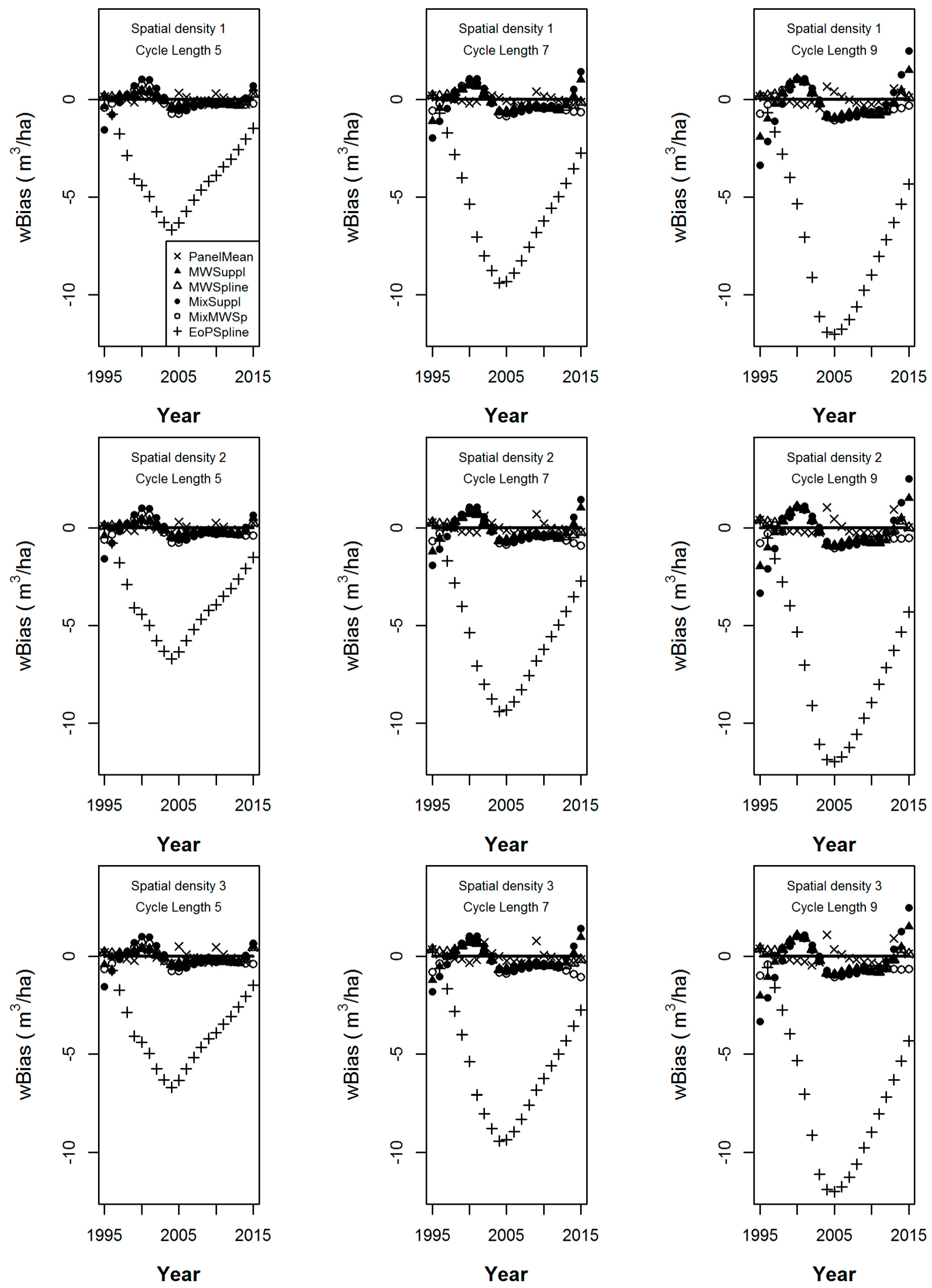
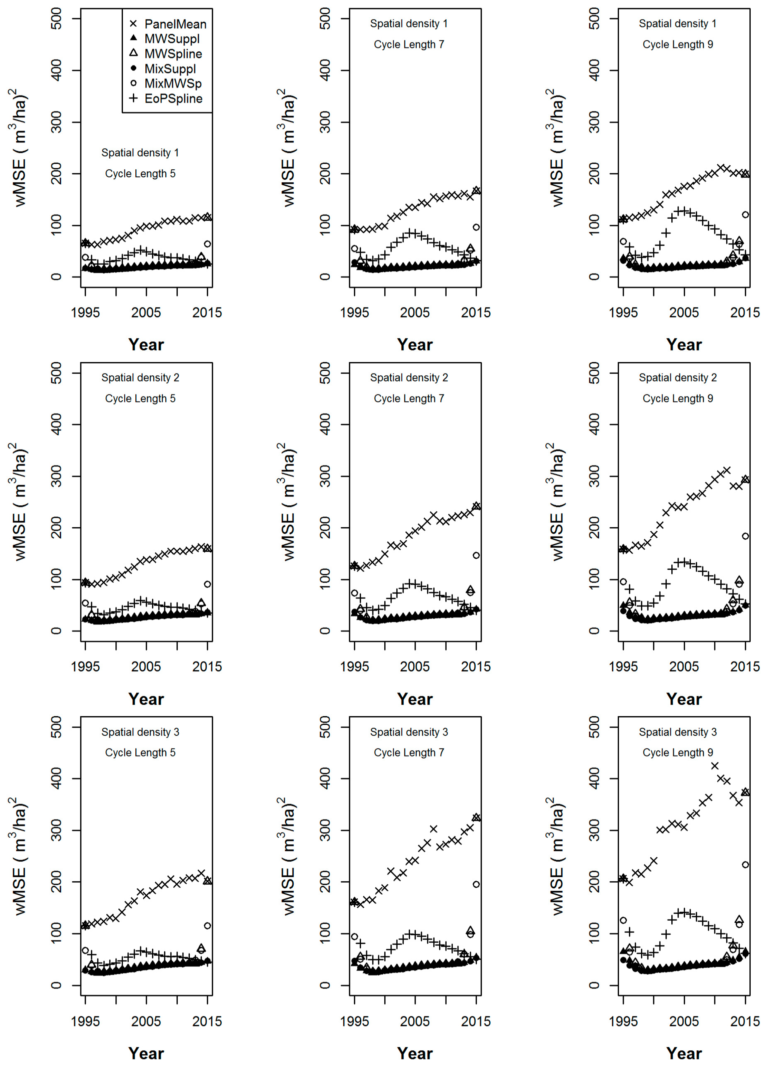
The wBias statistics calculated over the 152 populations of the estimators for cycle lengths of 5, 7 and 9 years from the simulation under sampling intensities 1 through 3 are given in Figure 3, while the corresponding wMSE statistics are given in Figure 4. In the nine graphs of each figure, increasing cycle length is shown from left to right, while decreasing sample intensity is shown from top to bottom.

We can make several observations that are common to the nine graphs in Figure 3. First, we note that the panel mean is the only design-unbiased estimator. All of the other estimators show bias in the annual estimates, the magnitude of which depends on how well their underlying models fit the individual population trajectories. Often, that bias is not much greater than the empirical bias of the panel mean. EOPSpline is almost always the most biased except for estimates made for the years 1995 and 1996. Note that in 1995, EOPSpline is equal to the panel mean, given that data for only 1 year are available. The supplemented estimators (MWSuppl and MixSuppl) show more bias in Figure 3, but lower wMSE (in Figure 4) in the extraneous years than their splined estimator (MWSpline and MixMWsp) counterparts. In Figure 3, as cycle length increases (from the left to the right graphs), the wBias of all estimators except the panel mean increases, with that of the EOPSpline being the most exaggerated.

In Figure 4, in the extraneous years, as cycle length increases, the wMSE of all estimators correspondingly increases. We note no significant change in the wMSE ranking of the estimators for specific years or between years in the non-extraneous years for each cycle length. We do observe differences in the wMSE rankings between the three temporal groupings of (1) the lower extraneous years, (2) the non-extraneous years and (3) the upper extraneous years, for each cycle length. Recall that the number of extraneous (or extreme years) increases as cycle length increases, the effects of which can be seen from left to right in Figure 4.

As sample density decreases from top to bottom in Figure 3 we note minor changes in wBias magnitudes, but no change in wBias ranking of the estimators for each year. Also, for the corresponding graphs in Figure 4, there are proportional changes in wMSE magnitudes but no change in wMSE ranking of the estimators for each year.

4. Discussion

It is not often acknowledged that for the class of sample designs being discussed here, model-based estimators are required to ensure that annual estimates can be made with low variance. Model-based estimators can be model-unbiased but they are not design unbiased. As mentioned above, the panel mean is the only design-unbiased estimator that we consider here. The results show that the panel mean has such a high variance that most of the time is has the highest wMSE for the annual estimates. The magnitude of bias in the model-based estimators does depend on how well their underlying models fit the population trend, with EOPSpline being the least responsive to changes in trend. The supplemented estimators (MWSuppl and MixSuppl) show more bias but lower mean squared error in the extraneous years than their splined estimator (MWSpline and MixMWsp) counterparts. As cycle length increases, the bias of all of the model-based estimators increases, with the greatest effect showing in EOPSpline. All of the model-based estimators, except for EOPSpline, work well in the non-extraneous years, although there are differences in the rankings based on mean squared error between the three groupings of estimation years, the lower extraneous years, the non-extraneous years and the upper extraneous years. The decrease in spatial intensity is shown to contribute to minor changes in the magnitudes of bias and mean squared error, but those changes are less drastic than those observed to result from an equivalent reduction in plot observations effected through the lengthening of the cycle.

While it is true that all national forest inventories attempt to provide estimates of many different variables, and we have used only one in our simulation, we believe that we can cautiously think of the results of this study in somewhat more general terms. That is, although the variable of interest here was cubic meters per hectare of wood through a 21-year period, the estimators themselves are indifferent to the exact variable of interest. The conclusions here should apply to all variables that have about the same relationship of spatial to temporal diversity or rate of change. This would be true for many, but certainly not all variables of interest. Variables that have about the same spatial diversity but a faster rate of change through time would be more affected by a lengthening of the cycle and those with a slower rate of change through time would be less affected by a lengthening of the cycle, than what we observed in these simulations. All of these estimators are affected by how any particular variable changes over the landscape relative to how it changes through time.

In this study, we took the values of the variable of interest (cubic meters per hectare) at face value, rather than treating those values as derivatives of observed values, and then explicitly incorporating the additional model error in the sampling simulations. We do not know if the error associated with the application of volume equations would suggest that larger errors in the sampling simulations should be considered. One reason is that there are many tree species for which no volume equations have been developed. Typically, in those cases, a volume equation developed for a different, but presumably similar, species is used. Additionally, populations of specific species could be changing enough through time that older volume equations have greater error than they once had. These unknowns can only be addressed through future research. Some of this research is currently being conducted, as the improvement of volume equations for many, but not all, species is an area of active research in the USA and worldwide.

5. Conclusions

This study did show some differences in the abilities of the estimation systems and their variants to provide estimates in the extreme years. Naturally, the distinctions between these estimators would become less important for variables that show little change through time. The effect of lengthening the cycle relative to reducing the spatial intensity of the plots would also become less drastic in that case. If a variable happened to have a higher spatial diversity and/or lower temporal diversity than our variable of interest, then our conclusions might have been quite different.