Article

Species Diversity, Stand Structure, and Species Distribution across a Precipitation Gradient in Tropical Forests in Myanmar

1
Department of Environmental Horticulture, University of Seoul, Seoul 02504, Korea
2
Department of Biological and Environmental Science, Dongguk University, Gyeonggi 10326, Korea
*
Author to whom correspondence should be addressed.
Forests 2017, 8(8), 282; https://doi.org/10.3390/f8080282
Submission received: 16 June 2017 / Revised: 2 August 2017 / Accepted: 3 August 2017 / Published: 4 August 2017

Abstract

:
An understanding of how species diversity, structural pattern, and species distribution vary across different environmental regions is crucially important for tropical ecology. In this study, we explored how these ecological parameters vary across various rainfall regions in the tropics with annual rainfall levels ranging from 843 to 2035 mm. Diversity, similarity, structure, and forest classification, and their correspondence with rainfall regions were tested. We found that species diversity, site class, and structural complexity increased with rainfall, with differences of 1000 mm having significant effects on diversity. The structure and heterogeneity of forests were higher in the high rainfall regions than the low rainfall regions. The forest structure was significantly correlated with rainfall, and the structure differed substantially where annual rainfall differed among sites by approximately 200 or 400 mm. Forests could be classified into two types according to whether they had high annual rainfall (1411–2035 mm) or low annual rainfall (843–1029 mm). In addition, the dominance of species changed noticeably from high- to low-rainfall regions, with Tectona hamiltoniana and Terminalia oliveri only being abundant in the low rainfall region. Species diversity and richness were significantly correlated with rainfall and average temperature. These findings will provide invaluable information for forest management and ecological phytogeography.

1. Introduction

Species diversity and stand structure are essential for forest biodiversity because trees provide the basic needs and habitat for other species [1,2,3]. It has been broadly accepted that species distribution and structure and their response to environmental factors are core concepts for ecological study [4,5,6]. In addition, an understanding of the diversity and stand structure of forests is critical for climate change regulation because their manipulation can allow creation of forests that absorb more carbon dioxide [7,8]. Therefore, it is important that forests are constantly monitored to determine whether diversity is being maintained. However, although much attention has been given to biodiversity conservation and how biodiversity varies between different forest conditions [1,9], we still only have a limited understanding of how forest diversity and structure vary between different rainfall regions because such forests always occur in different regions with different climates [9,10,11,12].
Recent studies have examined the relationship between species diversity and climatic effects [13,14,15,16]. For example, models that describe the broad-scale relationships between climate and woody plant richness have been developed by Field et al. [13] and, for angiosperms, by Francis and Currie [14]. Field et al. [13] demonstrated that species richness increased with temperature up to a maximum, beyond which water deficiency then tended to reduce richness [13,17], while Goldie et al. [18] found that water availability played a key role in the evolutionary processes of woody plants in arid regions, with persistent drought reducing the rate of these processes. Sixty-three and sixty-eight percent of global variability in angiosperm and woody plant family richness, respectively, were explained by rainfall [13,14,15].
Similarly, it has been found that species richness increased with precipitation until it reached 4000 mm in a neotropical region [16]. Moreover, rainfall has been shown to have a positive effect on the diameter, basal area [7,19], and carbon storage [20] of forests. In addition, Wang et al. [21] observed that the number of species and the rate of species turnover increased with temperature within a range of −12 °C to 20 °C. However, the relationship between temperature and species richness has been shown to be negative under limited water availability [17].
Forest structure may also show marked variation among continents [16]. For example, a negative relationship has been found between latitude and the annual net primary productivity of forests [22]. Tropical forests are rich in biodiversity and contain a significant proportion of global biodiversity [23,24], and they vary geographically depending on evolutionary history and climate [7,23,24]. Thus, knowledge of how the diversity, distribution, and structure of tropical forests varies between rainfall regions is critical for tropical ecology. Furthermore, species–environmental relationships can be used as indicators of environmental conditions, and the diversity and patterns of forests can be used to elucidate ecological phytogeography [25,26]. However, despite the importance of this information, few detailed data have been obtained for tropical forests [26]. Thus, the floristic diversity and distribution patterns in tropical forests in Southeast Asian regions, especially in Myanmar, remain poorly understood, even though several studies have been conducted under different management techniques [27,28,29] or in individual regions [29,30].
Myanmar has some of the richest biodiversity in the Indo-Pacific region and one of the highest forest proportions in the Southeast Asian region, with forests covering 44.2% of the total land area [31]. In addition, there is a variety of climatic conditions throughout the country. Therefore, in this study, we examined the species distribution, stand structure and diversity of forests in different rainfall regions of Myanmar. The main goal of this research was to improve our understanding of ecological phytogeography in this region. The results of this study may provide insight into forest management and ecological study that would be applicable to other tropical countries. To achieve the main goal of this study, we addressed two main questions: (1) do forest diversity and stand structure vary across different rainfall regions in the tropics; and (2) If so, how do the species distribution and stand structure of forests vary with different rainfall regions?

2. Materials and Methods
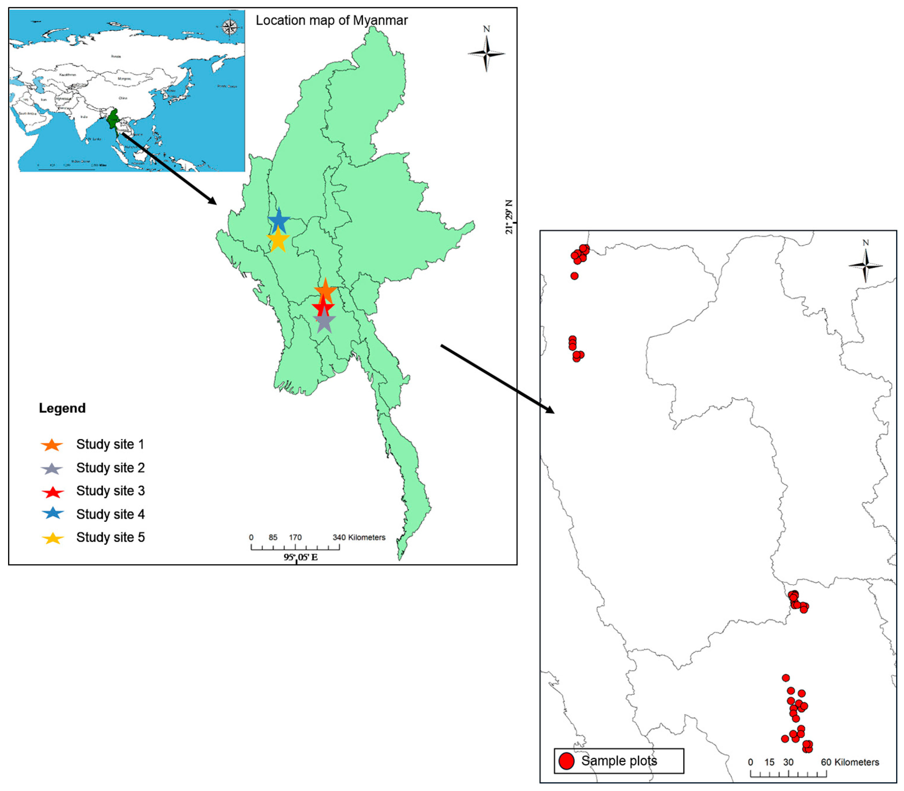
2.1. Study Area

The studies were conducted in five study areas with different mean annual rainfall levels, ranging from 843 to 2035 mm (Figure 1): site 1 in “Yaedashae” (19°15′–19°23′ N, 95°51′–95°58′ E); site 2 in “Gyobingauk” (18°15′–18°24′ N, 95°49′–95°59′ E); site 3 in “Nattalin” (18°28′–18°46′ N, 95°49′–95°57′ E); site 4 in “Pauk” (21°38′–21°49′ N, 94°19′–94°24′ E); and site 5 in “Seikphyu” (21°02′–21°11′ N, 94°18′–94°22′ E). All of the study sites contained tropical deciduous forests that were protected as reserve forests, and diverse species and a variety of structures were distributed throughout the region. These forests provide habitats for endangered tree species such as Dipterocarpus grandifloras (critically endangered; CR), Dalbergia oliveri (endangered; EN), and Dalbergia cultrata (nearly threatened; NT) [32,33]. The forests are also home to several protected animals, such as elephant (Elephas maximus, EN), deer (Rucervus eldii, EN), gibbon (Hylobates lar, EN), green peafowl (Pavo muticus, EN), and clouded leopard (Neofelis nebulosi, vulnerable [VU]) [32,34]. The forests include economically important species and are managed sustainably by the Myanmar selection system. Illegal cutting was found in some places, which we avoided collecting data from.
This region has a tropical savanna climate. During 1982–2014, the mean annual rainfall levels at study sites 1, 2, 3, 4 and 5 were 2035 mm, 1600 mm, 1411 mm, 1029 mm and 843 mm, respectively (Department of Meteorology and Hydrology of Myanmar, unpubl. data), while the average maximum rainfall was 476 mm (August), 323 mm (June), 290 mm (June), 200 mm (September), and 191 mm (September), respectively. The rainy season is from May to October. The mean annual temperatures at study sites 1, 2, 3, 4 and 5 were 27 °C (maximum 38.1 °C), 27 °C (maximum 38.7 °C), 27.2 °C (maximum 38.8 °C), 24.1 °C (maximum 34.6 °C), and 25.7 °C (maximum 36.2 °C), respectively, indicating that there was little variation in temperature among the study sites. The warmest month of the year was April (May at site 5) and the coldest month of the year was January. In this study, we used the term “high-rainfall region” to describe site 1 and “low-rainfall region” to describe site 5, with sites 2–4 falling between these extremes.

2.2. Sampling Procedures and Data Analysis

Sampling plots (50 × 50 m; 2500 m2) were established at each study site using the stratified random sampling method. A preliminary site investigation was carried out in each of the selected areas before establishing the sample plots, following which the forests were stratified according to the appearance of tree density, coverage and the presence of minor disturbance. The plots were then established randomly in each stratum so that they encompassed all levels of these variables within the selected forests. To ensure that the sample size was sufficiently large to represent the entire population, we developed species-area curves to determine the minimum representative area for each population (Figure 2). This is a widely accepted method whereby the minimum sample size is considered to be the point where the curve becomes flattened [30,35,36]. Based on these curves, we sampled 2.75 ha (11 plots) at site 1, 2.25 ha (9 plots) at site 2, 2.5 ha (10 plots) at site 3, 2.5 ha (10 plots) at site 4 and 1.5 ha (6 plots) at site 5.
We measured the diameter at breast height (dbh) and height of all trees with a diameter >5 cm in each of the sample plots, and used this to calculate the quadratic mean diameter of forests and to group the trees into diameter classes at 10-cm intervals. The height layers were also divided into three groups: upper layer (>2/3 of top height), middle layer (<2/3 to >1/3 of top height), and lower layer (<1/3 of top height) [37,38]. To determine the heterogeneity of the forest, we constructed frequency diagrams based on the occurrence of species in each frequency class (frequency class I = 1–20%, II = 20–40%, III = 40–60%, IV = 60–80% and V = 80–100%) [30,38]. The frequency of a given species was calculated as its percentage occurrence across all of the sample plots in a particular area. We also calculated the importance value index (IVI) for each species to determine the dominant species in each forest [37,38]. To characterize the forests, we determined the relative density, basal area, relative frequency and relative coverage of each forest type per hectare. Identification of species was performed using “Forest flora of British Burma” [39] and completed at the Plant Taxonomy and Seed Storage Division, Forest Research Institute, Myanmar. We estimated species richness using Jackknife species richness [40].
We used one-way analysis of variance (ANOVA) followed by Duncan’s multiple range test (DMRT) to determine differences in diameter, height, basal area, and density of trees among study sites and an independent-samples t-test to examine differences in species composition between lower and higher frequency classes. Cluster analysis was applied to determine the variation between frequency classes at all study sites.
The diversity of forests was assessed using two common species diversity indices: the Shannon index [41] and the Simpson index [42]. The Shannon diversity index favors rare species, while the Simpson diversity index favors more abundant species [37,43,44]. We also calculated the Shannon evenness to define how close in numbers each species was in an environment [41]. One-way ANOVA followed by DMRT was then used to determine whether there were any significant differences in these indices among sites.
The similarity among different forest types was evaluated using both presence/absence and abundance measures. Sorenson’s similarity index [38], Lamprecht modification’s index [38] and Sorenson’s quantitative index [45] were used in this study. The forest type was classified using cluster analysis based on the ecological distance (Bray measure) among forests in the R program.
Variation in the species distribution and abundance across the study forests was illustrated by correspondence analysis (CA) using both species and site scores. The statistical relationship between climatic variables (such as mean annual rainfall, maximum rainfall, mean annual temperature, and the maximum–minimum difference between the warmest and coldest month [T dif]) and the attributes of diversity, richness, diameter and height of forests were evaluated by Pearson’s correlation coefficients.
All statistical analyses in this study were performed in the R program and SPSS statistical software.

3. Results

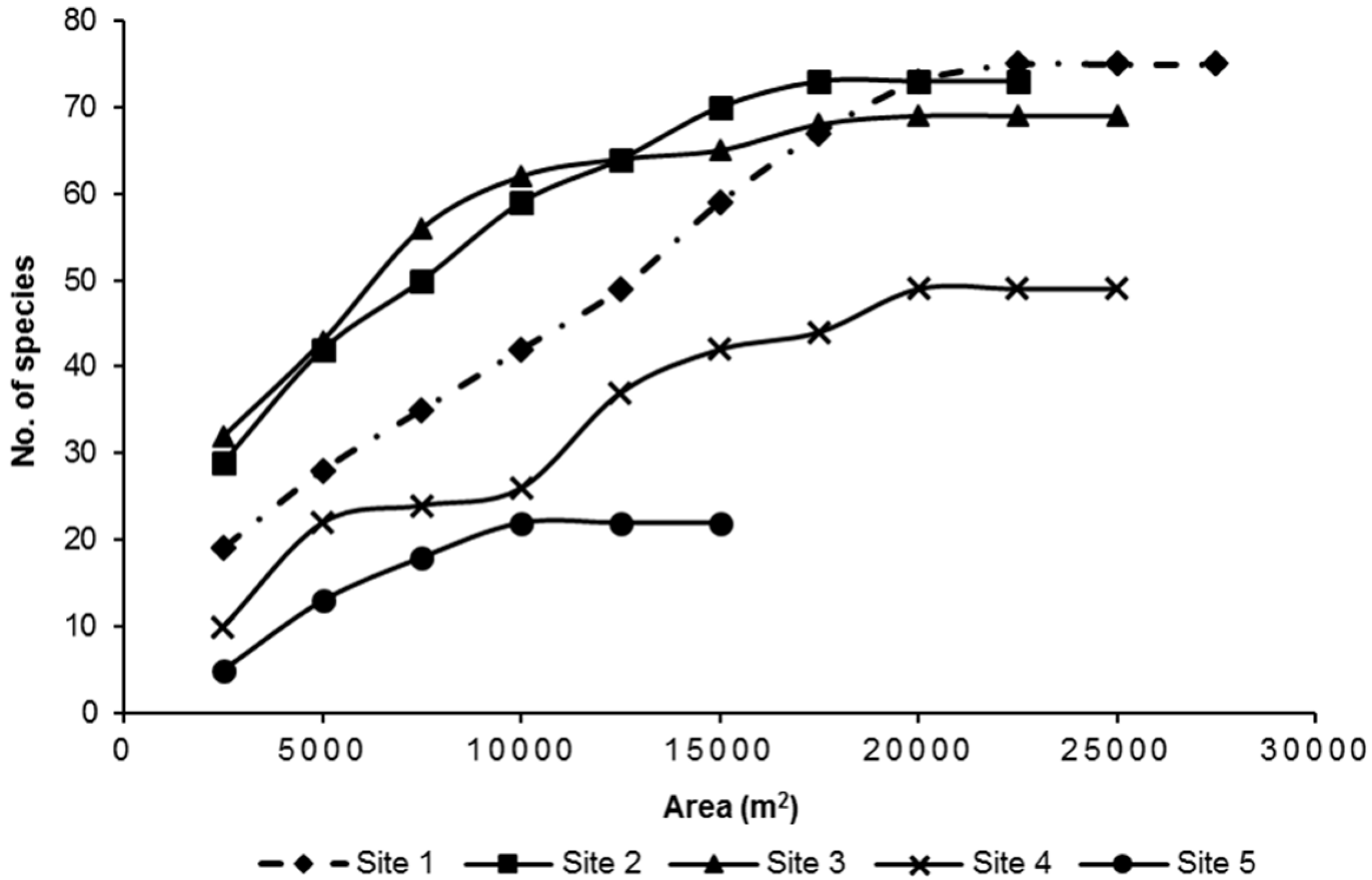
3.1. Species Diversity

The Jackknife estimates for species richness at sites 1, 2, 3, 4, and 5 were 75.83, 73.79, 69.73, 49.81, and 23.00, respectively. A total of 75 species (31 families), 73 species (29 families), and 69 species (25 families) were found at sites 1, 2 and 3, respectively, while 49 species (24 families) and 22 species (12 families) were found at sites 4 and 5. Thus, species richness was higher at site 1 than at the other sites with lower annual rainfall.
Diversity of forests was determined using the Shannon and Simpson diversity indices (Table 1). The Shannon diversity index, evenness and Simpson diversity index tended to increase with increasing rainfall and significantly differed among forests (ANOVA, p < 0.05), with sites 1–3 exhibiting significantly higher diversity than sites 4 and 5 (DMRT, p < 0.05) (Table 1).

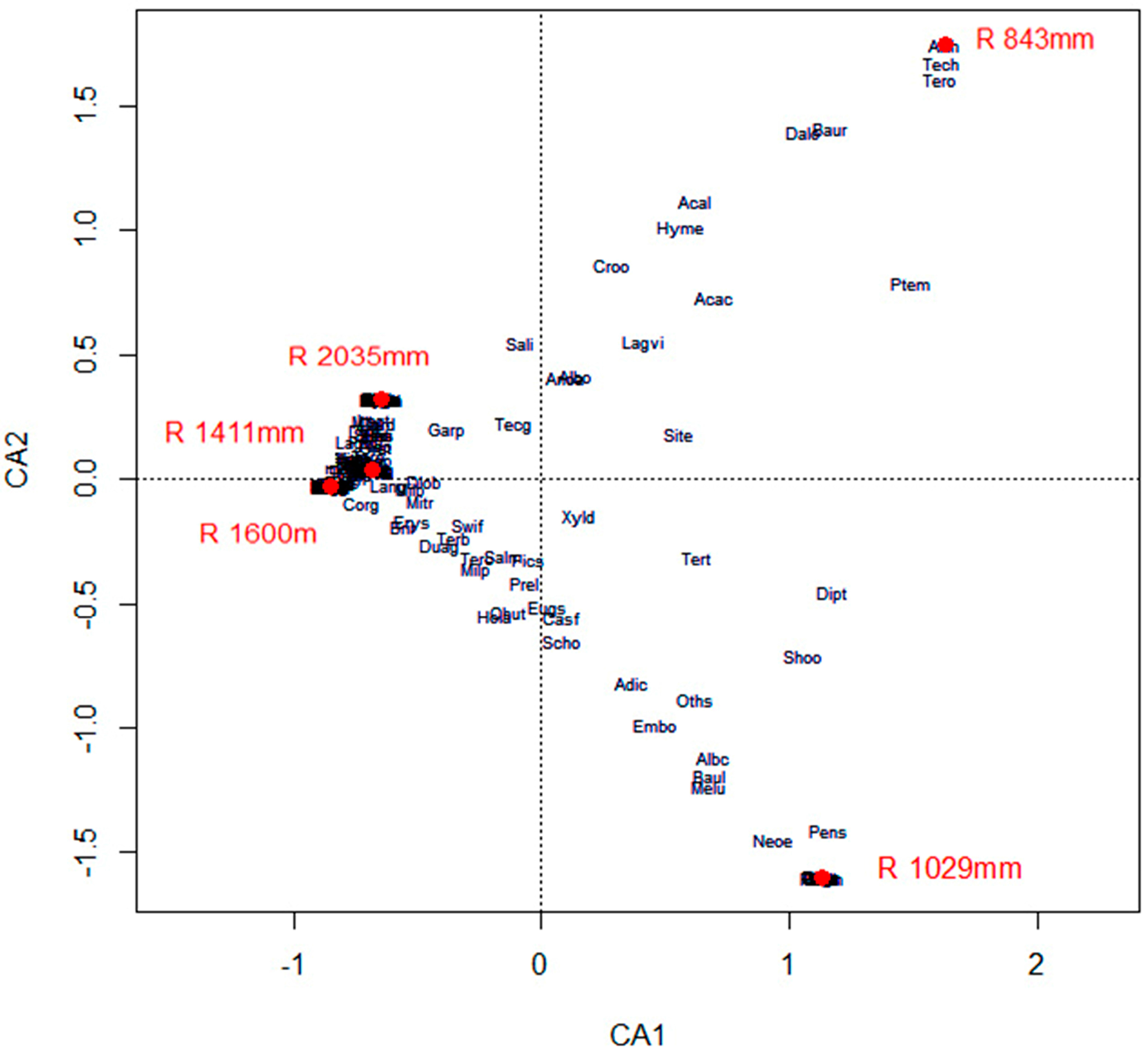
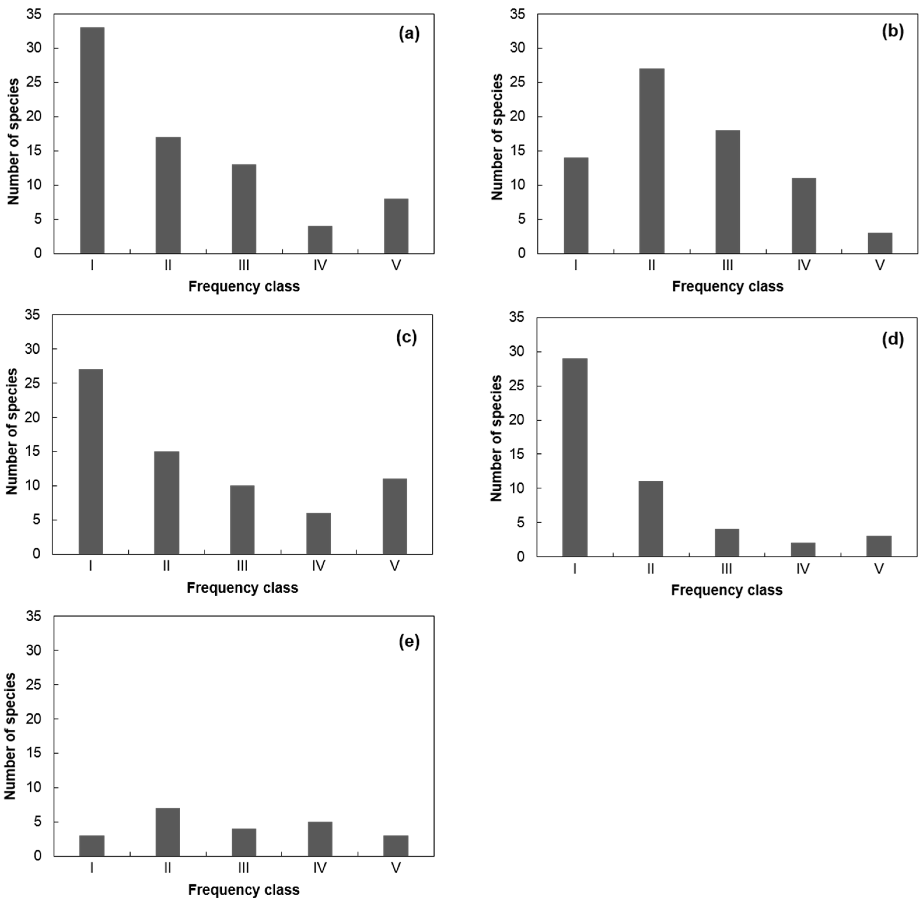
3.2. Species Composition and Distribution

The basal area and density of species varied both within and among forests. For example, at site 1, the basal area of Quercus brandisiana was 0.004 m2 ha−1, while that of the dominant species, Xylia dolabriformis, was 6.13 m2 ha−1. By contrast, the basal area of X. dolabriformis was only 2.78 m2 ha−1 at site 2, despite also being one of the dominant species at this site.
Xylia dolabriformis, Tectona grandis, Protium serrata, Mitragyna rotundifolia, and Lagerstroemia tomentosa were the five most dominant species in terms of IVI values at site 1, where the annual rainfall was 2035 mm. However, where annual rainfall differed among sites by approximately 400 mm or more, the dominant species and their proportions also differed substantially. For example, we found that X. dolabriformis, Cordia grandis, M. rotundifolia, Dalbergia cultrata, and Lannea grandis were the dominant species at site 2, where the annual rainfall was 1600 mm, while T. grandis, which was one of the five most dominant species at site 1, was the ninth-most dominant species here. Similarly, the species dominance at site 3 was different from site 1 and site 2, with X. dolabriformis, Terminalia tomentosa, M. rotundifolia, Tectona grandis, and P. serrata being the five most dominant species, among which Terminalia tomentosa was in the 24th and 26th position of the species dominance at site 1 and site 2, respectively.
At site 4, where the annual rainfall was approximately 1000 mm lower than that at site 1, X. dolabriformis, Pentacme siamensis, Terminalia tomentosa, Shorea oblongifolia, and Dipterocarpus tuberculatus were the most dominant species, among which P. siamensis did not occur at sites 1 to 3. Finally, at site 5, where the annual rainfall was approximately 1200 mm lower than that at site 1, the most dominant species changed completely. The most dominant species were T. hamiltoniana, X. dolabriformis, Terminalia oliveri, Terminalia tomentosa, and Anogeissus acuminata (see at site 5), while P. serrata, which was the second-most dominant species at site 1, did not occur. The IVI, relative density, relative frequency, and relative coverage of 20 dominant species in the forests at the five study sites are shown in Tables S1–S5. The family composition and frequency also varied among the five study sites (Table 2), with the most frequently occurring families at sites 1, 2, 3, 4, and 5 being Fabaceae (12.2%), Fabaceae (9.7%), Anacardiaceae (8.7%), Combretaceae (10.4%), Mimosaceae (19%), respectively.
Frequency diagrams were used to illustrate the heterogeneity of the forests—a forest stand is considered heterogeneous when most of the species are found in the lower frequency classes. Reciprocally, when most of the species occur in higher frequency classes, then that stand can be considered homogeneous. In this study, frequency diagrams showed the complete representations of species in all of the frequency classes at all of the study sites (Figure 3), showing the number of species varied among frequency classes at all of the study sites (cluster analysis). Moreover, the significantly higher numbers of species in the lower frequency classes than the higher frequency classes (t = 4.255, p = 0.001) demonstrated that all of the forests were heterogeneous. However, forests at sites 1–4 had greater heterogeneity than that at site 5, as indicated by the higher ratio of lower classes to higher classes (>50% of species fell in lower frequency classes and a maximum of 23% fell in higher frequency classes at sites 1–4, compared with 44% and 35%, respectively, at site 5).

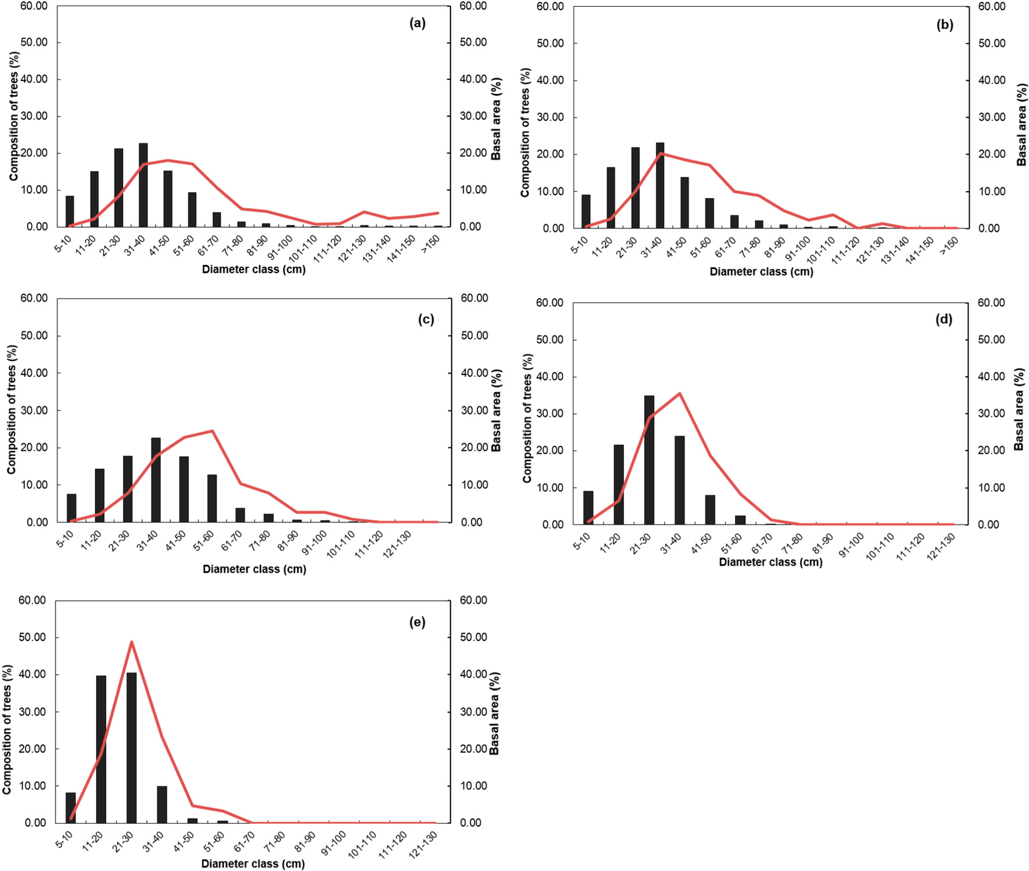
3.3. Stand Structure

Stand structure relates to the distribution of tree growth or species within a forest stand and can thus reflect the interaction between vegetative growth and environmental conditions [46,47]. In this study, we focused on both horizontal and vertical stand structures.
Basal areas and densities of the forests varied among the sites. The basal areas were 43.41 ± 2.2, 41.11 ± 2.18, 39.66 ± 2.20, 20.23 ± 2.98, and 8.92 ± 0.82 m2 ha−1 at sites 1–5, respectively, while the densities were 336 ± 36.55, 368 ± 30.03, 325 ± 24.30, 322 ± 33.85, and 229 ± 23.11 trees ha−1, respectively. Site 5 had a significantly lower basal area and density than the other sites (DMRT, p < 0.05) (Table S6).
The quadratic mean diameters of the forests were 40.58 cm, 37.69 cm, 39.40 cm, 28.30 cm, and 22.28 cm for sites 1–5, respectively. The distribution of diameters had a positive skewness in all of the forest stands. However, the diameter size classes decreased in the order of sites 1 to 5, with diameter size classes >100-cm dbh comprising 6.41 m2 ha−1 (14.76%) of the total basal area at site 1, 2.06 m2 ha−1 (5.02%) at site 2, and 0.33 m2 ha−1 (0.82%) at site 3, and the largest diameter size class being 61–70 cm at site 4, which covered 0.26 m2 ha−1 (1.27%) of the total basal area, and 51–60 cm at site 5, which covered 0.58 m2 ha−1 (3.33%) of the total basal area (Figure 4). The composition of trees was highest in the 21–40-cm dbh class at sites 1 and 2, the 31–40-cm dbh class at site 3, the 21–30-cm dbh class at site 4, and the 11–30-cm dbh class at site 5.
As with horizontal structure, the vertical structure in terms of the height, diameter, basal area, and tree density through the upper, middle and lower layers of forests exhibited a decreasing trend from site 1 to site 5 (Table 3), with average tree heights of the upper, middle, and lower layers ranging from 49.45 m, 23.35 m, and 12.6 m, respectively, at site 1 to 14.17 m, 8.96 m, and 5.09 m, respectively, at site 5, which represented 28.65%, 38.37%, and 40.40% of the site 1 heights. In addition, the top height of the forest was greatest at site 1 (55.37 m) and the lowest at site 5 (18.15 m).
All of the forests had the lowest density in the upper layer (2.06%, 6.63%, 15.50%, 8.33% and 11.66% of total coverage at sites 1–5, respectively) and the highest basal area in the middle layer (54.24%, 62.42%, 55.27%, 71.41% and 64.08% of total basal area at sites 1–5, respectively). However, the basal area of the lower stratum at site 1 where the highest rainfall occurred, represented a significantly higher percentage of the total basal area (27.02%) than that of the other lower rainfall regions ( DMRT, p < 0.05) (Table 3).

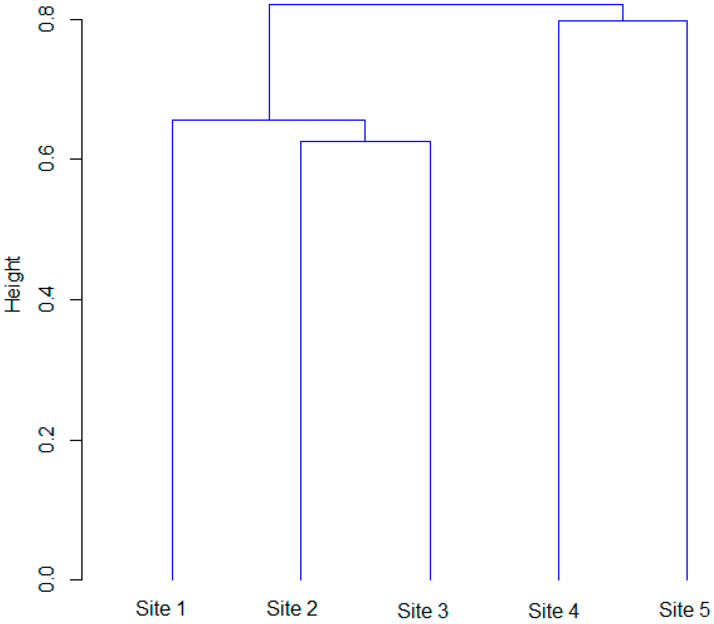
3.4. Similarity of Forests

Sorenson’s index, the Lamprecht modification index, and Sorenson’s quantitative index showed that the study forests differed according to the presence/absence and abundance of species, with sites 1, 2, and 3 having >55% similarity, and site 5 showing the least similarity to sites 1–4 (Table 4). However, the percentage similarity between sites 5 and 4 was higher than that between site 5 and sites 1–3.
The forests could be classified into two groups based on ecological distance (Figure 5). A dendrogram showed that the ecological distances were closer between sites 1–3 and between sites 4 and 5, indicating that the forests with an annual rainfall of 1411–2035 mm could be considered as one group while those with an annual rainfall of 843–1029 mm could be considered a separate group.

3.5. Effects of Climate on Diversity, Distribution, Diameter and Height of Forest

The diversity, richness, diameter, and height of forests were affected by environmental factors such as annual rainfall, annual temperature, and T dif. Species diversity and richness were significantly correlated with annual rainfall, maximum rainfall and average temperature. There were also significant positive correlations between forest diameter and height and rainfall parameters such as mean annual rainfall and maximum rainfall (p < 0.01; Table 5). Rainfall had a stronger effect on forest structure than temperature within a rainfall range of 843–2035 mm and a temperature range of 24.1 °C–27.2 °C, although both rainfall and temperature were important for forest structure. T dif did not vary greatly among the five sites (22.2 °C–23.3 °C) and so did not have a significant effect on forest structure.
CA indicated that there was a clear correlation between both species distribution and abundance and annual rainfall (Figure 6). The first and second CA axes explained 65.28% of the total fitted variation. The weighted average scores of species under different rainfall levels varied to a great extent in terms of abundance and distribution, spreading into different quarters of the ordination graph. Sites for which the rainfall parameter is located close to the species on the graph are expected to have a high abundance of that species. For example, Pentacme siamensis (Pens) was abundant in the region where rainfall was 1029 mm (Figure 6), whereas the region with 2035 mm rainfall was not an appropriate habitat for that species. A small vector angle between species indicated a strongly positive association, and a 180-degree vector angle between species indicated a negative correlation.

4. Discussion

It has previously been shown that stand structure can be predicted by climatic factors at both the local and regional levels [8,16,48,49], while species diversity is significantly influenced by the structure and composition of forests [2]. Furthermore, the diversity and composition of forests may vary with different forest types and stages [43,50,51,52,53]. The results of our study are in agreement with these findings, as the diversity, distribution, and composition of forests varied between regions with different annual rainfall levels but similar annual temperatures variations. Thus, it appears that rainfall has a strong effect on the diversity, richness and evenness of forests, with each of these tending to decrease with a decrease in rainfall (Table 1). The results of this study were consistent with the findings of Osland et al. [54] and Staver et al. [55]. In addition, significant differences in species diversity and richness were observed among forests with an annual rainfall of 843–1029 mm and those with an annual rainfall of 1411–2035 mm (Table 1).
This study was conducted in areas where the annual rainfall ranged from 843 mm to 2035 mm. The species diversities at each of the study sites was higher than previously observed in dry Diospyros forests (1.71) [30] and Acacia forest (0.43) [30] of the central dry zone in Myanmar, but similar to those found by Oo [37] in similar forests types in Myanmar.
Species belonging to the families Fabaceae, Lythraceae, Mimosaceae and Combretaceae primarily occurred at site 1 (high rainfall), but only one species of the Lythraceae family was found at site 5 (low rainfall). By contrast, the families Mimosaceae, Combretaceae, Verbenaceae and Diptocarpaceae were primarily found at site 5 (low rainfall), while only one species of Lythraceae and a low abundance of Fabaceae were found here. Some families were absent from low-rainfall areas. For example, Sterculiaceae and Anacardiceae were present at site 1 (annual rainfall = 2035 mm) but absent from site 5 (annual rainfall = 843 mm). Furthermore, although Anacardiceae was observed at site 4 (annual rainfall = 1029 mm), Sterculiaceae was not. Therefore, Anacardiceae could be found in regions with annual rainfall of 1029–2035 mm, while Sterculiaceae was present in regions with annual rainfall of 1411–2035 mm.
Species distribution was strongly correlated with climatic variation and was more affected by annual rainfall than temperature [4]. Relative abundance has been shown to vary with geographic distribution and vegetation zones [3]. Based on the results of our study, Tectona hamiltoniana represented the forests in the region with approximately 800 mm of annual rainfall, along with the associated species X. dolabriformis and Terminalia oliveri (Table S5), with a relative coverage of 45.44% of the total. By contrast, an equal association of Pentacme siamensis, X. dolabriformis and Terminalia tomentosa represented the forest in the region with approximately 1000 mm of annual rainfall (relative coverage = 42.54%). In the regions with approximately 1400 mm of annual rainfall, the predominant species were X. dolabriformis, Terminalia tomentosa, Mitragyna rotundifolia, Tectona grandis, Protium serrata, and Salmalia insignis (relative coverage = 34.78%), whereas the region with 1600 mm of annual rainfall was represented by several species including X. dolabriformis, Cordia grandis, M. rotundifolia and Tectona grandis (relative coverage of the 10 dominant species = 38.37%). Finally, the region where the annual rainfall was approximately 2000 mm was dominated by X. dolabriformis, Tectona grandis, Protium serrata, M. rotundifolia and Lagerstroemia tomentosa (relative coverage = 39.39%).
High-rainfall regions (1411–2035 mm) did not contain Tectona hamiltoniana and Terminalia oliveri and those species also rarely occurred in regions with 1029 mm of annual rainfall (relative coverage = 0.57%). However, these species were abundant in regions with 843 mm of annual rainfall (relative coverage = 34.56%).
Both species richness and forest structure were significantly correlated with rainfall, and species richness was also significantly correlated with average temperature (Table 5). We found that the number of species was higher at high rainfall regions than the low rainfall regions, with site 1, which had the highest rainfall among the five sites, also having the greatest species richness (1.5- and 3.4-fold higher than at sites 4 and 5, respectively, where the annual rainfall was approximately 1000 mm and 1200 mm lower) (Table 1).
The number of species that were found at site 1 (75 species, 31 families) was similar to the previous findings for subtropical evergreen forests in Japan (77 species, 33 families) [56] and tropical forests in Central Africa (73 species, 25 families) [57]. However, the number of species at other sites (sites 1–4) were lower than observed in these forests. A comparison of the species richness between the forests in Myanmar shows that the richness observed in this study was approximately 2.5–5 times lower than that in national parks containing tropical evergreen forests [37] and 2–6 times higher than that in dry Diospyros forests of the dry zone [30].
These findings have important implications for phytogeography and ecology, giving insight into the effects of annual rainfall on the species distribution, diversity, richness, structure, and coverage in tropical regions.
The critically endangered species Dipterocarpus grandifloras only occurred at site 1, where it had a relative coverage of 0.56%. The endangered species Dalbergia oliveri occurred at sites 1 and 5, with a relative coverage of 0.05% and 1.09%, respectively, while the nearly threatened species Dalbergia cultrata covered at sites 1–3, with a relative coverage of 0.18%, 4.52% and 3.96%, respectively. These species need to be protected and managed for their survival in these tropical forests.

5. Conclusions

In this study, we found that the species diversity and structure of tropical forests in Myanmar varied with rainfall region. This finding supports the previously proposed hypothesis that species diversity is correlated with climate factors. In these forests, the basal area, size class, and stand structure consistently decreased from high- to low-rainfall regions, as did species richness. The species dominance also differed from high- to low-rainfall regions. Furthermore, a difference in annual rainfall of approximately 600 mm among sites did not significantly affect species diversity in this savanna climate (annual rainfall = 843–2035 mm), but a difference of approximately 1000 mm had significant effects. Based on our findings, species richness was significantly correlated with rainfall and average temperature, while forest structure was significantly correlated with rainfall. Given that rainfall and temperature are the key variables for productivity, our finding is consistent with studies showing a positive relationship between productivity and species richness in forests. Species distribution varied markedly between high- and low-rainfall regions; for example, Xylia dolabriformis and Tectona grandis could spread from high- to low-rainfall regions, but exhibited reduced growth in the latter, whereas Tectona hamiltoniana and Terminalia oliveri were abundant only in the low rainfall region. The results from this study will help to further our understanding and development of ecological phytogeography and management techniques in tropical regions.

Supplementary Materials

The following are available online at www.mdpi.com/1999-4907/8/8/282/s1, Table S1: Important value index, relative density, relative frequency and relative coverage of 20 dominant species of forests at study site 1, Table S2: Important value index, relative density, relative frequency and relative coverage of 20 dominant species of forests at study site 2, Table S3: Important value index, relative density, relative frequency and relative coverage of 20 dominant species of forests at study site 3, Table S4: Important value index, relative density, relative frequency and relative coverage of 20 dominant species of forests at study site 4, Table S5: Important value index, relative density, relative frequency and relative coverage of 20 dominant species of forests at study site 5, Table S6: Tree density and basal area of five study sites, Table S7: Species name and their abbreviations of five study sites.

Acknowledgments

This study was conducted with the financial support of ‘R&D Program for Forest Science & Technology (2012021E10-1718-AA01)’ provided by the Korea Forest Service (Korea Forestry Promotion Institute). We are grateful to everyone who helped with the field survey. We would like to thank two anonymous reviewers for their constructive comments.

Author Contributions

Inkyin Khaine, Su Young Woo and Hoduck Kang conceived and designed the experiments; Inkyin Khaine, MyeongJa Kwak, Sun Mi Je, Hana You, Taeyoon Lee, Jihwi Jang and Hyun Kyung Lee performed the experiments; Inkyin Khaine, Euddeum Lee, Li Yang, Haenaem Kim, JoungKyu Lee and Jieun Kim analyzed the data; Su Young Woo and Hoduck Kang contributed analysis tools; Inkyin Khaine and Su Young Woo wrote the paper.

Conflicts of Interest

The authors declare no conflict of interest.

References

  1. Cannon, C.H.; Peart, D.R.; Leighton, M. Tree species diversity in commercially logged Bornean rainforest. Science 1998, 281, 1366–1368. [Google Scholar] [CrossRef] [PubMed]
  2. Huang, W.; Pohjonen, V.; Johansson, S.; Nashanda, M.; Katigula, M.I.L.; Luukkanen, O. Species diversity, forest structure and species composition in Tanzania tropical forests. For. Ecol. Manag. 2003, 173, 11–24. [Google Scholar] [CrossRef]
  3. Reilly, M.J.; Spies, T.A. Regional variation in stand structure and development in forests of Oregon, Washington, and inland Northern California. Ecosphere 2015, 6, 1–27. [Google Scholar] [CrossRef]
  4. Amissah, L.; Mohren, G.M.J.; Bongers, F.; Hawthorne, W.D.; Poorter, L. Rainfall and temperature affect tree species distribution in Ghana. J. Trop. Ecol. 2014, 30, 435–446. [Google Scholar] [CrossRef]
  5. Condit, R.; Engelbrecht, B.M.J.; Pino, D.; Pérez, R.; Turner, B.L. Species distributions in response to individual soil nutrients and seasonal drought across a community of tropical trees. Proc. Natl. Acad. Sci. USA 2013, 110, 5064–5068. [Google Scholar] [CrossRef] [PubMed]
  6. Toledo, M.; Peña-Claros, M.; Bongers, F.; Alarcón, A.; Balcázar, J.; Chuviña, J.; Leaño, C.; Licona, J.C.; Poorter, L. Distribution patterns of tropical woody species in response to climatic and edaphic gradients. J. Ecol. 2012, 100, 253–263. [Google Scholar] [CrossRef]
  7. Khaine, I.; Woo, S.Y. An overview of interrelationship between climate change and forests. For. Sci. Technol. 2015, 11, 11–18. [Google Scholar] [CrossRef]
  8. Sevegnani, L.; Uhlmann, A.; Gasper, A.L.; de Meyeer, L.; Vibrans, A.C. Climate affects the structure of mixed rain forest in southern sector of Atlantic domain in Brazil. Acta Oecol. 2016, 77, 109–117. [Google Scholar] [CrossRef]
  9. Kalacska, M.; Sanchez-Azofeifa, G.A.; Calvo-Alvarado, J.C.; Quesada, M.; Rivard, B.; Janzen, D.H. Species compostion, similarity and diversity in three successional stages of a seasonally dry tropical forest. For. Ecol. Manag. 2004, 200, 227–247. [Google Scholar] [CrossRef]
  10. Feroz, S.M.; Kabir, M.E.; Hagihara, A. Species composition, diversity and stratification in subtropical evergreen broadleaf forests along a latitudinal thermal gradient in the Ryukyu Archipelago, Japan. Glob. Ecol. Conserv. 2015, 4, 63–72. [Google Scholar] [CrossRef]
  11. Johnson, C.; Chhin, S.; Zhang, J. Effects of climate on competitive dynamics in mixed conifer forests of the Sierra Nevada. For. Ecol. Manag. 2017, 394, 1–12. [Google Scholar] [CrossRef]
  12. Nlung-Kweta, P.; Leduc, A.; Bergeron, Y. Climate and disturbance regime effects on aspen (Populus tremuloides Michx.) stand structure and composition along an east-west transect in Canada’s boreal forest. Forestry 2017, 90, 70–81. [Google Scholar] [CrossRef]
  13. Field, R.; O’Brien, E.M.; Whittaker, R.T. Global models for predicting woody plant richness from climate: Development and evaluation. Ecology 2005, 86, 2263–2277. [Google Scholar] [CrossRef]
  14. Francis, A.P.; Currie, D.J. A globally consistent richness-climate relationship for angiosperms. Am. Nat. 2003, 161, 523–536. [Google Scholar] [CrossRef] [PubMed]
  15. O’Brien, E.M. Water-Energy dynamics, climate, and prediction of woody plant sciences richness: An interim general model. J. Biogeogr. 1998, 25, 379–398. [Google Scholar] [CrossRef]
  16. Gentry, A.H. Changes in plant community diversity and floristic composition on environmental and geographical gradients. Ann. Mo. Bot. Gard. 1988, 75, 1–34. [Google Scholar] [CrossRef]
  17. Gillman, L.N.; Wright, S.D. Species richness and evolutionary speed: The influence of temperature, water and area. J. Biogeogr. 2014, 41, 39–51. [Google Scholar] [CrossRef]
  18. Goldie, X.; Gillman, L.; Crisp, M.; Wright, S. Evolutionary speed limited by water in arid Australia. Proc. R. Soc. B 2010, 277, 2645–2653. [Google Scholar] [CrossRef] [PubMed]
  19. Toledo, M.; Poorter, L.; Pena-Claros, M.; Alarcon, A.; Balcazar, J.; Leano, C.; Licona, C.; Lianque, O.; Vroomans, V.; Zuidema, P.; et al. Climate is a stronger driver of tree and forest growth rates than soil and disturbance. J. Ecol. 2011, 99, 254–264. [Google Scholar] [CrossRef]
  20. Fischer, R.; Armstrong, A.; Shugart, H.H.; Huth, A. Simulating the impacts of reduced rainfall on carbon stocks and net ecosystem exchange in a tropical forest. Environ. Model. Softw. 2014, 52, 200–206. [Google Scholar] [CrossRef]
  21. Wang, Z.; Brown, J.H.; Tang, Z.; Fang, J. Temperature dependence, spatial scale, and tree species diversity in eastern Asia and North America. Proc. Natl. Acad. Sci. USA 2009, 106, 13388–13392. [Google Scholar] [CrossRef] [PubMed]
  22. Gillman, L.N.; Wright, S.D.; Cusens, J.; McBride, P.D.; Malhi, Y.; Whittaker, R.J. Latitude, productivity and species richness. Glob. Ecol. Biogeogr. 2015, 24, 107–117. [Google Scholar] [CrossRef]
  23. Sullivan, M.J.P.; Talbot, J.; Lewis, S.L.; Phillips, O.L.; Qie, L.; Begne, S.K.; Chave, J.; Cuni-Sanchez, A.; Hubau, W.; Lopez-Gonzalez, G.; et al. Diversity and carbon storage across the tropical forest biome. Sci. Rep. 2017, 7, 39102. [Google Scholar] [CrossRef] [PubMed]
  24. Thomas, CD.; Cameron, A.; Green, R.E.; Bakkenes, M.; Beaumont, L.J.; Collingham, Y.C.; Erasmus, B.F.N.; Siqueira, M.F.; Grainger, A.; Hannah, L.; et al. Extinction risk from climate change. Nature 2004, 427, 145–148. [Google Scholar] [CrossRef] [PubMed] [Green Version]
  25. Diekmann, M. Species indicator values as an important tool in applied plant ecology—A review. Basic Appl. Ecol. 2003, 4, 493–506. [Google Scholar] [CrossRef]
  26. Toledo, M.; Poorter, L.; Peña-Claros, M.; Alarcón, A.; Balcázar, J.; Chuviña, J.; Leaño, C.; Licona, J.C.; ter Steege, H.; Bongers, F. Patterns and determinants of floristic variation across lowland forests of Bolivia. Biotropica 2011, 43, 405–413. [Google Scholar] [CrossRef]
  27. Htun, N.Z.; Mizoue, N.; Yoshida, S. Tree species composition and diversity at different levels of disturbance in Popa Mountain Park, Myanmar. Biotropica 2011, 43, 597–603. [Google Scholar] [CrossRef]
  28. Khai, T.C.; Mizoue, N.; Kajisa, T.; Ota, T.; Yoshida, S. Stand structure, composition and illegal logging in selectively logged production forests of Myanmar: Comparison of two compartments subject to different cutting frequency. Glob. Ecol. Conserv. 2016, 7, 132–140. [Google Scholar] [CrossRef]
  29. Tun, K.S.W.; Stefano, J.D.; Volkova, L. Forest management influences above ground carbon and tree species diversity in Myanmar’s mixed deciduous forests. Forests 2016, 7, 217. [Google Scholar]
  30. Khaing, N.; Mitloehner, R. Structure and Composition of Dry Deciduous Forests in Central Myanmar; Annual Conference of Forest Research Institute: Nay Pyi Taw, Myanmar; Forest Research Institute: Nay Pyi Taw, Myanmar, 2014; Leaflet No. 4. [Google Scholar]
  31. FAO. Global Forest Resources Assessment 2015: How Are The World’s Forests Changing; Food and Agriculture Organization of the United Nations: Rome, Italy, 2015.
  32. The IUCN Red List of Threatened Species. Version 2017-1. Available online: http://www.webcitation.org/query?url=http%3A%2F%2Fwww.iucnredlist.org%2Fsearch&date=2017-07-09 (accessed on 12 May 2017).
  33. Forest Department of MNREC. Plant Species of IUCN Red List in Myanmar; Ministry of Natural Resources and Environmental Conservation (MNREC): Nay Pyi Taw, Myanmar, 2016.
  34. Forest Department of MNREC. National Biodiversity Strategy and Action Plan; Ministry of Natural Resources and Environmental Conservation (MNREC): Nay Pyi Taw, Myanmar, 2011.
  35. Cain, S.A. The species-area curve. Am. Midl. Nat. 1938, 19, 573–581. [Google Scholar] [CrossRef]
  36. Cencini, M.; Pigolotti, S.; Muñoz, M.A. What ecological factors shape species-area curves in neutral models? PLoS ONE 2012, 7, e38232. [Google Scholar] [CrossRef] [PubMed] [Green Version]
  37. Oo, T.N. Carbon Sequestration of Tropical Deciduous Forests and Forest Plantations in Myanmar. Ph.D. Thesis, Seoul National University, Seoul, Korea, 2009. [Google Scholar]
  38. Lamprecht, H. Silviculture in the Tropics; Springer: Eschborn, Germany; Rossdorf, Germany, 1989; p. 296. [Google Scholar]
  39. Kurz, S. Forest Flora of British Burma; Office of the superintendent of government printing: Calcutta, India, 1877. [Google Scholar]
  40. Heltshe, J.F.; Forrester, N.E. Estimating species richness using Jackknife procedure. Biometrics 1983, 39, 1–11. [Google Scholar] [CrossRef] [PubMed]
  41. Shannon, C.E.; Weaver, W.J. The Mathematical Theory of Communication; University of Illinois Press: Urbana, IL, USA; Chicago, IL, USA, 1949. [Google Scholar]
  42. Simpson, E. Measurement of diversity. Nature 1949, 163, 688. [Google Scholar] [CrossRef]
  43. Hakkenberg, C.R.; Song, C.; Peet, R.K.; White, P.S. Forest structure as a predictor of tree species diversity in the North Carolina Piedmont. J. Veg. Sci. 2016, 27, 1151–1163. [Google Scholar] [CrossRef]
  44. Heip, C.H.R.; Herman, P.M.J.; Soetaert, K. Indices of diversity and evenness. Oceanis 1998, 24, 61–87. [Google Scholar]
  45. Magurran, A.E. Ecological Diversity and It's Measurement; Princeton University Press: Princeton, NJ, USA, 1988; p. 179. [Google Scholar]
  46. Kershaw, J.A.; Ducey, M.J.; Beers, T.W.; Husch, B. Forest Mensuration, 5th ed.; John Wiley & Sons, Inc.: Hoboken, NJ, USA; Chichester, UK, 2017. [Google Scholar]
  47. Newton, A.C. Techniques in ecology and conservation series. In Forest Ecology and Conservation: A Handbook of Techniques; Oxford University Press: New York, NY, USA, 2007. [Google Scholar]
  48. Maçaneiro, J.P.D.; Oliveira, L.Z.; Seubert, R.C.; Eisenlohr, P.V.; Schorn, L.A. More than environmental control at local scales: Do spatial processes play an important role in floristic variation in subtropical forests? Acta Bot. Bras. 2016, 30, 183–192. [Google Scholar] [CrossRef]
  49. Saiter, F.Z.; Eisenlohr, P.V.; França, G.S.; Stehmann, J.R.; Thomas, W.W.; Oliveira-Filho, A.T. Floristic units and their predictors unveiled in part of the Atlantic forest hotspot: Implications for conservation planning. Ann. Braz. Acad. Sci. 2015, 87, 2031–2046. [Google Scholar] [CrossRef] [PubMed]
  50. Kyaw, N.N. Site Influence on Growth and Phenotype of Teak (Tectona grandis Linn. F.) in Natural Forests of Myanmar. Ph.D. Thesis, Der Georg-August-Universität Göttingen, Göttingen, Germany, 2003. [Google Scholar]
  51. Sagar, R.; Raghubanshi, A.S.; Singh, J.S. Tree species composition, dispersion and diversity along a disturbance gradient in a dry tropical forest region of India. For. Ecol. Manag. 2003, 186, 61–71. [Google Scholar] [CrossRef]
  52. Trejo, I.; Dirzo, R. Floristic diversity of Mexican seasonally dry tropical forests. Biodivers. Conserv. 2002, 11, 2063–2084. [Google Scholar] [CrossRef]
  53. Woo, S.Y.; Hung, T.T.; Park, P.S. Stand structure and natural regeneration of degraded forestland in the northern mountainous region of Vietnam. Landsc. Ecol. Eng. 2011, 7, 251–261. [Google Scholar] [CrossRef]
  54. Osland, M.; Feher, L.C.; Griffith, K.T.; Cavanaugh, K.C.; Enwright, N.M.; Day, R.H.; Stagg, C.L.; Krauss, K.W.; Howard, R.J.; Grace, J.B.; et al. Climatic controls on the global distribution, abundance, and species richness of mangrove forests. Ecol. Monogr. 2017, 87, 341–359. [Google Scholar] [CrossRef]
  55. Staver, A.C.; Archibald, S.; Levin, S. Tree cover in sub-Saharan Africa: Rainfall and fire constrain forest and savanna as alternative stable states. Ecology 2011, 92, 1063–1072. [Google Scholar] [CrossRef] [PubMed]
  56. Feroz, S.M.; Min, W.; Li, Y.; Sharma, S.; Suwa, R.; Nakamura, K.; Hagihara, A.; Denda, T.; Yokota, M. Floristic composition, woody species diversity and spatial distribution of trees based on architectural stratification in a subtropical evergreen broadleaf forest on Ishigaki Island in the Ryukyu Archipelago, Japan. Tropics 2009, 18, 103–114. [Google Scholar] [CrossRef]
  57. Réjou-Méchain, M.; Pélissier, R.; Gourlet-Fleury, S.; Couteron, P.; Nasi, R.; Thompson, J.D. Regional variation in tropical forest tree species composition in the central African Republic: An assessment based on inventories by forest companies. J. Trop. Ecol. 2008, 24, 663–674. [Google Scholar] [CrossRef]
Figure 1. Location map of the study sites in Myanmar.
Forests 08 00282 g001
Figure 2. Species area curves of forests at the five study sites.
Forests 08 00282 g002
Figure 3. Frequency diagram of forests at (a) site 1; (b) site 2; (c) site 3; (d) site 4; and (e) site 5. (Frequency class I = Frequency 1–20%, II = 20–40%, III = 40–60%, IV = 60–80% and V = 80–100%).
Forests 08 00282 g003
Figure 4. Diameter distribution of forests in (a) site 1; (b) site 2; (c) site 3; (d) site 4; and (e) site 5.
Forests 08 00282 g004
Figure 5. Classification of forests based on ecological distance.
Forests 08 00282 g005
Figure 6. Correspondence analysis of species variables in relation to different annual rainfall regions. (The letters expressed in the figure are the abbreviations of species names, for example, Pens = Pentacme siamensis). Species names and their abbreviations are shown in Table S7.
Forests 08 00282 g006
Table 1. Different diversity indices of the five study sites.
SiteShannon Diversity IndexSimpson Diversity IndexShannon EvennessNo. of Species Per PlotJackknife Species Index
Site 13.05 (0.25) a0.95 (0.02) a93.65 (1.84) a26.36 (5.24) a75.83 a,*
Site 23.16 (0.24) a0.96 (0.02) a94.74 (2.26) a28.44 (5.08) a73.79 a,*
Site 33.20 (0.06) a0.96 (0.01) a95.33 (1.52) a29.00 (2.26) a69.73 a,*
Site 42.26 (0.54) b0.87 (0.08) b87.93 (7.87) b14.10 (6.42) b49.81 b,*
Site 52.03 (0.41) b0.83 (0.10) b87.56 (7.65) b10.83 (3.76) b23.00 c,*
Data are expressed as the mean (standard deviation). Different lowercase letters show significant differences among the study sites using Duncan’s multiple range test (DMRT) in ANOVA at a 95% confidence interval. Asterisks (*) indicate that a classification analysis was used in the comparison of Jackknife species index values among study sites.
Table 2. Frequency of the five most commonly occurring families at five study sites.
Site 1Site 2Site 3Site 4Site 5
FamilyF (%)FamilyF (%)FamilyF (%)FamilyF (%)FamilyF (%)
Fabaceae12.2Fabaceae9.7Anacardiaceae8.7Combretaceae10.4Mimosaceae19
Lythraceae8.1Bignoniaceae8.3Euphorbiaceae8.7Anacardiaceae8.3Combretaceae14.3
Mimosaceae8.1Lythraceae8.3Fabaceae8.7Fabaceae8.3Dipterocarpaceae14.3
Combretaceae6.8Mimosaceae8.3Rubiaceae8.7Mimosaceae8.3Verbenaceae9.5
Anacardiaceae5.4Anacardiaceae6.9Bignoniaceae7.2Dipterocarpaceae6.3Euphorbiaceae4.8
F (%) = the percentage of the number of occurrences of one family relative to the total family occurrence.
Table 3. Stand characteristics of forests in accordance with different height layers.
SiteParameterUpper LayerMiddle LayerLower LayerTop Height
Site 1 Avg. H (m)49.45 (10.09) a,A23.35 (4.17) b,A12.06 (3.98) b,A55.37 (7.80) A
Avg. D (cm)119.64 (26.74) a,A52.18 (10.55) b,A23.93 (9.87) b,A
Density per ha6.91 (5.25) c,C105.82 (38.09) b,C222.91 (61.58) a,A
BA per ha8.14 (8.63) b,B,C23.55 (7.05) a,A11.73 (4.02) b,A
Site 2Avg. H (m)29.98 (3.82) a,B17.82 (3.22) b,B8.57 (2.72) c,B38.52 (2.21) B
Avg. D (cm)76.77 (13.57) a,B40.15 (8.81) b,B16.67 (6.49) c,B
Density per ha24.44 (9.89) c,B193.33 (20.98) a,A150.67 (37.09) b,B
BA per ha11.66 (3.98) b,B25.66 (2.95) a,A3.79 (1.12) c,B
Site 3Avg. H (m)25.86 (3.21) a,C16.61 (3.07) b,C7.23 (2.20) c,C33.50 (1.92) B
Avg. D (cm)63.58 (10.42) a,C36.99 (8.18) b,C13.46 (5.18) c,C
Density per ha50.40 (8.88) c,A194.40 (21.92) a,A80.40 (21.94) b,C
BA per ha16.43 (2.33) b,A21.92 (2.25) a,A1.31 (0.27) c,C
Site 4Avg. H (m)19.53 (2.11) a,D12.46 (2.29) b,D5.96 (1.28) c,D25.85 (0.54) C
Avg. D (cm)47.33 (5.55) a,D28.85 (5.95) b,D11.99 (3.32) c,C,D
Density per ha26.80 (13.47) c,B212.00 (29.15) a,A82.80 (20.75) b,C
BA per ha4.78 (2.66) b,C14.45 (1.64) a,B1.01 (0.35) c,C
Site 5Avg. H (m)14.17 (1.99) a,E8.96 (1.57) b,E5.09 (0.63) c,E18.15 (1.79) D
Avg. D (cm)36.00 (5.66) a,E21.29 (4.42) b,E10.46 (1.75) c,D
Density per ha26.67 (11.77) b,B154.00 (39.09) a,B48.00 (14.75) b,C
BA per ha2.78 (1.54) b,D5.72 (1.29) a,C0.42 (0.14) c,C
Data are expressed as the mean (standard deviation). Different lowercase letters show significant differences among layers, and different uppercase letters show significant differences among the study sites using Duncan’s multiple range test (DMRT) in ANOVA at a 95% confidence interval. Upper layer = height greater than two-thirds of the top height of the forest; Middle layer = height greater than one-third of the top height of the forest, but lower than two-thirds of the top height; and Lower layer = height lower than one-third of the top height of the forest. Avg. H, Avg. D and BA indicate the average height, average diameter and basal area, respectively.
Table 4. Similarity indices of forests between the five study sites.
Site 5Site 4Site 3Site 2
Sorenson’s index
Site 442.25
Site 324.1837.29
Site 227.3750.8259.15
Site 126.8043.5556.9459.46
Lamprecht modification index
Site 420.86
Site 311.0432.20
Site 211.6929.4159.67
Site 19.7425.6850.5055.68
Sorensosn’s quantitative index
Site 426.50
Site 324.9132.78
Site 223.0429.8856.08
Site 123.3829.0751.3248.97
Table 5. Pearson correlation coefficients of species richness, diversity and forest structure relative to environmental factors.
ParameterAvg. RMax. RAvg. TT dif
Diameter (upper)0.981 **0.994 **0.6040.503
Diameter (middle)0.995 **0.971 **0.6430.631
Diameter (lower)0.959 **0.983 **0.5520.430
Height (upper)0.974 **0.991 **0.5800.472
Height (middle)0.994 **0.968 **0.6560.646
Height (lower)0.980 **0.993 **0.6030.500
Species richness0.659 **0.575 **0.733 **0.806
Shannon diversity0.650 **0.569 **0.714 **0.783
Simpson diversity0.571 **0.504 **0.595 **0.651
Shannon evenness0.434 **0.380 **0.530 **0.565
** Correlation is considered significant at a 0.01 level. Avg. R = mean annual rainfall, Max. R = maximum rainfall, Avg. T = mean annual temperature, and T dif = the difference between the highest temperature of the warmest month and the lowest temperature of the coldest month of the year.

