
Patch-Based Forest Change Detection from Landsat Time Series

1
College of Earth Ocean & Atmospheric Sciences, Oregon State University, Corvallis, OR 97331, USA
2
College of Forestry, Wildlife and Fisheries, University of Tennessee, Knoxville, TN 37996, USA
3
School of Forest Resources, University of Maine, Orono, ME 04469, USA
*
Author to whom correspondence should be addressed.
Forests 2017, 8(5), 166; https://doi.org/10.3390/f8050166
Submission received: 20 February 2017
/
Revised: 28 April 2017
/
Accepted: 5 May 2017
/
Published: 11 May 2017
(This article belongs to the Special Issue Remote Sensing of Forest Disturbance)
Abstract
:In the species-rich and structurally complex forests of the Eastern United States, disturbance events are often partial and therefore difficult to detect using remote sensing methods. Here we present a set of new algorithms, collectively called Vegetation Regeneration and Disturbance Estimates through Time (VeRDET), which employ a novel patch-based approach to detect periods of vegetation disturbance, stability, and growth from the historical Landsat image records. VeRDET generates a yearly clear-sky composite from satellite imagery, calculates a spectral vegetation index for each pixel in that composite, spatially segments the vegetation index image into patches, temporally divides the time series into differently sloped segments, and then labels those segments as disturbed, stable, or regenerating. Segmentation at both the spatial and temporal steps are performed using total variation regularization, an algorithm originally designed for signal denoising. This study explores VeRDET’s effectiveness in detecting forest change using four vegetation indices and two parameters controlling the spatial and temporal scales of segmentation within a calibration region. We then evaluate algorithm effectiveness within a 386,000 km2 area in the Eastern United States where VeRDET has overall error of 23% and omission error across disturbances ranging from 22% to 78% depending on agent.
1. Introduction
Forest disturbances maintain and drive successional changes in species composition [1], and are known to impact the strength of forest carbon sinks [2,3], hydrologic dynamics [4,5], and nutrient cycling and retention [6,7]. Further, disturbance from insect and pathogen outbreaks, drought, and fire may be increasing in frequency and severity due to changes in climate [8,9]. Forest disturbance and regeneration processes occur in patches at different spatial scales ranging from single treefall gaps to stand-clearing forest fires [10]. Temporal scales also vary; tree stress and mortality may happen slowly over several years, or changes may be fast with a reduction in forest cover occurring over a single season [11]. Because disturbances like fire, disease, and insect outbreaks create variation in forest mortality [12,13], they can lead to poorly understood variation in carbon flux over large spatial scales [14,15]. Consequently, forest mortality and disturbance are some of the least represented parts of terrestrial ecosystem models [16,17]. Accurate methods that map historical trends in forest change at the landscape scale are necessary for monitoring, establishing baseline levels of forest change, and parameterizing models of ecosystem dynamics.
Remotely sensed images from the Landsat family of satellites have spectral, spatial, and temporal properties optimal for identifying ecological change at landscape scales [18]. Early approaches used images from before and after a known disturbance and then separated ecologically relevant change from spurious differences, such as from atmospheric noise or phenology, by comparing differences between the two dates to a threshold [19,20,21,22]. When the Landsat archive was made freely available [23,24], automated temporal detection of unknown disturbances became feasible. The frequency of temporal samples for such methods is important and can affect derived products [25]. High-frequency sampling can pinpoint fast disturbances in time, but slow disturbances may never have enough year-to-year change to exceed detection thresholds. Low-frequency sampling risks skipping over fast disturbance/regeneration cycles, but can capture slow processes, such as from prolonged climate stress, pollution, or low-intensity insect outbreaks.
When searching for durable changes in forest systems, algorithms must account for seasonality and phenology. One approach for dealing with cyclic, ephemeral changes is to ‘deseasonalize’ the time series, an approached used by Exponentially Weighted Moving Average Change Detection (EWMACD) [26] using harmonic regression over the entire time series and by Detecting Breakpoints and Estimating Segments in Trend (DBEST) [27] over segments identified in a first pass. Another approach, used by the Vegetation Change Tracker (VCT) [28], LandTrendr [29], and Composite2Change [30,31] is to reduce the time series to a single image for each year, typically from a date near the peak of the growing season, using either best pixel approaches or another compositing method. Finally, the Continuous Change Detection and Classification (CCDC) [32] embraces seasonality by detecting changes in the characterization of the cyclical signal itself.
Current algorithms also differ in how change events are conceived. As examples, VCT and EWMACD [26,28] identify discrete change events as statistical outliers in the time series and require robust noise removal and identification of clouds and other obstructions [33,34]. A different approach, is to segment the time series into sections representing different land covers, such as CCDC’s segmentation based on spectral values and phenologic behavior [32]. A different approach, pioneered by LandTrendr, is to segment a time series into a series of piecewise-linear trend lines that represent periods of change and stability of varying durations. LandTrendr achieves this by iteratively adding break points in the time series to minimize an F statistic under a number of tunable constraints, such as a maximum number of segments [29]. DBEST takes a similar approach, but uses the Bayesian information criterion [35] as the stopping rule [27]. Composite2Change takes the opposite approach by starting with the maximum number of segments and agglomerating them, stopping when a function of error and segments is minimized [30]. The discrete event detectors excel in identifying sudden, intense disturbances such as clear cuts and fire at the expense of missing long, slow disturbances, whereas methods that construct trends, conversely perform better at detecting stress and slow insect outbreaks at the expense of false positives [36].
Algorithms differ substantially in user complexity, flexibility, post processing, often with trade offs for accuracy [36]. For example, LandTrendr is an algorithm with many tunable parameters, such as a maximum number of segments, a regression outlier threshold, and several processing filter parameters, which when tuned for a given system, enables high accuracy [29], whereas Composite2Change trades such flexibility for ease of use [30]. Similarly, CCDC has many tunable parameters and a large number of potentially highly informative outputs that rewards system knowledge and experimentation with high accuracy. Additionally, the ecological meaning of parameters such as maximum number of segments and outlier thresholds can be nonintuitive.
Disturbance events are coherent processes in space and time that affect forest ecology at the stand level [10,37]. Existing algorithms using Landsat imagery treat pixels independently when discovering change. Connected patches representing disturbed areas frequently emerge because mortality from a given disturbance is spatially autocorrelated at the pixel scale. However, in heterogeneous forests, such as those in the Eastern United States, many spatially continuous events can have spatially discontinuous effects. Low-intensity fires, insect outbreaks, and forest stress are characterized by selective removal and produce spatially variable mortality which results in discontinuous mapping [12]. The resulting ‘speckled’ patterns on change maps contaminate aggregate statistics of disturbance frequency and extent by replacing a single large event with many small ones, reducing the usefulness of the map for monitoring and environmental modeling. Since these slow processes are widespread and difficult to detect without intensive monitoring, accurate characterization with automated satellite-based methods would be a significant advancement [18].
Here we present a new change detection method, Vegetation Regeneration and Disturbance Estimates through Time (VeRDET), that conceptualizes disturbance as coherent spatio-temporal events. Like LandTrendr, VeRDET detects variable-length periods of disturbance, stability, and regeneration from a vegetation index time series and is suitable for both the monitoring of individual forest stands or landscape patches and establishing historical frequencies of change within ecoregions. To identify these events, the algorithm first ties together pixels representing a contiguous area of land cover in each year into a mosaic of patches and then independently segments the time series for each pixel. Both steps are performed with variants of the same global optimization function that uses only a few ecologically meaningful parameters representing spatial and temporal scales. The nature of global optimization also ensures that the algorithm always finds the best segmentation instead of sometimes falling into a local optimum. Finally, VeRDET calculates descriptive time series metrics for visualization and, potentially, for the prediction of forest change.
In this paper we evaluate and compare the performance of VeRDET in detecting disturbance from four different vegetation indices (normalized burn ratio, normalized difference moisture index, normalized difference vegetation index, and tasseled cap angle), conduct a sensitivity analysis of key parameters in the algorithm by comparing output to manually interpreted evaluation data, and demonstrate the effectiveness of VeRDET in identifying both gradual and fast forest disturbances over six ecoregions in the Eastern United States (Figure 1).
2. Methods
2.1. Study Area
The study area (Figure 1) spans six level 3 ecoregions in the Eastern United States: the Western Allegheny Plateau, the North Central Appalachians, the Central Appalachians, Ridge and Valley, Blue Ridge, and Piedmont [38]. It incorporates 35 Worldwide Reference System (WRS)-2 path/rows, the tiling system used by the Landsat program. This area was chosen for its mix of species-rich deciduous and coniferous forests in the Western Alleghenies, Appalachians, and Blue Ridge, as well as the mix of agriculture and managed forests in the Ridge and Valley and Piedmont ecoregions. A central calibration region was selected based on its multiple land uses, including protected forest, managed forests, agricultural, grazing, residential, and urban areas, and for ease of site access and discussion with local managers during algorithm development. A mixed-use calibration region is important when evaluating the intensity and effectiveness of spatial segmentation. The calibration region is used to determine the sensitivity of model parameters on accuracy and to select a high-performing parameter set to be used over the entire region.
2.2. The VeRDET Algorithm
VeRDET is a multi-step algorithm operating over temporally dense stacks of Landsat Thematic Mapper (TM) imagery to produce a spatially explicit annual time series of forest change (Figure 2). All Landsat TM 4 and TM 5 scenes in the study area from May through September, 1984 to 2011, with estimated cloud cover of less than 50% were acquired from the EarthExplorer website as Level 1T geometrically-corrected products.
Landsat TM sensors record six spectral bands corresponding to blue, green, and red visible light, near-infrared, and two short-wave infrared bands, and one thermal infrared band. Image data were rescaled from digital numbers to top of atmosphere reflectance [39].
2.2.1. Atmospheric Correction
To better approximate surface reflectance, an automated dark object correction [40,41] was applied to each band of each image with a modification to account for different relative scattering of different wavelengths. Dark and bright object values in each band were found by determining the 0.01 and 99.99 percentiles of all pixel values. Because these are derived from discrete digital numbers, sorted values were interpolated such that the central position of same-valued digital numbers retained its value and the numbers between central positions transition linearly between them.
To ensure that the atmospheric scattering correction follows a realistic model [40], the spectral wavelength/dark-object value pairs were regressed onto an exponential model and offsets were then calculated from this model. Scaling coefficients for each band were then calculated such that reflectance values equal to the dark object offset are zero, those equal to the bright object value remain the same, and intermediate values are linearly interpolated between these end points. Finally, rescaled reflectance values less than 0.001 are set to the physically improbable value of 0.001. This prevents impossible negative values while preserving the value of 0 for pixels flagged as having no data.
2.2.2. Tile Creation
Imagery from USGS is provided in Universal Transverse Mercator (UTM) projections local to the scene. Like most mountain systems, clouds are common in the eastern forest highlands. In order to maximize the amount of usable imagery, all images were transformed into a single common projection. UTM zone 17N was chosen for the base projection in this study since most scenes were already in this projection. In order to maximize image availability from side overlap, tiles of imagery were clipped out of each scene using a 4545 km (15001500 pixels) grid with the origin at (0E, 0N). To mitigate edge effects in processing, an additional buffer of 1.5 km (50 pixels) was included along each side, for a final tile size of 4848 km (16001600 pixels). Together, the reprojection and the tile clipping allow imagery of the same location from adjacent WRS-2 path/rows to be combined, increasing temporal resolution over about half of the study area.
2.2.3. Mosaic Clear-Sky Composites
Clouds and cloud shadows block the view of the earth’s surface. Pixels contaminated with clouds and their shadows, as well as with any lingering or early snow or ice, were identified using the neural network and spatial post-processing approach in Spatial Procedures for Automated Removal of Clouds and Shadow (SPARCS) [33]. SPARCS provides continuous-valued memberships of cloud, cloud-shadow, water, snow/ice, and clear-sky classes. The memberships of the clear-sky and water classes were summed to represent the likelihood of an unobstructed pixel (q), such that q is near zero for pixels contaminated with cloud or cloud-shadow and near one for obstruction-free pixels.
Multiple images from the same year were combined by taking a weighted average to construct an obstruction-free summertime composite for each year in a method similar to that described in [33]. The weights used in the average are a function of both q, from the cloud-detection, and of the distance from a target day in order to reduce noise introduced via phenology, w. For this study, the 200th day of the year (July 18 or 19, depending on leap years) was selected for the target day and the weight was calculated as:
where is the day of year the given scene t is acquired and 45 constrains the hump-shaped curve to the summer. A composite for each Landsat band was then constructed as:
where is the composite image of band b for year y, N is the number of images to be combined in that year, is the image data of band b for image t, and and are the weights for scene t described above. The cloud-detection weights were squared to reduce the contribution of uncertain pixels for the composite, a choice that is appropriate when there are many images. The sum of the combined weight terms, , which is the denominator in the above equation, was also retained to interpolate data-poor areas using data from multiple years in the next step:
The weighted sum approach reduces spatial discontinuities introduced when compositing images with slightly different phenologies and when compositing areas with bidirectional reflectance effects in imagery from adjacent paths.
2.2.4. Interpolate Data Gaps
For some areas and years no obstruction-free view of the earth surface was available near the target date; these pixels have low values for , indicating that uncertain data was used to construct the composite in that area in year y. In these situations, data gaps were filled as a weighted average of data values from nearby years. First, was sigmoidally transformed such that weights of one or higher are near one, small values tend toward zero, and values near 0.5 remain near 0.5:
Then, a weighted mean, , was constructed for each band for each year from all other yearly observations of that band. The weight for each year equals the product of and a distance weight that depends on both the year of the mean being computed, y, and the year of the other composite images used in the weighted mean, . This distance weight is high when those years are the same and quickly decreases as those years become more distant. Using all years ensured that in those rare cases when multiple consecutive years lack data some value would be used to fill in the data gaps. This mean was calculated as:
where iterates over all of the years in the dataset, and T is the total number of years.
Finally, the interpolated composite image was constructed by combining the composites with the weighted mean such that areas with poor coverage were filled with the weighted mean and areas with many observations retained their original values:
2.2.5. Calculate Vegetation Indices
Vegetation indices were calculated from the final, gap-filled composites. In this study, we explored the utility of four indices for predicting disturbance events: a rescaled tasseled cap angle (TCA) [42], the normalized difference vegetation index (NDVI) [43], the normalized burn ratio (NBR) [44], and the normalized difference moisture index (NDMI) [45].
where are tasseled cap components and are Thematic Mapper bands, where Red is TM band 3, NIR is near-infrared TM band 4, SWIR1 is shortwave-infrared TM band 5, and SWIR2 is shortwave-infrared TM band 7.
All of the following processing steps are applied to each of the vegetation indices independently.
2.2.6. Spatial Segmentation to Construct Patches
When treating pixels independently in selectively disturbed or mixed forest stands, disturbance detection algorithms can create a speckled mosaic of disturbed pixels. This arises due to natural heterogeneity in the forest coupled with the amplification of small differences when computing ratio-based vegetation indices. However, it is desirable in these cases to label the entire forest stand (or landscape patch) as disturbed and not just some selected pixels. To do this, some type of spatial filtering is required to tie neighboring pixels together, either as part of the detection process or in a post-processing step. Simply being nearby, though, is insufficient, as pixels on the borders of landscape features would be unduly influenced by changes in neighboring features. As such, a method that identifies and preserves patches of similar land cover while simultaneously homogenizing pixels within those patches is ideal.
The two-dimensional total variation regularization (TVR) [46,47] is a spatial denoising algorithm that removes local variation while preserving object edges. TVR is applied to each vegetation index composite image in each year to create same-valued regions, thereby simplifying the image into a set of patches. This segmentation is independent of the temporal segmentation in the next step, and so patches represent areas with the same land cover in a year, and not necessarily the same history. VeRDET uses the Split Bregman algorithm [47] to find a two-dimensional solution, , that minimizes:
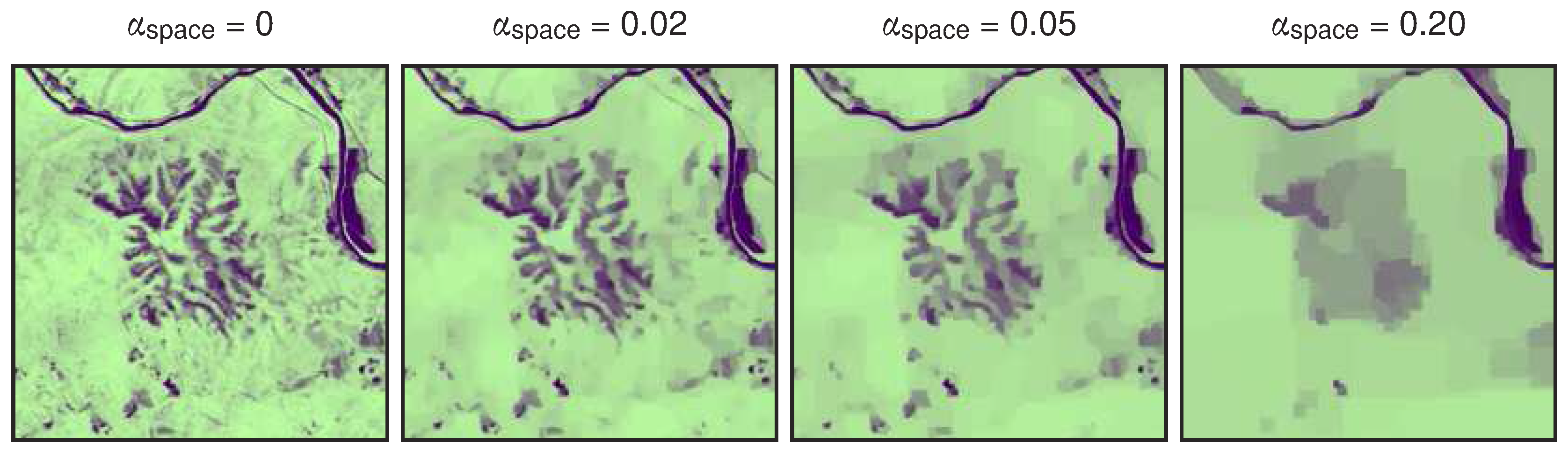
where are p-norms, ∇ is the gradient operator, is the composite vegetation index image, is a proposed solution, and controls the trade off between fidelity to the original composite image and intensity of denoising. Low values of preserve most image features while removing small-scale heterogeneity; higher values create larger patches that tie together more of the landscape (Figure 3). Change detection is sensitive to the choice of this scale parameter. Too little denoising fails to tie together similar land cover and too much risks obscuring real fine-scale change. Future work that applies these methods using multiple values could be useful for detecting disturbance events at different spatial scales.
At this stage, patches can be identified in each composite as same-valued regions and aggregated, converted to vector layers, or left as the original raster structure. Our approach chooses the latter option for simplicity, at the expense of calculating the same temporal segmentation solution multiple times for pixels that share the same patch history.
2.2.7. Temporal Segmentation to Identify Events
Disturbances in forests and other ecosystems include events that are sudden, acute processes, such as landslides or fires, and events that are protracted over many years, such as damage from pollution or insect outbreaks. General purpose detection algorithms should detect both kinds of events and also provide information on when, how long, and at what intensity these events occurred. The model employed here conceives of forest change as a series of temporally non-overlapping periods of disturbance, stability, or regeneration. Each period is defined as the line segment between two break points in the vegetation index time series; the severity of the change is defined as the slope of the segment.
Like the construction of spatial patches, this too is a signal segmentation problem with the goal of producing homogeneous regions from a noisy signal. As in the spatial segmentation, TVR can be used for this problem. However, unlike in the spatial segmentation, instead of producing periods of constant value in a vegetation index (all of which we would define as ‘stable’), the temporal segmentation should produce periods of constant slope. One approach is to apply a derivative to the time series before using TVR for segmentation; however, numerical differentiation is unstable and the signal is easily lost to the noise. Instead, we find a solution, , to a modification of TVR where the integral of is compared to the original signal in the fidelity term:
where are p-norms, is a pixel-wise time series through vegetation index patches, is a proposed derivative of over time, is the analogue to and controls the tradeoff between fidelity to the original time series and the simplicity of the fitted time series (Figure 4), is the year-wise change in adjacent values of (and therefore the second-derivative of the resulting fitted time series), and is a T × T integration matrix, where T is the number of years in the time series:
By comparing an integrated to the original data in the fidelity term, the minimization procedure finds a that approximates the first derivative of ; integrating then generates a smoothed approximation of the original time series in a numerically stable way.
The power of TVR for segmentation comes from using an norm in the regularization term. The minimization is driven to a solution with a sparse ; that is, most second derivatives of the fitted time series will be zero, with some terms being non-zero. By extension, that implies will be composed of a series of same-valued runs with jumps in value between runs. And since represents a derivative, this means that the integrated approximation will be composed of a series of line segments of same-valued slope; that is, a piecewise linear representation.
For efficient convergence, this functional is minimized using the fixed point lagged diffusivity method [48], a standard method in numerical optimization for non-differentiable problems such as TVR.
Although this algorithm provides an approximate piecewise linear function, the output has two drawbacks. First, solutions have a smaller range of values than the original data. This is because small errors in the data fidelity term are made up for by reducing the size of jumps in the regularization term. Second, when is small, additional breakpoints can be introduced representing small changes in the slope. To combat both of these problems, a clean-up step is performed on the output to remove breakpoints with small changes in slope. Then, a piece-wise linear regression is applied such that each segment defined by the remaining breakpoints is simultaneously fit to the data. This clean-up relies on two parameters: one to scale the relationship between time and vegetation index in order to calculate an angle (), and one to define which angles are considered ‘small’ ().
A Note on TVR and Choosing and :
The values of the regularization terms and control the balance between the data fidelity and the smoothing term in both segmentations. Very low values cause the solution to simply equal the data, or its forward-difference in the linear fitting. Very high values cause the solution to tend toward a single patch that equals the mean of the image in the spatial problem or a simple linear regression for the temporal signal. The best value, in the sense that it optimally solves the ill-posed inverse problem , is obtained by setting the respective equal to the magnitude of the noise processes that ‘contaminate’ the data, . Empirically, as the signal-to-noise ratio approaches one, values of should increase to around twice this magnitude, or 2. Since vegetation indices are scaled between zero and one, this theoretical noise process will always have a magnitude of less than one and, for most imagery, usually 0.01 to 0.10. However, it can never be directly known.
2.2.8. Calculate Time Series Statistics
For each pixel, three distribution statistics over the simplified time series were calculated to represent dynamic process of disturbances and regeneration in a static spatial representation. First, the mean absolute change gives a measure of total volatility through time, with stable regions having low values and areas with repeated cycles of disturbance and regeneration being high; Secondly, skewness provides a measure of the overall pattern of disturbance or regeneration, with negative skew in predominantly disturbed areas and positive skew where years of regeneration were more frequent; Finally, an overall measure of forestedness was calculated as the 95th percentile of NDMI values (second highest value in our 27-year time series).
For visualization, these statistics can be mapped to hue, saturation, and brightness to create a changescape, which is a single image capturing the amount, direction and nature of disturbance over a landscape’s satellite observation record. The skew was mapped to hue such that predominantly disturbed areas are red and regenerating areas are blue, the 95th percentile of NDMI was mapped to saturation such that vegetated areas are more colorful and non-vegetated areas are grey or white, and the mean absolute change was mapped to brightness such that areas with more change are darker and stable areas are lighter.
2.3. Parameter Calibration
Appropriate parameter values for effective estimation of change in eastern forests are not obvious a priori and must be discovered empirically. A grid search was used to evaluate performance over a range of values for four parameters: the spatial and temporal regularization terms ( and ), and the two temporal-segmentation simplification parameters ( and ). These parameter explorations were performed for each of the four vegetation indices: NDMI, NBR, TCA, and NDVI.
Trends in forest change were generated for each combination of vegetation index and parameters and then compared to manual interpretations of disturbance, stability, and regeneration in 155 forested plots corresponding to Landsat pixels in the study area. Pixels for manual classification were selected from a calibration region (Figure 1) via stratified sampling. Fifteen pixels with NDVI values greater than 0.6 at least two years in the time series were selected for each of the twelve tiles in the calibration region. Twenty-five were determined by the human interpreter to have never been forested and were excluded. Manual classification was performed by an independent interpreter with knowledge of eastern forest processes using the TimeSync application [49]. TimeSync allows the interpreter to select start and end dates of disturbed, regenerating, and stable periods, and then label those events with presumed causal agent, severity, and other attributes. While determining dates and attributes, the interpreter incorporates other data sources such as Google Earth imagery, Insect and Disease Survey data, and their own expert knowledge. In total, 4185 samples were used in calibration, with each representing an interpretation at each plot and year.
The total change over a VeRDET segment is a continuous-valued parameter. Comparing it to the discrete classification from the manual interpretation requires two thresholds near zero to delineate the positive and negative bounds of the ‘stable’ class. To minimize the effect of thresholding when assessing the parameters of interest, these values were chosen empirically to best fit the data, while constraining the threshold between ‘disturbance’ and ‘stability’ to be less than zero and the threshold between ‘stability’ and ‘regeneration’ to be greater than zero.
Cohen’s kappa, a metric of agreement [50], was then calculated between the determinations from each parameter combination and the manual determinations. Since optimal parameter values are expected to be different for vegetation indices with different effective ranges, kappa values were aggregated and compared within each vegetation index using a nested design.
2.4. Classification Evaluation
An additional 1183 TimeSync interpretations were made available from the North American Forest Dynamics (NAFD) project [2] and used here to evaluate VeRDET for its detection accuracy over the entire study region. These additional data included interpretations of disturbance type, allowing for accuracy to be evaluated by agent. Interpretations of ‘stable’ and ‘regenerating’ were used directly in the evaluation, while interpretations indicating physiological stress, wind and storm damage, wildfire, mechanical removal, harvest, and post-harvest site preparation fire were counted together generically as disturbance events. Interpretations pertaining to agriculture, natural thinning, and species composition change were omitted, as were years where locations were non-forested, which sometimes changed over the course of the time series. Overall, 20,283 samples, each representing an interpretation at each plot and year, were used in the evaluation. Of those, 509 represent disturbance.
Annual change rates were derived by summing disturbance and regeneration by year and then dividing by the total forested area within each ecoregion. The forest mask was defined using logistic regression of the 95th percentile NDMI against pixels labeled as forested in the TimeSync dataset. This allowed all areas ever forested within the time series to be included.
3. Results
3.1. Parameter Calibration
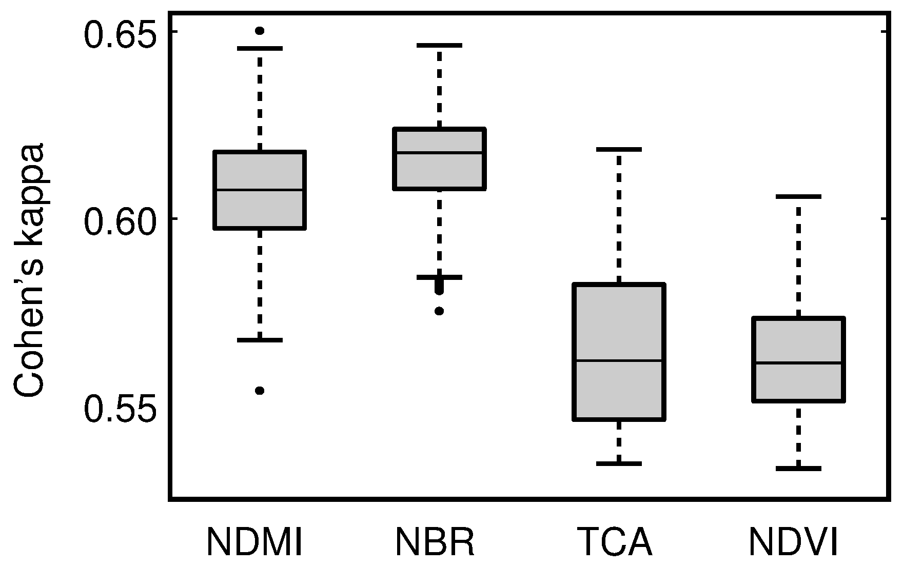
VeRDET was tested using multiple vegetation indices: the normalized difference vegetation index (NDVI), normalized burn ratio (NBR), tasseled cap angle (TCA), and normalized difference moisture index (NDMI), and different values for the spatial and temporal averaging. Over all parameter combinations, NDMI and NBR performed better than TCA and NDVI, with the best NDMI and NBR combinations producing Cohen’s kappas near 0.65, the best TCA combination producing kappas near 0.63, and the best NDVI combination giving kappa near 0.61. Some very poor-performing TCA and NDVI combinations give kappas of 0.53 (Figure 5). Results using NBR have lower variation than those using other vegetation indices, suggesting it is less sensitive to parameter value selections.
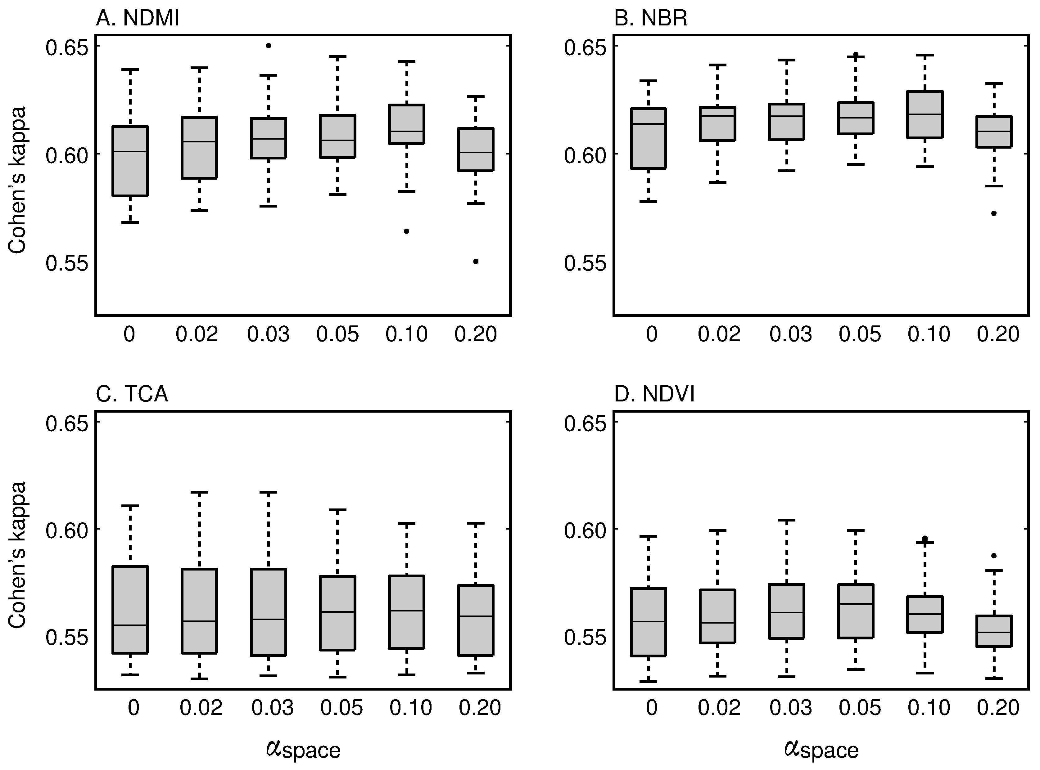
We evaluated performance over a range of values for from 0, representing the most detailed imagery and no patch creation, through 0.20, representing larger patches with little detail. The highest kappas (represented by the upper bounds in Figure 6) were generated using moderate spatial aggregation. Values of around 0.03 or 0.05 for perform best, with somewhat larger values (less detail, larger patches) preferred for NDMI and NBR and smaller values (more detail, smaller patches) for TCA and NDVI.
Performance was evaluated for a range of from 0.01, resulting in very little regularization and high fidelity to the noisy time series, to 0.20, resulting in large amounts of temporal smoothing. Variation in represents the majority of the variation in algorithm performance for all vegetation indices (Figure 7). For NDMI and NBR, the best estimates of change in eastern forest are produced using values for of around 0.03. For TCA and NDVI, values of that preserve less of the underlying time series produce the best results, with values around 0.10 being optimal, suggesting that change signals derived from those indices are noisier through time than signals derived from indices that use shortwave infrared bands.
Two other potentially tunable parameters were explored: the ratio between the vegetation index and years () and the angle threshold for temporal simplification (). Five values were tested for both and ranging from 0.001 to 0.025. Both parameters were statistically significant due to the large number of samples, but the effect sizes were very small compared to the spatial and temporal fidelity terms. Graphical results for these parameters are presented in Supplementary Materials Figures S1 and S2.
3.2. Interaction between Temporal Fidelity and Classification Thresholds
Temporal segmentation using TVR removes information from the time series and smooths out noise. One way to assess whether this information is really noise, as opposed to an ecological process of interest, is to examine how optimal thresholds discriminating between change and stability differ under different regularization strengths (Figure 8). If TVR removes an equal amount of information about disturbance as it does noise, then the optimal discrimination thresholds should be consistent for different levels of regularization. Instead, with increased regularization (more smoothing) those thresholds approach zero, meaning that actually stable segments have very small change magnitudes associated with them and actual change segments have larger change magnitudes. That is, at least over the range of parameters explored, increased regularization enables more precise discrimination between change and non-change events. This allows the algorithm to be sensitive and correctly identify weaker disturbances associated with forest stress or slow re-greenings.
3.3. Classification Evaluation
The parameter set using NDMI as the basis for segmentation with parameters = 0.03, = 0.03, = 0.025, = 0.01, performed best within the calibration region and was chosen for change detection over the entire study area. Segments were labeled ‘stable’ if the absolute total change over the segment was less than 0.055 in NDMI; segments with a greater negative change were labeled ‘disturbed’ and those with a greater positive change were labeled ‘regenerating’.
Agreement with the NAFD dataset is shown in Table 1. VeRDET performed well in detecting large, fast disturbances such as fires, mechanical disruption, and harvest events with omission errors ranging from 22.2% to 36.7%, but struggled to distinguish physiological stress from a stable condition, omitting 77.8%. Overall omission error for all disturbances is 38.3% and commission error is 74.0%. VeRDET accurately characterizes stable regions, with omission error of 19.8% and commission error of 28.1%. Growing areas were labeled as stable about half the time, most often because the regeneration label was extended in the TimeSync data well after the spectral response had recovered, highlighting a fundamental obstacle in forest monitoring from remotely sensed imagery.
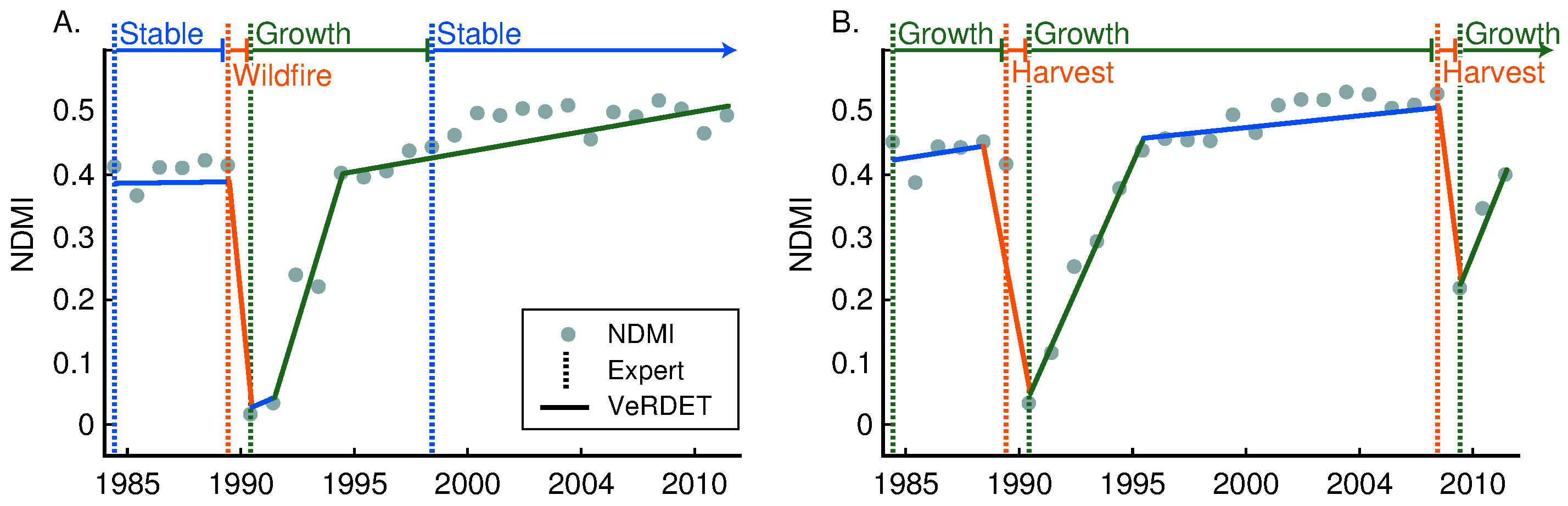
Visually, time-series segmentations from both VeRDET and the expert interpretation coincide well in forested patches with significant disturbance events (Figure 9). VeRDET segmentations often add short periods of stability whereas the expert often chooses one year as a breakpoint. This may be due to VeRDET having insufficient imagery during those years and thus the weighted averaging is interpreted as stability, whereas the expert had access to additional data sources and imagery dates and can therefore make an informed decision. Additionally, some incorrectly identified breakpoints occur a year before or after the expert identified years. Effectively, the disturbance events are detected but start and end points are imprecisely defined, potentially from insufficient imagery or the discretization of a continuous time series.
Allowing VeRDET breakpoints to ‘snap’ to the expert-identified breakpoints within a tolerance of year can provide insight into how much error is from missing change events versus temporal imprecision. Doing so, the overall error decreased from 32.0% to 26.5% (Table 2); error of omission for all disturbances decreased from 38.3% to 33.4%, and commission errors for all disturbances decreased from 74.0% to 62.9%. Notably, approximately 10% more regenerating years were correctly identified. These error reductions are similar to those found in other studies performing the same procedure [36].
3.4. Spatial and Temporal Patterns of Change
For most of the Eastern United States, forests are stable or regenerating (Figure 10). The different ecoregions in the study region, however, exhibit differences in both spatial and temporal (Figure 11) patterns of change. The Western Allegheny Plateau is primarily covered by stable forests (light green) in northeastern West Virginia, with the bulk of disturbance (red) and mixed forest change (green) detected in southern Ohio and western Pennsylvania (Figure 10). A peak in the amount of the disturbance in this ecoregion occurred in 1988 and again in 1998, and both peaks are followed by increases in the percent area undergoing regeneration (Figure 11).
The North Central Appalachians (B) and Central Appalachians (C) have a mixture of stable forests (light green) punctuated with large regions of severe disturbance (red) (Figure 10). In the North Central Appalachians, this disturbance occurred prior to 1994, and is followed by a large amount of regeneration. In the Central Appalachians, peaks in forest area disturbed occurred in the late 1980s, late 1990s, and mid 2000s (Figure 11). Also notable in these regions are two large areas of intense regrowth (blue) representing forest response to large disturbances that predate the time series (Figure 10).
The patterns of change in the Ridge and Valley (D) reflect the topography of this region, with mixed change occurring in the valleys, and relatively stable forests along the ridges; the bulk of the disturbance in this region occurs at the southern end (Figure 10). The temporal pattern in disturbed area is the most regular here, with peaks occurring every 5 to 7 years (Figure 11). The least amount of forest change was observed in the Blue Ridge (E), and most of this change occurs in the northern and southern edges of the region (Figure 10). Relatively little forest area is affected throughout all years in the study period (Figure 11).
Most forest disturbance (red) in the study area occurs in the Piedmont (F) (Figure 10). Nearly all areas in this ecoregion are also affected by regular forest change (dark green). Both of these patterns are supported by the much higher affected forest area through all years in the study period (Figure 11).
4. Discussion
VeRDET allows the shifting mosaic of forest stand dynamics to emerge from the data with minimal human input. VeRDET can identify years of fast and slow disturbance, stability, and regeneration in complex eastern forests. A recent comparison of disturbance detection algorithms by Cohen et al. included an earlier version of VeRDET, where it compared favorably with established algorithms such as LandTrendr and CCDC with similar overall errors [36]. Omission and commission rates of VeRDET were balanced, representing the middle of the tradeoff curve between error types, with lower omission rates than CCDC and lower commission rates than LandTrendr. Additionally, VeRDET had the most accurate estimates of percent forest area disturbed through time, likely due to its balanced error structure. These results also speak to VeRDET’s generality, as the study region in Cohen et al. and the one in this study are disjointed. The improvements in omission error seen here can be attributed to evaluating VeRDET against the ecosystems for which it was developed, the lower amount of low-intensity ‘stress’ in this study region, and a number of minor algorithm improvements.
Several sources of error exist. VeRDET will often begin a disturbance segment a year earlier or end it a year later than the human interpreter, most likely due to noise in the time series, missing dates, or from discretization inherent in creating yearly composites. Additionally, pixels on the edges of patches, of which there are very many in fragmented eastern forests [51] are often included into a patch with different dynamics than what was interpreted for the pixel. In extreme cases an edge pixel is alternatingly included in neighboring patches, making its time series unrepresentative of the actual dynamics for the location. Combining the patch-creation and temporal segmentation steps into a single pass could solve this problem. Finally, assessing agreement requires classifying a continuous variable of change into bins representing disturbance, stability, and regrowth, which we mitigate to some extent by fitting those thresholds. Still, the difference between a gradual forest stress and stability is likely different for different forest compositions and environments, and single thresholds are not likely to be adequate for large mapping projects.
Different vegetation indices relate to different ecologically relevant information, such as above ground biomass, forest density [52], and canopy chlorophyll content [53], and account for particular site-specific conditions [54]. In our comparison of VeRDET’s performance across different vegetation indices, the high performance of NDMI may be explained in part by its sensitivity to biomass [45], which may enable it to detect actual disturbances and to track regenerating biomass instead of just initial, rapid regreening from forbs. Cohen [49] also found that tasseled-cap wetness, an index that is informationally similar to NDMI and is believed to provide information on forest structure, performed better than other indices. Although the use of NDMI or wetness for vegetation studies is less common than NDVI or NBR, these indices are promising indicators of disturbance and should be included in future forest disturbance studies.
Our model of forest disturbance is patch-based, that is, patches are the unit over which the processes of forest disturbance and regeneration operate, and patch size matters with regard to different disturbance agents, for instance different burn intervals and severity [55]. The approach presented here creates patches of forest change in space and time, rather than aggregating pixel level changes in a post-processing step. Sensitivity analysis presented here shows that a moderate level of patch size and detail best matches expert interpretation. While too much regularization removes the fine-level detail needed to match expert interpretation, too little regularization overemphasizes pixel-level noise and sub-patch processes. The same pattern also appears, but stronger, in temporal regularization. The time-series is noisy and so some level of smoothing is required to account for phenology and atmospheric differences between yearly composites. However, additionally, the temporal regularization enforces our conceptual model of forest change as a series of disturbed, stable, and regeneration periods by tying together years of progressive ecological change, even when some years in the middle of the process may have momentarily re-greened or appeared stable spectrally.
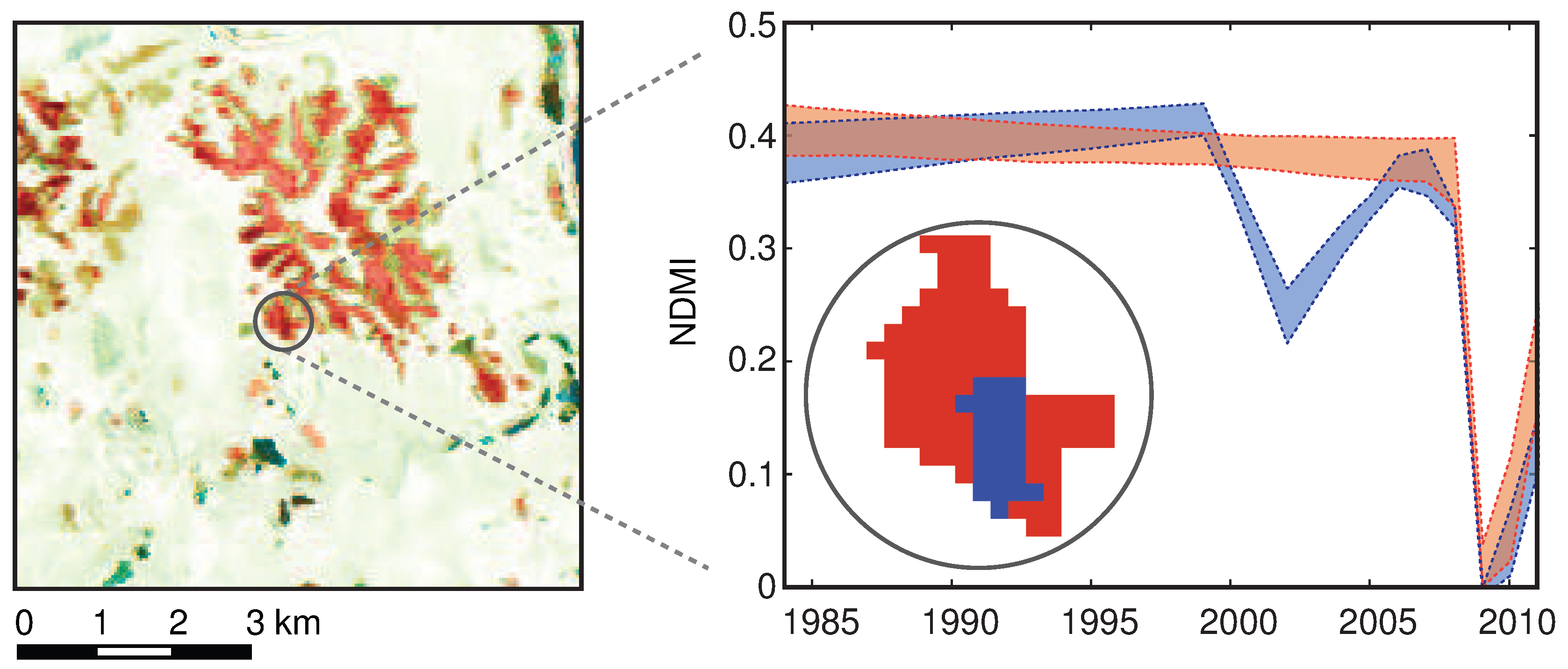
Because patches are discrete in space and time, and because disturbance events are not independent of one another, patches may overlap. For instance, drought and southern pine beetle increase pine tree mortality, which then increases the likelihood of fire in heavily-infested pine-dominated forests. This example is illustrated at a site of a known pine beetle outbreak (blue) which then burned in 2009 (red) (Figure 12). The insect outbreak decreases NDMI over a four year period early in the time series, the fire is a quick and intense disturbance event that occurs within the same area. The patches shown in Figure 12 are from 2010; because VeRDET creates patches in each yearly composite independent of the time series, pixels on patch edges can shift membership between neighboring patches through time and ephemeral patches can form within larger ones for some years, an extreme example being the insect outbreak shown. Because of this the temporal trajectories for each pixel within a patch in a given year are often slightly different and are shown here as band of similarly-behaving trajectories. A process that segments space and time simultaneously could resolve such ambiguities, but at a trade-off of computational expense and efficient parallelization.
When VeRDET was used to map change over the Eastern United States (Figure 10), the different ecoregions exhibited striking differences in the levels and spatial patterns of disturbance. These differences reflect common disturbance agents and management practices in each region. The Western Allegheny Plateau (A) encompasses a mixture of stable forests in West Virginia with traditional agriculture and ranching in southeastern Ohio and western Pennsylvania. The North Central Appalachians (B) and Central Appalachians (C) have a mixture of stable forests punctuated with large regions of severe disturbance, primarily from coal mines. The Ridge and Valley region (D) is stratified with forests on hilltops and agriculture in valleys. The agricultural areas have large amounts of inter-annual change, but no real trend due to human activity that periodically cuts fields to prevent them from succeeding to forest. The significant amount of regeneration seen in this area is likely due to old fields being allowed to transition to forest as agriculture and ranching become less economically important to the area. In addition, this area has substantial human development, indicated by the very geometrically regular pattern of clear cuts and regrowth. The striking stability in the Blue Ridge ecoregion (E) owes to its lack of accessibility and patchwork of protected areas including the Great Smoky Mountains National Park, the Nantahala, Chattahoochee, Pisgah, and Cherokee National Forests, and other wilderness areas managed to prevent land cover conversion [56]. Disturbed sections in the northern part of the Blue Ridge have strongly negative trends, likely caused by pine beetle dieoff that has subsequently burned. Disturbed sections in the southern part are primarily a result of tree mortality from a mixture of southern pine beetle and hemlock woolly adelgid. Other tree and shrub species in these forests have then filled in the post-disturbed areas, resulting in a mixed disturbance/regeneration trend in the map. Finally, the Piedmont (F) is characterized by intense human development and rotating timber harvesting.
Different disturbance detection methods are developed with different definitions of forest disturbance in mind, and therefore excel at identifying different landscape processes. VeRDET is flexible both in the spatial and temporal scale of the processes. Future work should focus on increasing flexibility of disturbance detection by combining outputs derived from different vegetation indices and from different values of and into an ensemble model. Additionally, combining spatial and temporal segmentation into a single, three-dimensional segmentation will enable the algorithm to identify forest change processes in the imagery stack. Information from these identified processes can then be extracted for further analysis, such as labeling change agent.
5. Conclusions
We developed and evaluated a new change detection method which uses a global segmentation algorithm, total variation regularization, to identify and track forest change using Landsat data. The method relies on two key parameters which can be interpreted as scaling factors in space and time. Our approach uses a conceptual model of forest change occurring in patches instead of pixels, and so identifies spatially similar regions in satellite imagery prior to change detection. This enables the identification of spatially-coherent change events within heterogeneous forests even when the spatial grain of imagery would normally result in the identification of many small, disconnected events. This patch-based approach may facilitate integration of imagery from sensors with differing spatial scales, such as the Multispectral Scanner or Sentinel-2.
Supplementary Materials
The following are available online at www.mdpi.com/1999-4907/8/5/166/s1, Figure S1: Kappa by , the ratio between vegetation index and years, Figure S2: Kappa by , the angle threshold for temporal simplification.
Acknowledgments
This research was supported through Grant NO. NNX10AT66G of the NASA New Investigator program and the Scalable Computing and Leading Edge Innovative Technologies (SCALE-IT) fellowship, part of the NSF’s Integrative Graduate Education and Research Traineeship program. We thank Lou Gross and Robert Kennedy, and three anonymous reviewers for their valuable comments on earlier drafts of this manuscript.
Author Contributions
M. Joseph Hughes and Daniel J. Hayes conceived and designed the project. M. Joseph Hughes developed VeRDET and analyzed data. S. Douglas Kaylor generated ground-truth data for model calibration. M. Joseph Hughes, S. Douglas Kaylor and Daniel J. Hayes wrote the manuscript.
Conflicts of Interest
The authors declare no conflict of interest.
References
- White, P.S.; Collings, B.S.; Wein, G.R. Natural disturbances and early successional habitats. In Sustaining Young Forest Communities; Greenberg, C.H., Collins, B.S., Thompson, F.R., Eds.; Springer: Dordrecht, The Netherlands, 2011; pp. 27–40. [Google Scholar]
- Goward, S.N.; Masek, J.G.; Cohen, W.; Moisen, G.; Collatz, G.J.; Healey, S.; Houghton, R.A.; Huang, C.; Kennedy, R.; Law, B.; et al. Forest disturbance and North American carbon flux. EOS Trans. Am. Geophys. Union 2008, 89, 105–116. [Google Scholar] [CrossRef]
- Williams, C.A.; Collatz, G.J.; Masek, J.; Huang, C.; Goward, S.N. Impacts of disturbance history on forest carbon stocks and fluxes: Merging satellite disturbance mapping with forest inventory data in a carbon cycle model framework. Remote Sens. Environ. 2014, 151, 57–71. [Google Scholar] [CrossRef]
- Bleby, T.M.; McElrone, A.J.; Jackson, R.B. Water uptake and hydraulic redistribution across large woody root systems to 20 m depth. Plant Cell Environ. 2010, 33, 2132–2148. [Google Scholar] [CrossRef] [PubMed]
- Pugh, E.; Gordon, E. A conceptual model of water yield effects from beetle-induced tree death in snow-dominated lodgepole pine forests. Hydrol. Process. 2013, 27, 2048–2060. [Google Scholar] [CrossRef]
- Aber, J.D.; Ollinger, S.V.; Driscoll, C.T.; Likens, G.E.; Holmes, R.T.; Freuder, R.J.; Goodale, C.L. Inorganic nitrogen losses from a forested ecosystem in response to physical, chemical, biotic, and climatic perturbations. Ecosystems 2002, 5, 648–658. [Google Scholar] [CrossRef]
- Bernal, S.; Hedin, L.O.; Likens, G.E.; Gerber, S.; Buso, D.C. Complex response of the forest nitrogen cycle to climate change. Proc. Natl. Acad. Sci. USA 2012, 109, 3406–3411. [Google Scholar] [CrossRef] [PubMed]
- Dale, V.H.; Joyce, L.A.; Mcnulty, S.; Neilson, R.P.; Ayres, M.P.; Flannigan, M.D.; Hanson, P.J.; Irland, L.C.; Lugo, A.E.; Peterson, C.J.; et al. Climate Change and Forest Disturbances. BioScience 2001, 51, 723–734. [Google Scholar] [CrossRef]
- Weed, A.S.; Ayers, M.P.; Hicke, J.A. Consequences of climate change for biotic disturbances in North American forests. Ecol. Monogr. 2013, 83, 441–470. [Google Scholar] [CrossRef]
- Pickett, S.T.A.; White, P.S. The Ecology of Natural Disturbance and Patch Dynamics; Academic Press: Orlando, FL, USA, 1985; Volume 1, p. 472. [Google Scholar]
- Masek, J.G.; Hayes, D.J.; Hughes, M.J.; Healey, S.P.; Turner, D.P. The role of remote sensing in process-scaling studies of managed forest ecosystems. For. Ecol. Manag. 2015, 355, 109–123. [Google Scholar] [CrossRef]
- Dale, V.H.; Hughes, M.J.; Hayes, D.J. Climate Change and the Future of Natural Disturbances in the Central Hardwood Region. In Natural Disturbances: Historic Range of Variation and Effects on Upland Hardwood Forest Structure in the Southeastern US; Greenberg, C.H., Collins, B.S., Eds.; Springer International: Cham, Switzerland, 2015; pp. 355–369. [Google Scholar]
- Kasischke, E.S.; Verbyla, D.L.; Rupp, T.S.; McGuire, A.D.; Murphy, K.A.; Jandt, R.; Barnes, J.L.; Hoy, E.E.; Duffy, P.A.; Calef, M.; et al. Alaska’s changing fire regime—Implications for the vulnerability of its boreal forests. Can. J. For. Res. 2010, 40, 1313–1324. [Google Scholar] [CrossRef]
- Coomes, D.A.; Holdaway, R.J.; Kobe, R.K.; Lines, E.R.; Allen, R.B. A general integrative framework for modelling woody biomass production and carbon sequestration rates in forests. J. Ecol. 2012, 100, 42–64. [Google Scholar] [CrossRef]
- Hayes, D.J.; McGuire, A.D.; Kicklighter, D.W.; Gurney, K.R.; Burnside, T.J.; Melillo, J.M. Is the northern high-latitude land-based CO2 sink weakening? Glob. Biogeochem. Cycles 2011, 25. [Google Scholar] [CrossRef]
- Medvigy, D.; Moorcroft, P.R. Predicting ecosystem dynamics at regional scales: An evaluation of a terrestrial biosphere model for the forests of northeastern North America. Philos. Trans. R. Soc. B Biol. Sci. 2012, 367, 222–235. [Google Scholar] [CrossRef] [PubMed]
- Smith, M.J.; Vanderwel, M.C.; Lyutsarev, V.; Emmott, S.; Purves, D.W. The climate dependence of the terrestrial carbon cycle; including parameter and structural uncertainties. Biogeosci. Discuss. 2012, 9, 13439–13496. [Google Scholar] [CrossRef]
- Kennedy, R.E.; Andréfouët, S.; Cohen, W.B.; Gómez, C.; Griffiths, P.; Hais, M.; Healey, S.P.; Helmer, E.H.; Hostert, P.; Lyons, M.B.; et al. Bringing an ecological view of change to landsat-based remote sensing. Front. Ecol. Environ. 2014, 12, 339–346. [Google Scholar] [CrossRef]
- Masek, J.G.; Huang, C.; Wolfe, R.; Cohen, W.; Hall, F.; Kutler, J.; Nelson, P. North American forest disturbance mapped from a decadal Landsat record. Remote Sens. Environ. 2008, 112, 2914–2926. [Google Scholar] [CrossRef]
- Wilson, E.H.; Sader, S.A. Detection of forest harvest type using multiple dates of Landsat TM imagery. Remote Sens. Environ. 2002, 80, 385–396. [Google Scholar] [CrossRef]
- García-Haro, F.J.; Gilabert, M.A.; Meliá, J. Monitoring fire-affected areas using Thematic Mapper data. Int. J. Remote Sens. 2001, 22, 533–549. [Google Scholar] [CrossRef]
- Lu, D.; Weng, Q. A survey of image classification methods and techniques for improving classification performance. Int. J. Remote Sens. 2007, 28, 823–870. [Google Scholar] [CrossRef]
- Woodcock, C.E.; Allen, R.; Anderson, M.; Belward, A.; Bindschadler, R.; Cohen, W.; Gao, F.; Goward, S.N.; Helder, D.; Helmer, E.; et al. Free access to Landsat imagery. Science 2008, 320, 1011. [Google Scholar] [CrossRef] [PubMed]
- Vogelmann, J.E.; Tolk, B.; Zhu, Z. Monitoring forest changes in the southwestern United States using multitemporal Landsat data. Remote Sens. Environ. 2009, 113, 1739–1748. [Google Scholar] [CrossRef]
- Zhao, C.; Hobbs, B.E.; Ord, A. Fundamentals of computational geoscience: Numerical methods and algorithms. Lect. Notes Earth Sci. 2009, 122, 1–257. [Google Scholar]
- Brooks, E.B.; Wynne, R.H.; Thomas, V.A.; Blinn, C.E.; Coulston, J.W. On-the-Fly Massively Multitemporal Change Detection Using Statistiacl Quality Control Charts and Landsat Data. IEEE Trans. Geosci. Remote Sens. 2014, 52, 3316–3332. [Google Scholar] [CrossRef]
- Jamali, S.; Jönsson, P.; Eklundh, L.; Ardö, J.; Seaquist, J. Detecting changes in vegetation trends using time series segmentation. Remote Sens. Environ. 2015, 156, 182–195. [Google Scholar] [CrossRef]
- Huang, C.; Thomas, N.; Goward, S.N.; Masek, J.G.; Zhu, Z.; Townshend, J.R.G.; Vogelmann, J.E. Automated masking of cloud and cloud shadow for forest change analysis using Landsat images. Int. J. Remote Sens. 2010, 31, 5449–5464. [Google Scholar] [CrossRef]
- Kennedy, R.E.; Yang, Z.; Cohen, W.B. Detecting trends in forest disturbance and recovery using yearly Landsat time series: 1. LandTrendr—Temporal segmentation algorithms. Remote Sens. Environ. 2010, 114, 2897–2910. [Google Scholar] [CrossRef]
- Hermosilla, T.; Wulder, M.A.; White, J.C.; Coops, N.C.; Hobart, G.W. An integrated Landsat time series protocol for change detection and generation of annual gap-free surface reflectance composites. Remote Sens. Environ. 2015, 158, 220–234. [Google Scholar] [CrossRef]
- Hermosilla, T.; Wulder, M.A.; White, J.C.; Coops, N.C.; Hobart, G.W.; Campbell, L.B. Mass data processing of time series Landsat imagery: Pixels to data products for forest monitoring. Int. J. Digit. Earth 2016, 9. [Google Scholar] [CrossRef]
- Zhu, Z.; Woodcock, C.E.; Olofsson, P. Continuous monitoring of forest disturbance using all available Landsat imagery. Remote Sens. Environ. 2012, 122, 75–91. [Google Scholar] [CrossRef]
- Hughes, M.; Hayes, D. Automated detection of cloud and cloud shadow in single-date Landsat imagery using neural networks and spatial post-processing. Remote Sens. 2014, 6, 4907–4926. [Google Scholar] [CrossRef]
- Zhu, Z.; Woodcock, C.E. Object-based cloud and cloud shadow detection in Landsat imagery. Remote Sens. Environ. 2012, 118, 83–94. [Google Scholar] [CrossRef]
- Schwarz, G. Estimating the dimension of a model. Ann. Stat. 1978, 6, 461–464. [Google Scholar] [CrossRef]
- Cohen, W.B.; Healey, S.P.; Yang, Z.; Stehman, S.V.; Brewer, C.K.; Brooks, E.B.; Gorelick, N.; Huang, C.; Hughes, M.J.; Kennedy, R.E.; et al. How Similar Are Forest Disturbance Maps Derived from Different Landsat Time Series Algorithms? Forests 2017, 8, 98. [Google Scholar] [CrossRef]
- Oliver, C.D.; Larson, B.C. Forest Stand Dynamics; Updated Edition; John Wiley and Sons: Hoboken, NJ, USA; 1996. [Google Scholar]
- Omernik, J. Ecoregions of the conterminous United States. Map (scale 1:7,500,000). Ann. Assoc. Am. Geogr. 1987, 77, 118–125. [Google Scholar] [CrossRef]
- Chander, G.; Markham, B.L.; Helder, D.L. Summary of current radiometric calibration coefficients for Landsat MSS, TM, ETM+, and EO-1 ALI sensors. Remote Sens. Environ. 2009, 113, 893–903. [Google Scholar] [CrossRef]
- Chavez, P.S. An improved dark-object subtraction technique for atmospheric scattering correction of multispectral data. Remote Sens. Environ. 1988, 24, 459–479. [Google Scholar] [CrossRef]
- Chavez, P.S. Image-based atmospheric corrections—Revisited and improved. Photogramm. Eng. Remote Sens. 1996, 62, 1025–1036. [Google Scholar]
- Powell, S.L.; Cohen, W.B.; Healey, S.P.; Kennedy, R.E.; Moisen, G.G.; Pierce, K.B.; Ohmann, J.L. Quantification of live aboveground forest biomass dynamics with Landsat time-series and field inventory data: A comparison of empirical modeling approaches. Remote Sens. Environ. 2010, 114, 1053–1068. [Google Scholar] [CrossRef]
- Tucker, C.J. Red and photographic infrared linear combinations for monitoring vegetation. Remote Sens. Environ. 1979, 8, 127–150. [Google Scholar] [CrossRef]
- Van Wagtendonk, J.W.; Root, R.R.; Key, C.H. Comparison of AVIRIS and Landsat ETM+ detection capabilities for burn severity. Remote Sens. Environ. 2004, 92, 397–408. [Google Scholar] [CrossRef]
- Jin, S.; Sader, S.A. Comparison of time series tasseled cap wetness and the normalized difference moisture index in detecting forest disturbances. Remote Sens. Environ. 2005, 94, 364–372. [Google Scholar] [CrossRef]
- Rudin, L.; Osher, S.; Fatemi, E. Nonlinear total variation based noise removal algorithms. Phys. D Nonlinear Phenom. 1992, 60, 259–268. [Google Scholar] [CrossRef]
- Goldstein, T.; Osher, S. The split Bregman method for L1-regularized problems. SIAM J. Imaging Sci. 2009, 2, 323–343. [Google Scholar] [CrossRef]
- Vogel, C.R.; Oman, M.E. Iterative methods for total variation denoising. SIAM J. Sci. Comput. 1996, 17, 227–238. [Google Scholar] [CrossRef]
- Cohen, W.B.; Yang, Z.; Kennedy, R.E. Detecting trends in forest disturbance and recovery using yearly Landsat time series: 2. TimeSync—Tools for calibration and validation. Remote Sens. Environ. 2010, 114, 2911–2924. [Google Scholar] [CrossRef]
- Cohen, J. A coefficient of agreement for nominal scales. Educ. Psychol. Meas. 1960, 20, 37–46. [Google Scholar] [CrossRef]
- Heilman, G.E., Jr.; Strittholt, J.R.; Slosser, N.C.; Dellasala, D.A. Forest fragmentation of the conterminous United States: Assessing forest intactness through road density and spatial characteristics. Bioscience 2002, 52, 411–422. [Google Scholar] [CrossRef]
- Gómez, C.; White, J.C.; Wulder, M.A.; Alejandro, P. Historical forest biomass dynamics modelled with Landsat spectral trajectories. ISPRS J. Photogramm. Remote Sens. 2014, 93, 14–28. [Google Scholar] [CrossRef]
- Gamon, J.A.; Field, C.B.; Goulden, M.L.; Griffin, K.L.; Hartley, A.E.; Joel, G.; Penuelas, J.; Valentini, R. Relationships between NDVI, canopy structure, and photosynthesis in three Californian vegetation types. Ecol. Appl. 1995, 5, 28–41. [Google Scholar] [CrossRef]
- Lozano, F.J.; Suárez-Seoane, S.; de Luis, E. Assessment of several spectral indices derived from multi-temporal Landsat data for fire occurrence probability modelling. Remote Sens. Environ. 2007, 107, 533–544. [Google Scholar] [CrossRef]
- Lozano, F.J.; Surez-Seoane, S.; De Luis-Calabuig, E. Does fire regime affect both temporal patterns and drivers of vegetation recovery in a resilient Mediterranean landscape? A remote sensing approach at two observation levels. Int. J. Wildl. Fire 2012, 21, 666–679. [Google Scholar] [CrossRef]
- U.S. Geological Survey, Gap Analysis Program. Protected Areas Database of the United States (PAD-US), Version 1.4 Combined Feature Class 2016. Available online: https://gapanalysis.usgs.gov/padus/ (accessed on 10 April 2017).
Figure 1.
Study area showing ecoregions of interest in the Eastern United States and the subset calibration region within which model parameters were determined.
Figure 1.
Study area showing ecoregions of interest in the Eastern United States and the subset calibration region within which model parameters were determined.
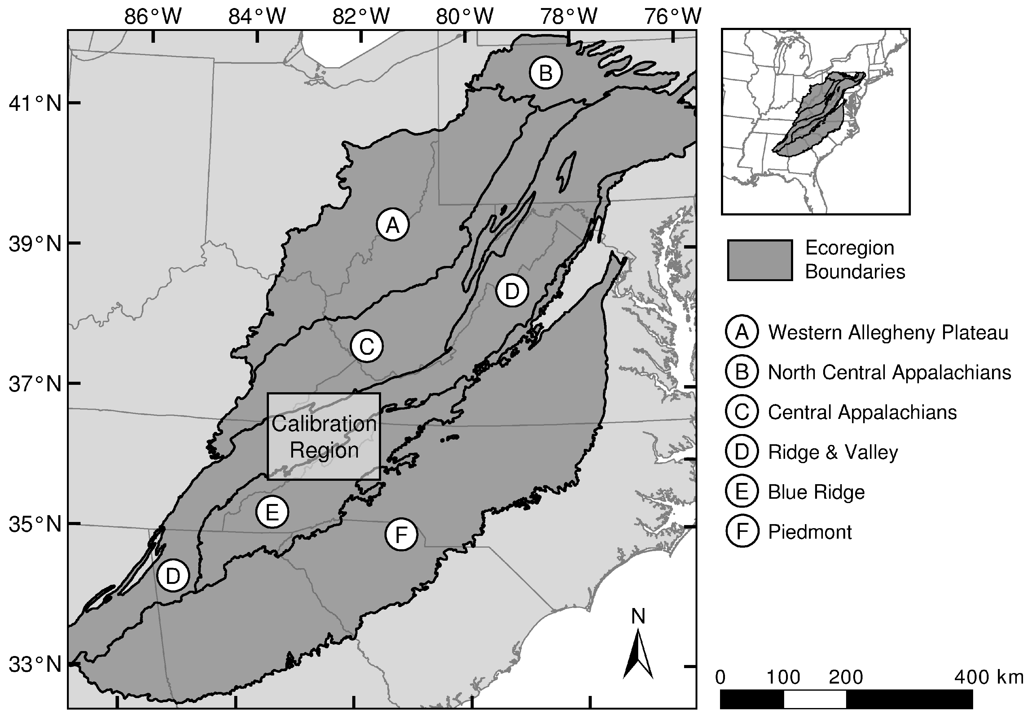
Figure 2.
Schematic of VeRDET pro- cessing steps to identify years and locations of forest change. TVR: total variation regularization.
Figure 2.
Schematic of VeRDET pro- cessing steps to identify years and locations of forest change. TVR: total variation regularization.
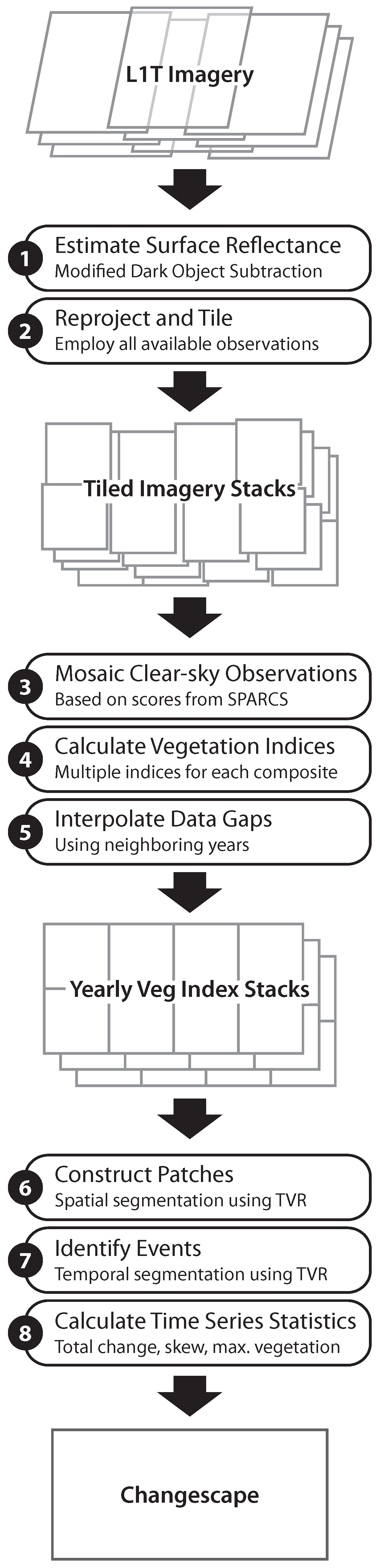
Figure 3.
Two-dimential total variation regularization over a false color vegetation index near a wildfire. Low values of preserve more small-scale features while high values incorporate local heterogeneity into uniform patches.
Figure 3.
Two-dimential total variation regularization over a false color vegetation index near a wildfire. Low values of preserve more small-scale features while high values incorporate local heterogeneity into uniform patches.

Figure 4.
Total variation regularization over the time series generates many quick events or fewer, longer-term events depending on the strength of .
Figure 4.
Total variation regularization over the time series generates many quick events or fewer, longer-term events depending on the strength of .
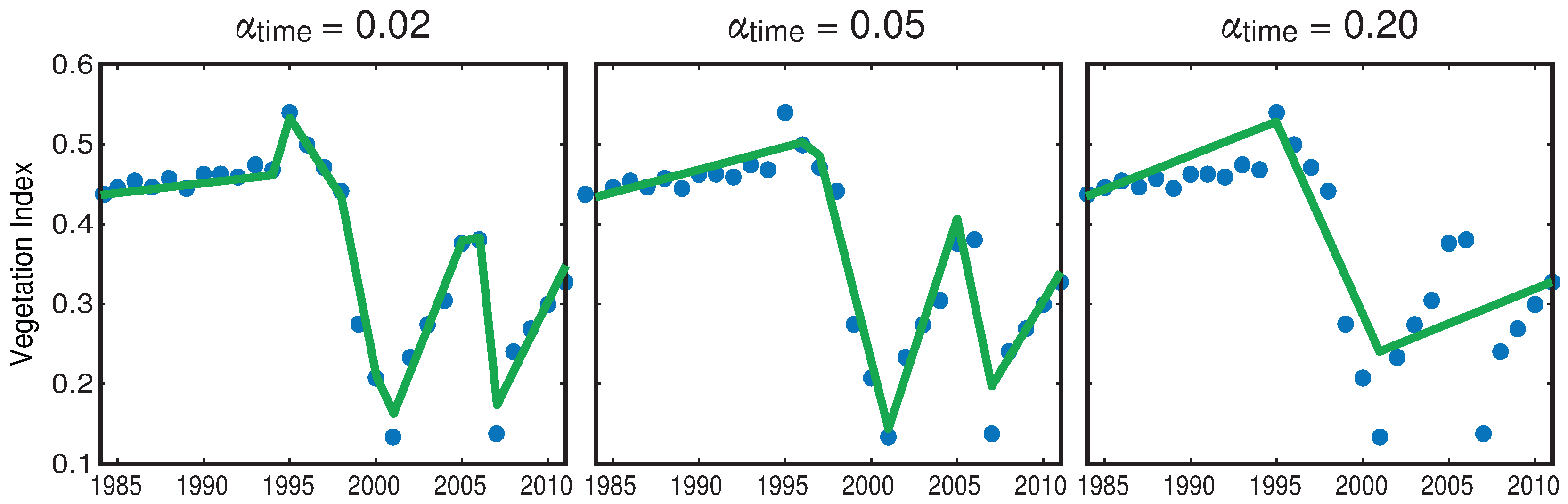
Figure 5.
Range of Cohen’s kappa over all parameter combinations for four different vegetation indices.
Figure 5.
Range of Cohen’s kappa over all parameter combinations for four different vegetation indices.

Figure 6.
Effect of the strength of the spatial fidelity parameter on performance (kappa) within each vegetation index (A–D). Higher values of represent larger patches and less fidelity to the yearly composite images; zero represents no patch aggregation and complete fidelity to the composite images.

Figure 7.
Effect of the strength of the temporal fidelity parameter on performance (kappa) within each vegetation index (A–D). Higher values of represent less fidelity to the original time series and longer segments. Lower values represent a closer tracking of the time series and shorter segments.
Figure 7.
Effect of the strength of the temporal fidelity parameter on performance (kappa) within each vegetation index (A–D). Higher values of represent less fidelity to the original time series and longer segments. Lower values represent a closer tracking of the time series and shorter segments.
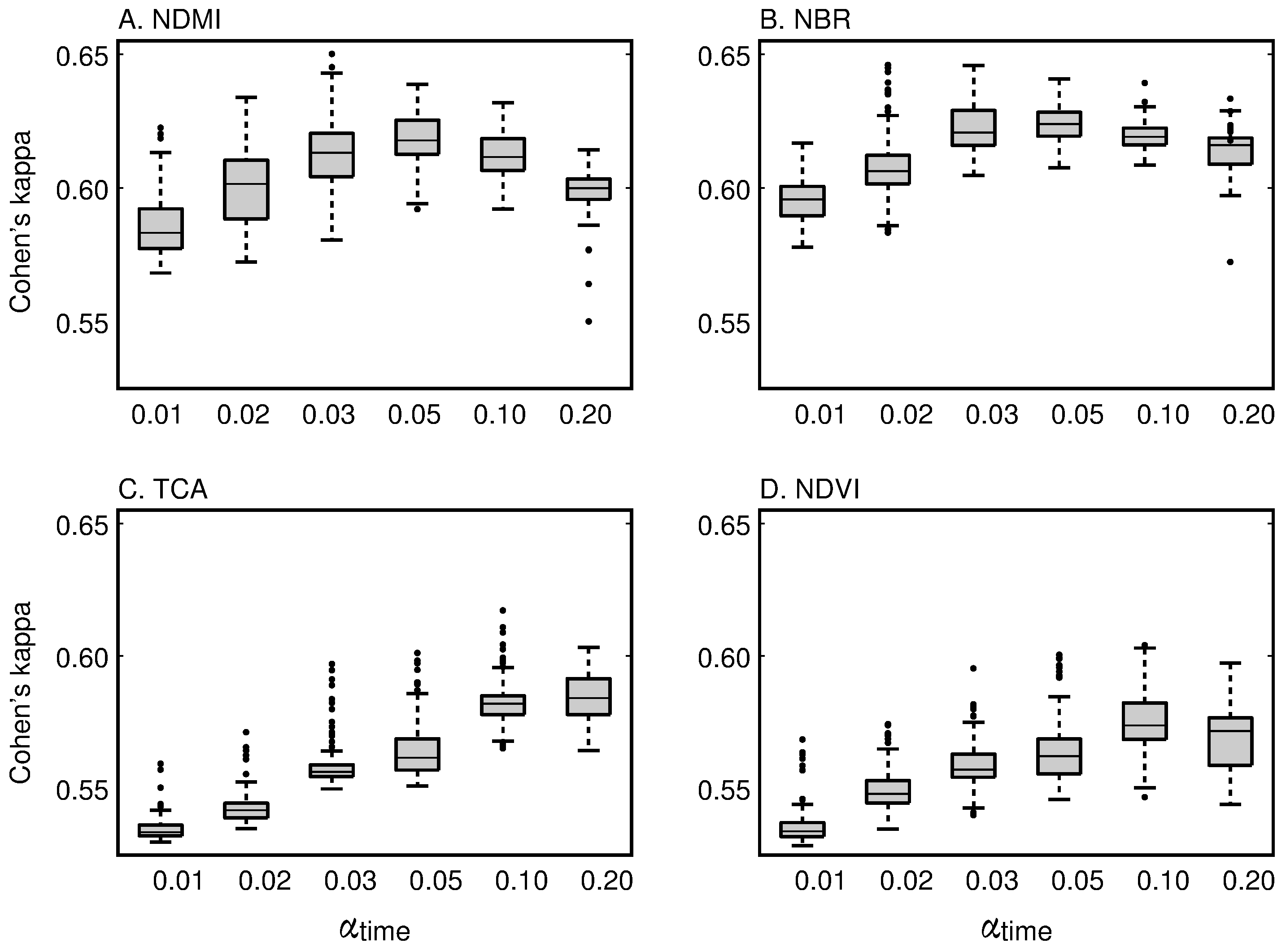
Figure 8.
Distribution of optimal classification thresholds between disturbance and stability (A) and stability and regeneration (B) by amount of simplification applied to the original temporal signal.
Figure 8.
Distribution of optimal classification thresholds between disturbance and stability (A) and stability and regeneration (B) by amount of simplification applied to the original temporal signal.

Figure 9.
Comparison of VeRDET segmentation (solid lines) and labeling (disturbance: orange, stable: blue, regenerating: green) to expert segmentation (vertical dashed lines) with values from summertime composites for two evaluation pixels, a wildfire event showing off-by-one-year errors in disturbance detection (A) and a repeated harvest illustrating disagreement on ‘stability’ versus ‘growth’ after rapid spectral recovery (B).

Figure 10.
Changescape of forests in the Eastern United States over 28 years. Darker areas experience more frequent and intense change than lighter areas, which have primarily stable time series. Red areas experienced primarily disturbance, with dark red areas having sudden intense disturbances and lighter red areas exhibiting stress. Blue areas experienced primarily growth, typically regeneration from a previous disturbance, and green areas experienced a balanced mix of disturbance and regeneration likely due to agriculture or timber management.
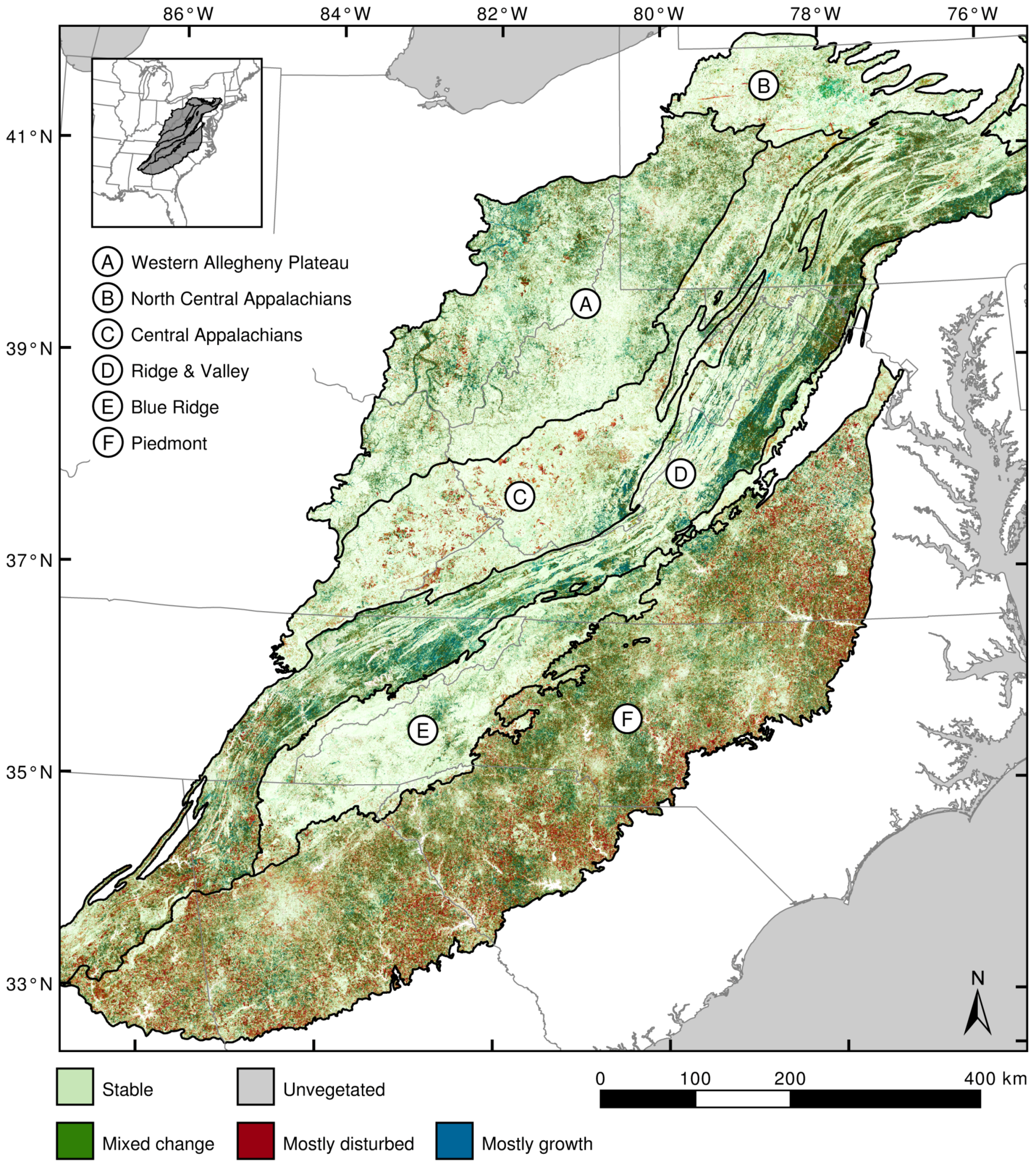
Figure 11.
Percent of forested area experiencing disturbance (solid) and regeneration (dotted) by ecoregion (A–F) over 28 years.
Figure 11.
Percent of forested area experiencing disturbance (solid) and regeneration (dotted) by ecoregion (A–F) over 28 years.
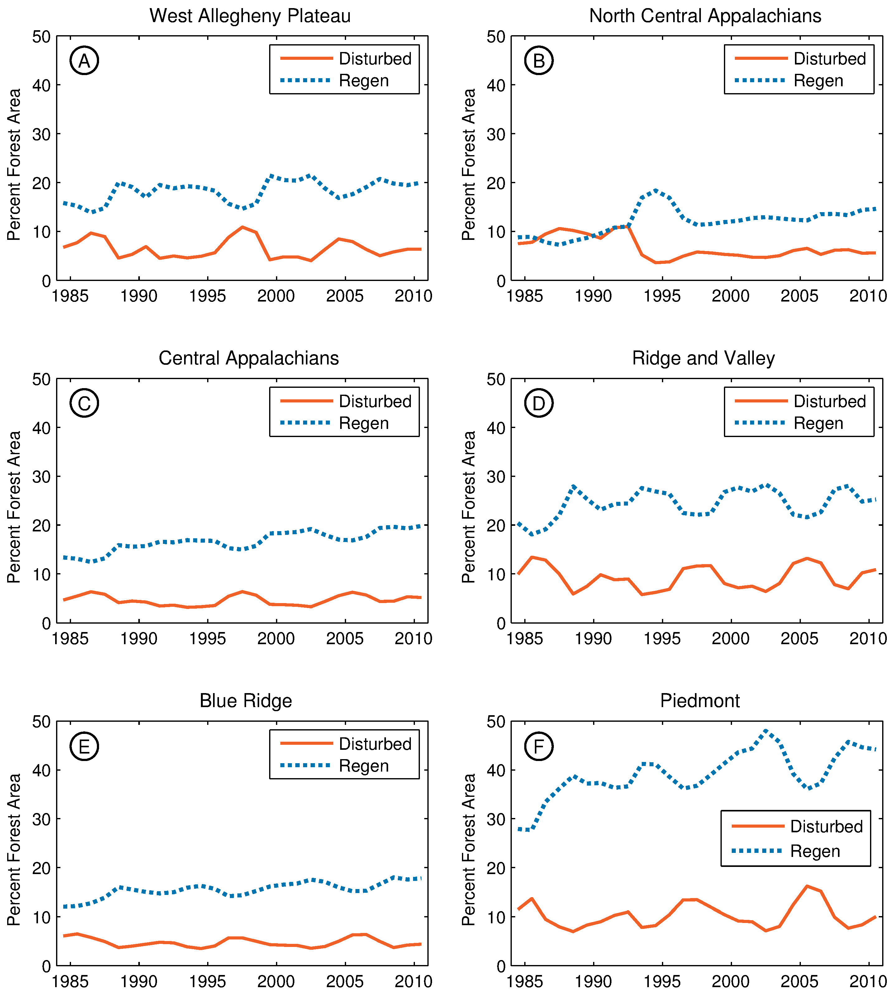
Figure 12.
Detail of a changescape patch exhibiting mixed disturbance. Bark beetles attacked the core of the patch (blue) beginning in 1999, which mostly re-greened by 2005, and then burned along with its surrounding area (red) in a 2009 wildfire.
Figure 12.
Detail of a changescape patch exhibiting mixed disturbance. Bark beetles attacked the core of the patch (blue) beginning in 1999, which mostly re-greened by 2005, and then burned along with its surrounding area (red) in a 2009 wildfire.


Table 1.
Agreement between the VeRDET segmentation and the expert segmentation on whether in each year a sampled location was being disturbed, stable, or regenerated. Experts distinguished between different types of disturbance events.
Table 1.
Agreement between the VeRDET segmentation and the expert segmentation on whether in each year a sampled location was being disturbed, stable, or regenerated. Experts distinguished between different types of disturbance events.
| Expert Label: | Disturbed | Stable | Regen | Commission | |||||
|---|---|---|---|---|---|---|---|---|---|
| Stress | Wind | Wildfire | Mechan. | Harvest | Site Prep. | ||||
| VeRDET Label: | |||||||||
| Disturbed | 6 | 6 | 7 | 69 | 264 | 12 | 617 | 421 | 74.0% |
| Stable | 19 | 5 | 1 | 28 | 95 | 14 | 9425 | 3530 | 28.1% |
| Regen | 2 | 6 | 1 | 12 | 36 | 7 | 1704 | 3996 | 30.7% |
| Omission | 77.8% | 64.7% | 22.2% | 36.7% | 33.2% | 63.6% | 19.8% | 49.7% | 32.0% |
Table 2.
Agreement between the VeRDET segmentation and the expert segmentation after snapping VeRDET breakpoints to expert breakpoints given a 1-year tolerance.
Table 2.
Agreement between the VeRDET segmentation and the expert segmentation after snapping VeRDET breakpoints to expert breakpoints given a 1-year tolerance.
| Expert Label: | Disturbed | Stable | Regen | Commission | |||||
|---|---|---|---|---|---|---|---|---|---|
| Stress | Wind | Wildfire | Mechan. | Harvest | Site Prep. | ||||
| VeRDET Label: | |||||||||
| Disturbed | 7 | 6 | 8 | 73 | 272 | 27 | 450 | 216 | 62.9% |
| Stable | 18 | 5 | 0 | 25 | 90 | 2 | 9722 | 2941 | 24.1% |
| Regen | 2 | 6 | 1 | 11 | 33 | 4 | 1574 | 4790 | 25.4% |
| Omission | 74.1% | 64.7% | 11.1% | 33.0% | 31.1% | 18.2% | 17.2% | 39.7% | 26.5% |
© 2017 by the authors. Licensee MDPI, Basel, Switzerland. This article is an open access article distributed under the terms and conditions of the Creative Commons Attribution (CC BY) license (http://creativecommons.org/licenses/by/4.0/).
Share and Cite
MDPI and ACS Style
Hughes, M.J.; Kaylor, S.D.; Hayes, D.J. Patch-Based Forest Change Detection from Landsat Time Series. Forests 2017, 8, 166. https://doi.org/10.3390/f8050166
AMA Style
Hughes MJ, Kaylor SD, Hayes DJ. Patch-Based Forest Change Detection from Landsat Time Series. Forests. 2017; 8(5):166. https://doi.org/10.3390/f8050166
Chicago/Turabian StyleHughes, M. Joseph, S. Douglas Kaylor, and Daniel J. Hayes. 2017. "Patch-Based Forest Change Detection from Landsat Time Series" Forests 8, no. 5: 166. https://doi.org/10.3390/f8050166
Note that from the first issue of 2016, this journal uses article numbers instead of page numbers. See further details here.