A Linkage among Tree Diameter, Height, Crown Base Height, and Crown Width 4-Variate Distribution and Their Growth Models: A 4-Variate Diffusion Process Approach

Abstract

The evolution of the 4-variate probability distribution of the diameter at the breast height, total height, crown base height, and crown width against the age in a forest stand is of great interest to forest management and the evaluation of forest resources. This paper focuses on the Vasicek type 4-variate fixed effect stochastic differential equation (SDE) to quantify the dynamic of tree size components distribution against the age. The new derived 4-variate probability density function and its marginal univariate, bivariate, trivariate, and conditional univariate distributions are applied for the modeling of stand attributes such as the mean diameter, height, crown base height, crown width, volume, and slenderness. All parameters were estimated by the maximum likelihood procedure using a dataset of 1630 Scots pine trees (12 stands). The results were validated using a dataset of 699 Scots pine trees (five stands). A newly developed 4-variate simultaneous system of SDEs incorporated covariance structure driving changes in tree size components and improved predictions in one tree size component given the other tree size components in the system.

1. Introduction

In forestry literature, different mechanisms have been proposed to describe relationships between components of a tree size in a stand including the diameter at breast height (in the sequel-diameter), total height (in the sequel-height), crown base height, crown width, and age. Traditionally, linear or nonlinear regression relationships were used to relate response components and predictor components [1]. These relationships are useful for estimating the stem volume, crown volume, stand biomass, productivity, and much more. However, for the most part, relationships are deduced at a given tree age (static relationships) and are not sufficient to analyze the long-time evolution of tree size components [2]. Note that the linear or nonlinear regression relationships presented in previous studies provide information about the stem and crown dimensions that can be predicted at a given set of predictor variables; however, they do not relate stem and crown dynamics to the age dimension, and do not consider the underlying covariance structure driving changes in the tree diameter, height, crown base height, and crown width. Unfortunately, the problem of constructing age-diameter regression relationships defies a precise solution as the rate of the stem and crown size components is highly variable. There is another basic issue to keep in mind, in that the growth conditions in a stand regulate links between tree size components and their variations. It seems likely that mathematical techniques to explain covariances of observed tree size components, which arise due to randomness in growth conditions, could be formulated by a probability density function [3].

The most popular static probability density functions used to model diameter distributions are those of the lognormal, gamma, beta, Johnson’s SB, and Weibull functions (e.g., Reference [4] and references therein). Many forms of probability density functions for height distribution such as Weibull, gamma, normal and lognormal, and many more may be chosen [5]. The joint bivariate distribution of tree diameter and height are formulated by Johnson’s SBB, Weibull, Logit-Logistic, or the copula approach (e.g., Reference [6] and references therein).

In the past decades, more and more detailed mathematical distributional models have been developed that faithfully use SDEs and describe the univariate and bivariate evolution of the structure of growth variables in ecology and finance as a more realistic alternative to the classical nonlinear regression models [7,8,9]. The Gompertz, Verhulst, Bertalanffy, and Maltussian type SDEs were used to model the total tree height over age [10] and diameter [11,12], to model the stem taper [13], and to model tree crown width over diameter [14]. They found that the SDE models provided much more accurate predictions of individual tree height and crown width compared to nonlinear regression models. From a practical point of view of forest stand growth modeling, the SDE becomes of great significance as the underlying deterministic mechanisms linking tree size components and age are not fully known. Therefore, the functional relationships between the diameter, height, crown base height, crown width, and age could be mathematically formalized using a 4-variate stochastic process. This study focuses on a new modeling paradigm formulated as a system of 4-variate SDEs which relates basic tree size components (diameter, height, crown base height, and crown width) with the age of a tree.

The basic 4-variate SDE model for the diameter, height, crown base height, and crown width dynamic, where X(t) = (X₁(t), X₂(t), X₃(t), X₄(t))^T = (D(t), H(t), CH(t), CW(t))^T, can be described by:

$$dX\left(t\right)=\mu (X(t),\theta )dt+b(X(t),\theta )dW\left(t\right), P\left(X(t_0)=x_0\right)=1$$

(1)

where $W(t){,}_{}t\ge t_0$ represents standard 4-variate Brownian motion. Intuitively, in this work, the term $dW(\cdot )$ is interpreted as ecological and environmental noise. A parametric approach assumes that the drift $\mu (X(t),\theta )$ (Gompertz, Verhulst, Bertalanffy, gamma, and Maltussian types are special cases of SDEs) and diffusion $b(X(t),\theta )$, representing the model of the covariance structure are known functions with the exception of an unknown fixed-effects parameter vector $\theta$. For special cases of drift and diffusion terms, this SDE asserts that the solution is distributed according to a normal or lognormal distribution with a time dependent mean vector and covariance matrix. The idea is to compute the mean and variance trends for response variables (tree size components) at given predictor variables (tree size components) over time. A newly developed 4-variate SDE model would be superior to the regression models in accordance to the underlying dynamical covariance structure driving changes in the tree size components, and the link among conditional tree size components distribution and mean and variance trends of tree size components.

In the practical context, the fundamental goal of this study is to propose a 4-variate Vasicek type SDEs model, to formalize the corresponding results on statistical inference, and to fit it to a real Scots pine (Pinus Sylvestris L.) tree dataset (diameter, height, crown base height, crown width, and age). All results are implemented in the symbolic algebra system MAPLE.

2. Materials and Methods

2.1. Stochastic Differential Equation Model

One of the important problems in the modeling of a forest stand dynamic is the specification of the multidimensional stochastic process governing the behavior of underlying tree size components. This study supposes that at the age t, the underlying tree size components vector is a random process and denoted by X(t). In the sequel, the tree diameter, tree height, crown base height, and crown width as response variables, X(t) = (X₁(t), X₂(t), X₃(t), X₄(t))^T = (D(t), H(t), CH(t), CW(t))^T, are modeled by a system of 4-variate SDEs against the tree age. In an even-aged stand tree, the size components distribution shows some symmetry (tree size components distribution underlying the dataset tends to the normal distribution), as most trees cluster near the average size with decreasing frequencies at large and small sizes. The Vasicek type SDE is proposed due to its solutions with the normal shape transition probability density function. The Itô [15] system of the Vasicek type SDEs describing the dynamic of the 4-variate random process takes the following form:

$$dX(t)=A\left(X(t)\right)dt+B^{\frac{1}{2}}\cdot dW(t), P\left(X(t_0)=x^0\right)=1,$$

(2)

here: $t\in \left[t_0;T\right]$, $t_0\ge 0$, $X(t_0)=x^0={(x_1^0,x_2^0,x_3^0,x_4^0)}^T$, $W(t)={\left(W_1(t),W_2(t),W_3(t),W_4(t)\right)}^T$ is a 4-variate Brownian motion (“white noise”); ${\alpha }_i,{\beta }_i,\hspace{0.17em}1\le i\le 4$, ${\sigma }_{i,j},\hspace{0.17em}1\le i,j\le 4$ are fixed effect parameters to be estimated; ${\alpha }_i,\hspace{0.17em}1\le i\le 4$ represents asymptotic maximum tree size parameters; ${\beta }_i,\hspace{0.17em}1\le i,j\le 4$ represents the speed of mean reversion at which the process tends to go around the value of ${\alpha }_i,\hspace{0.17em}1\le i\le 4$; ${\sigma }_{i,j},\hspace{0.17em}1\le i,j\le 4$ represents volatility parameters; the drift term $A(x)$ is defined as:

$$A(x)={\left({\beta }_1\left({\alpha }_1-x_1\right),{\beta }_2\left({\alpha }_2-x_2\right),{\beta }_3\left({\alpha }_3-x_3\right),{\beta }_4\left({\alpha }_4-x_4\right)\right)}^T,$$

(3)

and the diffusion term B is defined as:

$$B=\left(\begin{array}{cccc}{\sigma }_{11}& {\sigma }_{12}& {\sigma }_{13}& {\sigma }_{14}\\ {\sigma }_{12}& {\sigma }_{22}& {\sigma }_{23}& {\sigma }_{24}\\ {\sigma }_{13}& {\sigma }_{23}& {\sigma }_{33}& {\sigma }_{34}\\ {\sigma }_{14}& {\sigma }_{24}& {\sigma }_{34}& {\sigma }_{44}\end{array}\right).$$

(4)

The Vasicek type system of the SDEs defined by Equation (2) verifies the conditions of the existence and the uniqueness theorem for SDEs [16]. Therefore, SDE (1) has a unique strong 4-variate solution of $\left(X(t)|X(t_0)=x_0\right)={\left(X_i(t)|X_i(t_0)=x_i^0,\hspace{0.17em}i=1,...,4\right)}^T$, which satisfies the initial condition $P\left(X(t_0)=x^0\right)=1$ and represents a diffusion process with a drift vector defined by Equation (3) and diffusion matrix defined by Equation (4). Using the Itô formula [15], SDE (1) can be converted into a well-studied Ornstein-Uhlenbeck process [17] by transformation $Y(t)={\left(e^{{\beta }_{i}t}{X}_i(t),\hspace{0.17em}i=1,...,4\right)}^T$ in the following form:

$$dY(t)=\underset{\_}{e^{\beta t}}\underset{\_}{\beta \alpha }dt+\underset{\_}{e^{\beta t}}{B}^{\frac{1}{2}}\cdot dW(t), P\left(Y(t_0)=e^{\beta t_0}{x}^0\right)=1,$$

(5)

where we denote: $\underset{\_}{\alpha }={\left({\alpha }_i,\hspace{0.17em}i=1,...,4\right)}^T$, $\underset{\_}{\beta \alpha }={\left({\beta }_i{\alpha }_i,\hspace{0.17em}i=1,...,4\right)}^T$ $\underset{\_}{e^{\beta t}}=\left(\begin{array}{cccc}{e}^{{\beta }_{1}t}& 0& 0& 0\\ 0& e^{{\beta }_{2}t}& 0& 0\\ 0& 0& e^{{\beta }_{3}t}& 0\\ 0& 0& 0& e^{{\beta }_{4}t}\end{array}\right)$.

By integration we have:

$$Y(t)=Y(t_0)+\left(\underset{\_}{e^{\beta t}}-\underset{\_}{e^{\beta t_0}}\right)\underset{\_}{\alpha }+B^{\frac{1}{2}}\cdot {\displaystyle \underset{t_0}{\overset{t}{\int }}\underset{\_}{e^{\beta u}}dW(u)}.$$

(6)

The analytical expression of the process $\left(X(t)|X(t_0)=x_0\right)={\left(X_i(t)|X_i(t_0)=x_i^0,\hspace{0.17em}i=1,...,4\right)}^T$, $t\in \left[t_0;\hspace{0.17em}T\right]$ can be deduced in the following form:

$$X(t)=\underset{\_}{e^{-\beta (t-t_0)}}{x}^0+\left(1-\underset{\_}{e^{-\beta \left(t-t_0\right)}}\right)\underset{\_}{\alpha }+\underset{\_}{e^{\beta t}}{B}^{\frac{1}{2}}\cdot {\displaystyle \underset{t_0}{\overset{t}{\int }}\underset{\_}{e^{\beta u}}dW(u)}.$$

(7)

Taking into account that the last term in Equation (6) has a 4-variate normal distribution, we can deduce that the conditional random vector $\left(X(t)|X(t_0)=x_0\right)={\left(X_i(t)|X_i(t_0)=x_i^0,\hspace{0.17em}i=1,...,4\right)}^T$ has a 4-variate normal distribution of $N_4\left(\mu (t);\hspace{0.17em}\Sigma (t)\right)$, with the mean vector $\mu (t)={\left({\mu }_i(t),\hspace{0.17em}i=1,...,4\right)}^T$ defined by:

$$\mu (t)=\underset{\_}{e^{-\beta (t-t_0)}}{x}^0+\left(1-\underset{\_}{e^{-\beta \left(t-t_0\right)}}\right)\underset{\_}{\alpha }={\left({\alpha }_i+\left(x_i^0-a_i\right)e^{-{\beta }_i\left(t-t_0\right)},\hspace{0.17em}i=1,...,4\right)}^T,$$

(8)

the variance-covariance matrix $\Sigma (t)$:

$$\Sigma (t)={\displaystyle \underset{t_0}{\overset{t}{\int }}\underset{\_}{e^{\beta (u-t)}}B\underset{\_}{e^{\beta (u-t)}}}du={\left(\frac{{\sigma }_{ij}}{{\beta }_i+{\beta }_j}\left(1-e^{-({\beta }_i+{\beta }_j)(t-t_0)}\right)\right)}_{i,j=1,...,4},$$

(9)

and probability density function:

$$f\left(x_1,x_2,x_3,x_4,t|\theta \right)=\frac{1}{{\left(2\pi \right)}^2{\left|\Sigma (t)\right|}^{\frac{1}{2}}}\exp \left(-\frac{1}{2}\Omega (x_1,x_2,x_3,x_4,t)\right).$$

(10)

$$\Omega (x_1,x_2,x_3,x_4,t)={\left(x-\mu (t)\right)}^T{\left(\Sigma (t)\right)}^{-1}\left(x-\mu (t)\right)$$

(11)

$$\theta =\left\{{\alpha }_1,{\beta }_1,\hspace{0.17em}{\alpha }_2,{\beta }_2,{\alpha }_3,{\beta }_3,{\alpha }_4,{\beta }_4,\hspace{0.17em}{\sigma }_{11},\hspace{0.17em}{\sigma }_{12},{\sigma }_{13},\hspace{0.17em}{\sigma }_{22},{\sigma }_{23},{\sigma }_{24},{\sigma }_{33},{\sigma }_{34}\right\}$$

(12)

2.2. Marginal and Conditional Distributions

Allowing that the random vector $\left(X(t)|X(t_0)=x_0\right)={\left(X_i(t)|X_i(t_0)=x_i^0,\hspace{0.17em}i=1,...,4\right)}^T$ has a 4-variate normal distribution of $N_4\left(\mu (t);\hspace{0.17em}\Sigma (t)\right)$ defined by Equations (8)–(10) and refers to properties of multivariate normal distribution [18], the marginal univariate distribution of $\left(X_i(t)|X_i(t_0)=x_i^0\right)$, $1\le i\le 4$ is also normal $N_1\left({\mu }_i(t);\hspace{0.17em}{v}_{i,i}^2(t)\right)$, and $1\le i\le 4$ with mean and variance functions given by the following forms and probability density function:

$${\mu }_i(t)={\rm E}\left(X_i(t)|X_i(t_0)=x_i^0\right)={\alpha }_i+\left(x_i^0-a_i\right)e^{-{\beta }_i\left(t-t_0\right)},$$

(13)

$$v_{i,i}^2(t)=Var\left(X_i(t)|X_i(t_0)=x_i^0\right)=\frac{{\sigma }_{ii}}{2{\beta }_i}\left(1-e^{-2{\beta }_i(t-t_0)}\right).$$

(14)

The marginal bivariate distribution of $\left(X_j(t)|X_j(t_0)=x_j^0,\hspace{0.17em}{X}_k(t)|X_k(t_0)=x_k^0\right)$, $1\le j,k\le 4$, is normal $N_2\left({\mu }^2(t);\hspace{0.17em}{\Sigma }_{22}(t)\right)$, with the mean vector ${\mu }^2(t)={\left({\mu }_j(t),\hspace{0.17em}{\mu }_k(t)\right)}^T$ defined by:

$${\mu }^2(t)={\left({\alpha }_j+\left(x_j^0-a_j\right)e^{-{\beta }_j\left(t-t_0\right)},\hspace{0.17em}{\alpha }_k+\left(x_k^0-a_k\right)e^{-{\beta }_k\left(t-t_0\right)}\right)}^T,$$

(15)

the variance-covariance matrix ${\Sigma }_{22}(t)$ given by:

$${\Sigma }_{22}(t)=\left(\begin{array}{cc}{v}_{j,j}^2(t)& v_{j,k}^2(t)\\ v_{k,j}^2(t)& v_{k,k}^2(t)\end{array}\right),$$

(16)

and the coefficient of correlation defined by:

$${\rho }_{j,k}(t)=\frac{v_{j,k}^2(t)}{\sqrt{v_{j,j}^2(t)\cdot v_{k,k}^2(t)}}.$$

(17)

The marginal trivariate distribution of $\left(X_j(t)|X_j(t_0)=x_j^0,\hspace{0.17em}{X}_k(t)|X_k(t_0)=x_k^0,\hspace{0.17em}{X}_l(t)|X_l(t_0)=x_l^0\right)$, $1\le j,k,l\le 4$, is normal with the mean vector ${\mu }^3(t)={\left({\mu }_j(t),\hspace{0.17em}{\mu }_k(t),\hspace{0.17em}{\mu }_l(t)\right)}^T$ and the variance-covariance matrix ${\Sigma }_{33}(t)$ defined by:

$${\mu }^3(t)={\left({\alpha }_j+\left(x_j^0-a_j\right)e^{-{\beta }_j\left(t-t_0\right)},\hspace{0.17em}{\alpha }_k+\left(x_k^0-a_k\right)e^{-{\beta }_k\left(t-t_0\right)},\hspace{0.17em}{\alpha }_l+\left(x_l^0-a_l\right)e^{-{\beta }_l\left(t-t_0\right)}\right)}^T,$$

(18)

$${\Sigma }_{33}(t)=\left(\begin{array}{ccc}{v}_{j,j}^2(t)& v_{j,k}^2(t)& v_{j,l}^2(t)\\ v_{k,j}^2(t)& v_{k,k}^2(t)& v_{k,l}^2(t)\\ v_{l,j}^2(t)& v_{l,k}^2(t)& v_{l,l}^2(t)\end{array}\right).$$

(19)

The conditional distribution of $\left(X_i(t)|X_i(t_0)=x_i^0\right)$, $1\le i\le 4$, at a given $\left(X_j(t)=x_j,\text{}\hspace{0.17em}{X}_k(t)=x_k,\hspace{0.17em}{X}_l(t)=x_l\right)$, $j,k,l\in \left\{1,2,3,4\right\}\backslash \left\{i\right\}$, is a univariate normal $N_1\left({\eta }_i^3(t,x_j,x_k,x_l);\hspace{0.17em}{\lambda }_{i,3}^2(t)\right)$. Using Equations (18) and (19), the mean and variance can be computed in the following form:

$${\eta }_i^3\left(t,x_j,x_k,x_l\right)={\rm E}\left(X_i(t)|X_j(t)=x_j,\text{}\hspace{0.17em}{X}_k(t)=x_k,\hspace{0.17em}{X}_l(t)=x_l\right)={\mu }_i(t)+{\Sigma }_{13}(t){\left[{\Sigma }_{33}(t)\right]}^{-1}{\mu }^3(t),$$

(20)

$${\lambda }_{i,3}^2\left(t\right)=Var\left(X_i(t)|X_j(t)=x_j,\text{}\hspace{0.17em}{X}_k(t)=x_k,\hspace{0.17em}{X}_l(t)=x_l\right)=v_{ii}^2(t)-{\Sigma }_{13}(t){\left[{\Sigma }_{33}(t)\right]}^{-1}{\left({\Sigma }_{13}(t)\right)}^T,$$

(21)

where ${\Sigma }_{13}(t)=\left(\begin{array}{ccc}{v}_{i,j}^2(t)& v_{i,k}^2(t)& v_{i,l}^2(t)\end{array}\right)$.

The conditional distribution of $\left(X_i(t)|X_i(t_0)=x_i^0\right)$, $1\le i\le 4$ at a given $\left(X_j(t)=x_j,\text{}\hspace{0.17em}{X}_k(t)=x_k\right)$, $j,k\in \left\{1,2,3,4\right\}\backslash \left\{i\right\}$, is a univariate normal $N_1\left({\eta }_i^2(t,x_j,x_k);\hspace{0.17em}{\lambda }_{i,2}^2(t)\right)$. Using Equations (15) and (16), the mean and variance can be computed in the following form:

$${\eta }_i^2\left(t,x_j,x_k\right)={\rm E}\left(X_i(t)|X_j(t)=x_j,\text{}\hspace{0.17em}{X}_k(t)=x_k\right)={\mu }_i(t)+{\Sigma }_{12}(t){\left[{\Sigma }_{22}(t)\right]}^{-1}{\mu }^3(t),$$

(22)

$${\lambda }_{i,2}^2\left(t\right)=Var\left(X_i(t)|X_j(t)=x_j,\text{}\hspace{0.17em}{X}_k(t)=x_k\right)=v_{ii}^2(t)-{\Sigma }_{12}(t){\left[{\Sigma }_{22}(t)\right]}^{-1}{\left({\Sigma }_{12}(t)\right)}^T,$$

(23)

where ${\Sigma }_{12}(t)=\left(\begin{array}{cc}{v}_{i,j}^2(t)& v_{i,k}^2(t)\end{array}\right)$.

The conditional distribution of $\left(X_i(t)|X_i(t_0)=x_i^0\right)$, $1\le i\le 4$, at a given $\left(X_j(t)=x_j\right)$, $j\in \left\{1,2,3,4\right\}\backslash \left\{i\right\}$, is a univariate normal $N_1\left({\eta }_i^1(t,x_j);\hspace{0.17em}{\lambda }_{i,1}^2(t)\right)$. Using Equations (15)–(17), the mean and variance can be computed in the following form:

$${\eta }_i^1\left(t,x_j\right)={\rm E}\left(X_i(t)|X_j(t)=x_j\right)={\mu }_i(t)+\frac{v_{i,j}^2(t)}{v_{j,j}^2(t)}\left(x_j-{\mu }_j(t)\right),$$

(24)

$${\lambda }_{i,1}^2\left(t\right)=Var\left(X_i(t)|X_j(t)=x_j\right)=\left(1-{\rho }^2(t)\right)v_{ii}^2(t).$$

(25)

In summary, Equations (21), (23), and (25) show us that the univariate conditional distributions of the ith tree size component (diameter, height, crown height, and crown width) exhibit an age dependent variance which is the same for each prior listed scenarios of predictor tree size components.

2.3. Maximum Likelihood Estimates

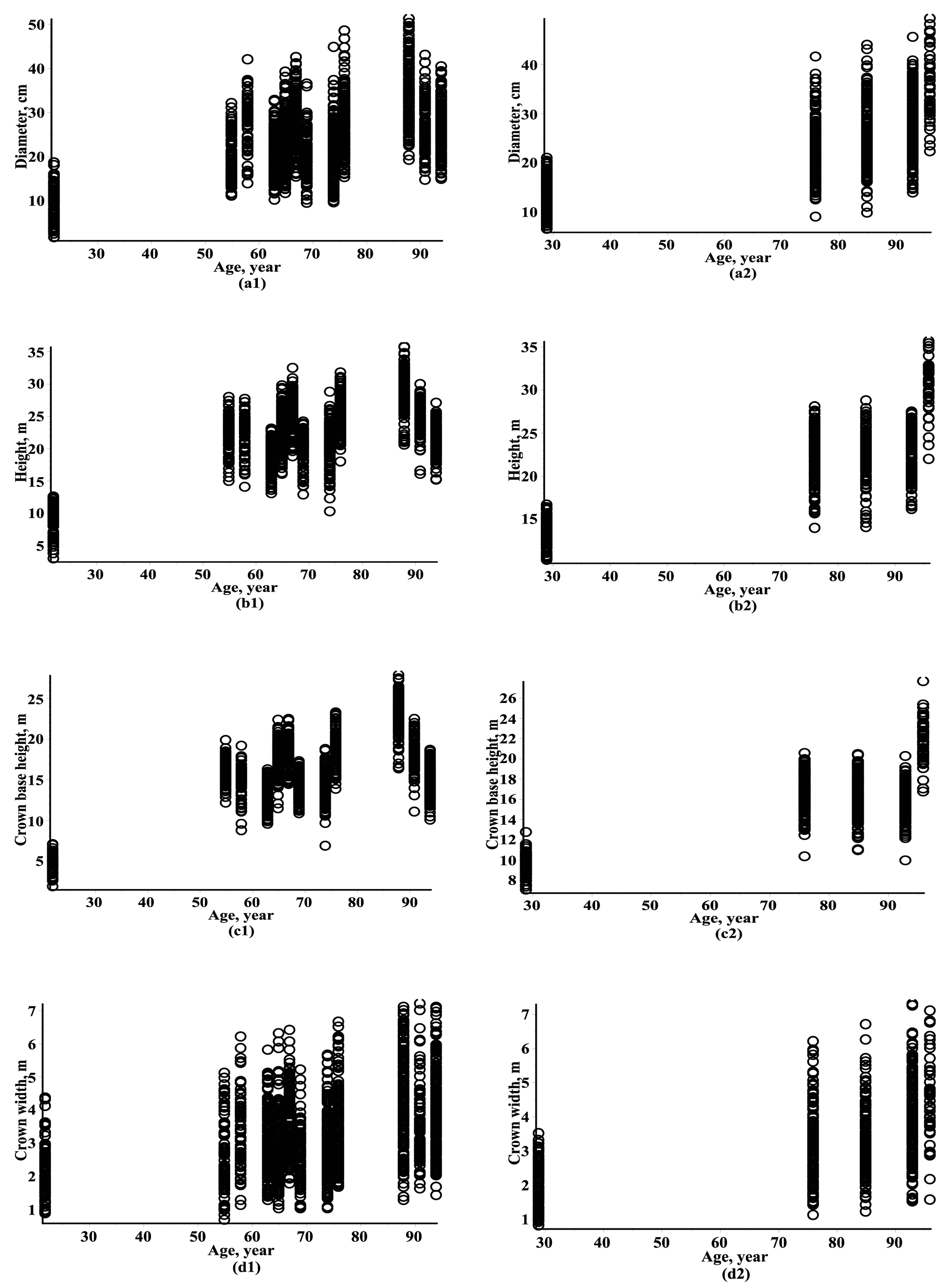
The SDE model defined by Equation (2) can be fitted to diameter (x₁), height (x₂), crown base height (x₃), and crown width (x₄) samples $\left\{\left(x_{1,1}^i,x_{2,1}^i,x_{3,1}^i,x_{4,1}^i\right),\hspace{0.17em}\left(x_{1,2}^i,x_{2,2}^i,x_{3,2}^i,x_{4,2}^i\right),\hspace{0.17em}\hspace{0.17em}\dots ,\hspace{0.17em}\left(x_{1,n_i}^i,x_{2,n_i}^i,x_{3,n_i}^i,x_{4,n_i}^i\right)\right\}$ at discrete times (ages) $\left\{t_1^i,\hspace{0.17em}{t}_2^i,\hspace{0.17em}\hspace{0.17em}\dots ,\hspace{0.17em}{t}_{n_i}^i\right\}$ (n_i is the number of observed trees of the ith plot, $i=1,\hspace{0.17em}2,\hspace{0.17em}...,\hspace{0.17em}M$) by the maximum likelihood procedure. The associated maximum likelihood function for the 4-variate fixed effect SDE model takes the following form:

$$L(\theta )={\displaystyle \prod _{i=1}^M{\displaystyle \prod _{j=1}^{n_i}f\left(x_{1,j}^i,x_{2,j}^i,x_{3,j}^i,x_{4,j}^i,t_j^i|\theta \right)}},$$

(26)

and the maximum log-likelihood function is:

$$LL(\theta )={\displaystyle \sum _{i=1}^M{\displaystyle \sum _{j=1}^{n_i}\ln \left(f\left(x_{1,j}^i,x_{2,j}^i,x_{3,j}^i,x_{4,j}^i,t_j^i|\theta \right)\right)}},$$

(27)

where the probability density function $f\left(x_1,x_2,x_3,x_4,t|\theta \right)$ takes the form defined by Equation (10).

2.4. Data

This paper illustrates the new developed modeling technique by using a Scots pine (Pinus Sylvestris L.) tree dataset. All data were collected during 1979–2012 across the entire Lithuanian territory (latitude, 53°54′–56°27′ N; longitude, 20°56′–26°51′ E; altitude, 10–293 m). Mean temperatures vary from −16.4 °C in winter to +22 °C in summer. Precipitation is distributed throughout the year, although predominantly in summer, and the average is approximately 680 mm a year. At plot establishment, the following data were recorded for every sample tree: diameter over bark at 1.30 m; height; crown base height, which was measured as the height of the lowest live branch of a tree; crown width; and age. A total of 17 plots (2329 trees) of the Scots pine trees dataset were compiled at the Aleksandras Stulginskis university. The dataset was randomly divided into estimation and validation datasets. A random sample of 12 plots (1630 trees) was selected for model estimation, and the remaining dataset of five plots (699 trees) was used for model validation. The observed datasets of the diameter, height, crown base height, and crown width measurements are presented in Figure 1.

3. Results and Discussion

3.1. Estimating Results

A good estimate of the fixed effect parameters vector $\theta =\left\{{\alpha }_1,{\beta }_1,\hspace{0.17em}{\alpha }_2,{\beta }_2,{\alpha }_3,{\beta }_3,{\alpha }_4,{\beta }_4,\hspace{0.17em}{\sigma }_{11},\hspace{0.17em}{\sigma }_{12},{\sigma }_{13},\hspace{0.17em}{\sigma }_{22},{\sigma }_{23},{\sigma }_{24},{\sigma }_{33},{\sigma }_{34}\right\}$ of the 4-variate probability density function defined by Equation (10) would be the vector $\stackrel{\wedge }{\theta }$ that maximizes the likelihood of getting the diameter, height, crown base height, and crown width datasets $\left\{\left(x_{1,1}^i,x_{2,1}^i,x_{3,1}^i,x_{4,1}^i\right),\hspace{0.17em}\left(x_{1,2}^i,x_{2,2}^i,x_{3,2}^i,x_{4,2}^i\right),\hspace{0.17em}\hspace{0.17em}\dots ,\hspace{0.17em}\left(x_{1,n_i}^i,x_{2,n_i}^i,x_{3,n_i}^i,x_{4,n_i}^i\right)\right\}$ at discrete times (ages) $\left(t_1^i,t_2^i,\dots ,t_{n_i}^i\right)$. The parameter estimators were calculated by maximization of the log-likelihood function defined by Equation (27) using the NLPSolve procedure in MAPLE [19]. The results of the parameter estimates are summarized in

Table 1. Estimates of parameters.

Parameters of Drift Term
α1	β1	α2	β2	α3	β3	α4	β4
37.3302	0.0174	27.6250	0.0277	24.0573	0.0177	4.9822	0.0137
Parameters of Diffusion Term
σ11	σ12	σ13	σ14	σ22	σ23	σ24	σ33	σ34	σ44
1.8334	1.0057	0.4150	0.2242	0.9010	0.5159	0.0913	0.3937	0.0176	0.0441

.

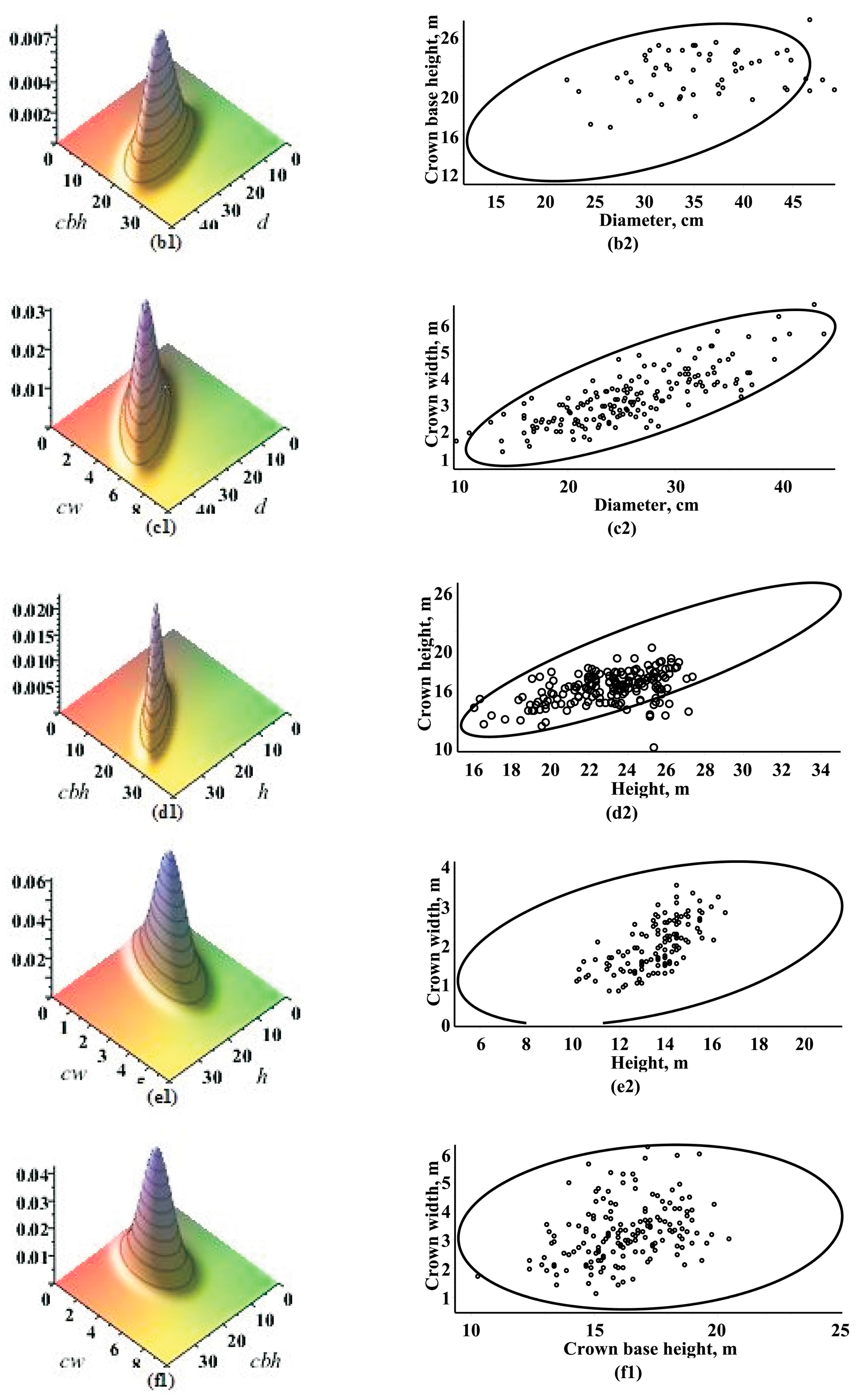
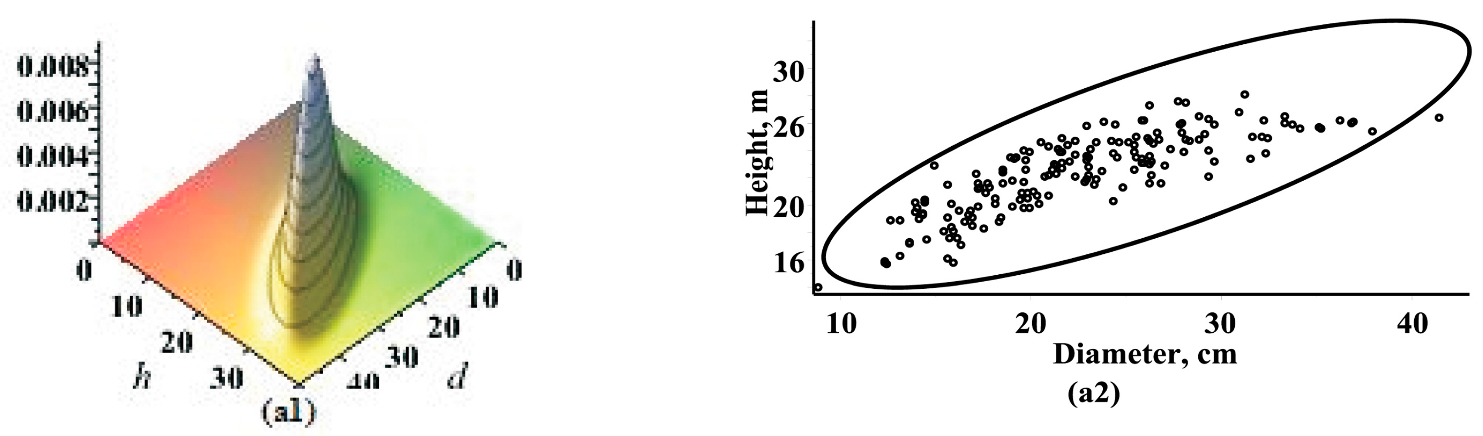
3.2. Marginal Bivariate Distributions

The newly developed 4-variate probability density function defined by Equation (10) is attractive for its multiplicity of cases such as the marginal univariate, bivariate, and trivariate, and conditional univariate, bivariate, and trivariate probability density functions of the tree size components and may be justified from an application perspective.

To demonstrate that the validation dataset of Scots pine trees do indeed follow the marginal bivariate estimated probability density function with the mean vector defined by Equation (15) and the covariance matrix defined by Equation (16), we will use simple graphical techniques. The estimates of parameters $\stackrel{\wedge }{\theta }$ were calculated by the maximum likelihood procedure (see Table 1) using the estimation dataset (see Figure 1). Figure 2 shows the estimated bivariate marginal probability density functions and their 95% confidence regions for all scenarios of tree size components. The bivariate analog of the confidence interval is given by an ellipsoid:

$${\left(x-{\mu }^2(t)\right)}^T{\left[{\Sigma }_{22}(t)\right]}^{-1}\left(x-{\mu }^2(t)\right)={\chi }_2^2(\alpha ),$$

(28)

where vector ${\mu }^2(t)$ and matrix ${\Sigma }_{22}(t)$ are defined by Equations (15) and (16), respectively, $x={\left(x_j,\hspace{0.17em}{x}_k\right)}^T$, $1\le j,k\le 4$, ${\chi }_2^2(\alpha )$ is from the Chi-square distribution with two degrees of freedom. Specifically, if $\alpha =0.05$(${\chi }_2^2(0.05)=5.99$), Equation (28) provides the confidence region containing 95% of the probability mass of the marginal bivariate distribution.

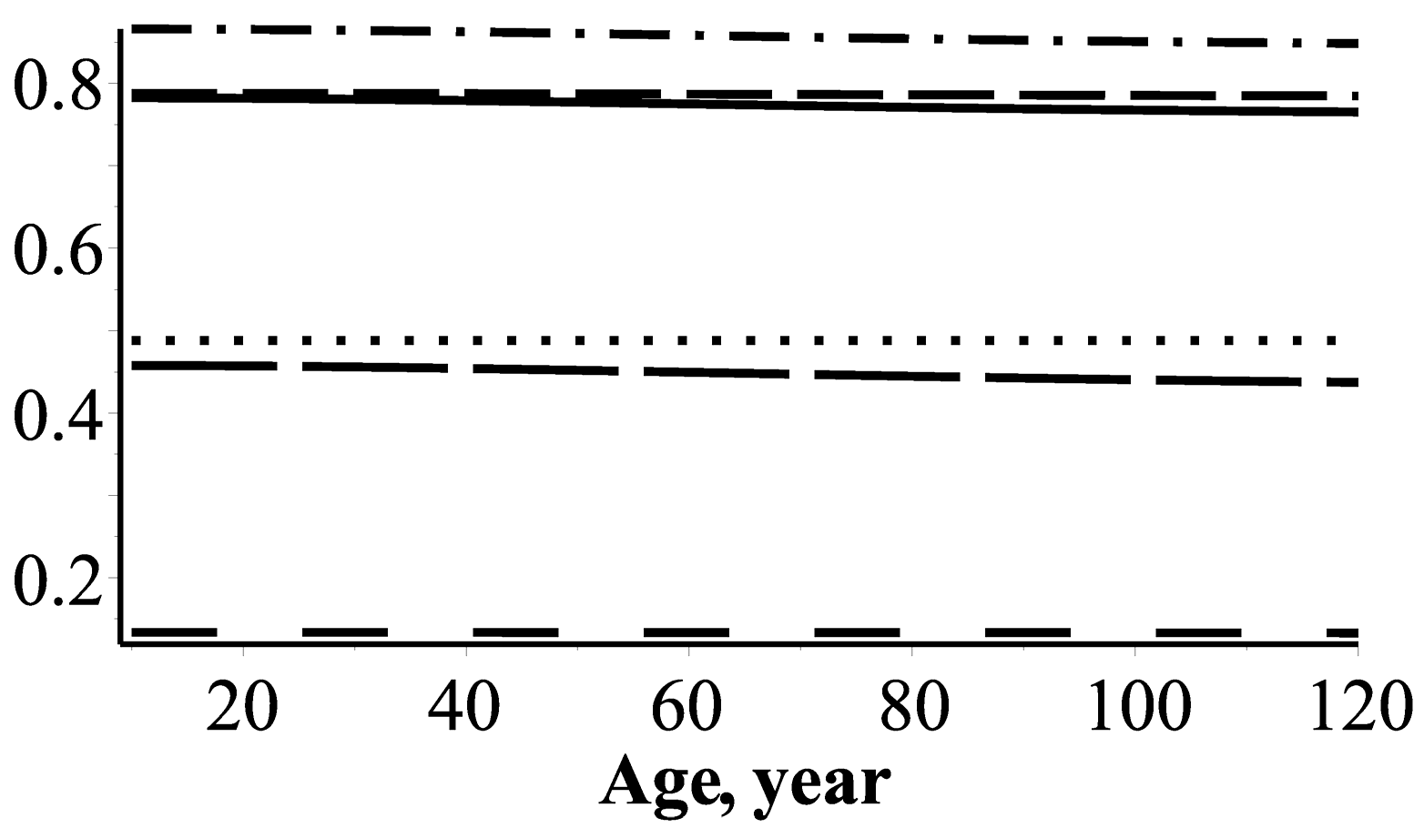
3.3. Coefficient of Correlation

The estimated correlation functions (ECFs) for all scenarios of marginal bivariate distributions are presented in Figure 3. The ECFs play a major role in modeling the dependence among tree size components. It appears from Figure 3 that the highest ECF provided tree height and crown base height, and the lowest ECF provided tree crown base height and crown width.

3.4. Diameter, Height, Crown Base Height and Crown Width Dynamical Models

The evolution of the diameter, height, crown base height, and crown width can be formulated using the marginal univariate probability density function defined by Equations (13) and (14) or the conditional univariate probability density function defined by Equations (20)–(25). The modeling of the diameter, height, crown base height, and crown width was divided into four scenarios:

• in the first scenario, a tree size component was linked to tree age (one model, marginal univariate densities are defined by Equations (13) and (14));
• in the second scenario, a tree size component was linked to tree age and one size component (three models, conditional univariate densities are defined by Equations (24) and (25));
• in the third scenario, a tree size component was linked to tree age and two size components (three models, conditional univariate densities are defined by Equations (22) and (23));
• in the fourth scenario, a tree size component was linked to tree age and three size components (one model, conditional univariate densities are defined by Equations (20) and (21)).

The results concerning the fitting and validating of all the diameter, height, crown base height and crown width dynamical models defined by marginal univariate and conditional univariate probability density functions are presented in

Table 2. Statistical indexes for all models applied to the estimation and validation datasets.

	Estimation				Validation
	B, m (PB, %)	Model	AE, m (Rank)	R2 (Rank)	B, m (PB, %)	AB, m (PAB, %)	AE, m	R2
Diameter
Equation (13) A	−0.006 (−9.079)	5.452 (26.148)	6.800 (8)	0.334 (8)	−0.842 (−10.942)	5.293 (25.612)	6.554 (8)	0.432 (8)
Equation (24) A, H	0.006 (−2.262)	3.409 (15.243)	4.302 (5)	0.733 (5)	0.382 (−1.976)	3.260 (14.354)	4.111 (4)	0.773 (4)
Equation (24) A, CH	0.004 (−5.865)	4.751 (22.162)	5.869 (7)	0.503 (7)	0.376 (−5.605)	4.788 (22.256)	5.990 (7)	0.517 (7)
Equation (24) A, CW	−0.006 (−4.211)	3.237 (15.053)	4.216 (4)	0.744 (4)	−0.491 (−4.368)	3.282 (15.189)	4.186 (5)	0.766 (5)
Equation (22) A, H, CH	0.00001 (−5.377)	4.408 (20.330)	5.452 (6)	0.571 (6)	0.311 (−5.098)	4.441 (20.495)	5.536 (6)	0.587 (6)
Equation (22) A, H, CW	0.002 (−1.021)	2.072 (9.083)	2.731 (2)	0.892 (2)	0.237 (−0.231)	2.240 (9.887)	2.873 (2)	0.889 (2)
Equation (22) A, CH, CW	0.002 (−1.964)	2.479 (11.002)	3.285 (3)	0.844 (3)	0.461 (−0.531)	2.784 (12.370)	3.601 (3)	0.826 (3)
Equation (20) A, H, CH, CW	0.001 (−0.971)	2.034 (9.005)	2.674 (1)	0.896 (1)	0.091 (−0.326)	2.204 (9.964)	2.804 (1)	0.892 (1)
Height
Equation (13) A	−0.016 (−4.085)	3.225 (15.770)	3.926 (8)	0.473 (8)	−0.904 (−5.834)	2.478 (12.032)	3.328 (8)	0.592 (8)
Equation (24) A, D	−0.013 (−2.078)	2.014 (9.818)	2.491 (6)	0.788 (6)	−0.539 (−2.950)	1.654 (7.638)	2.086 (5)	0.837 (5)
Equation (24) A, CH	0.005 (−0.720)	1.603 (7.921)	1.999 (4)	0.863 (4)	0.287 (−0.143)	1.664 (7.977)	2.178 (6)	0.813 (6)
Equation (24) A, CW	−0.019 (−3.661)	2.872 (14.161)	3.510 (7)	0.578 (7)	−0.786 (−4.669)	2.192 (10.382)	2.899 (7)	0.688 (7)
Equation (22) A, D, CH	0.001 (−0.405)	0.968 (4.618)	1.253 (2)	0.946 (1−2)	0.191 (0.085)	1.036 (4.962)	1.320 (2)	0.931 (1)
Equation (22) A, D, CW	−0.009 (−1.623)	1.809 (8.672)	2.276 (5)	0.822 (5)	−0.492 (−2.801)	1.612 (7.501)	2.049 (4)	0841 (4)
Equation (22) A, CH, CW	0.002 (−0.578)	1.200 (5.732)	1.540 (3)	0.919 (3)	0.314 (0.445)	1.291 (6.100)	1.695 (3)	0.888 (3)
Equation (20) A, D, CH, CW	0.001 (−0.406)	0.967 (4.616)	1.252 (1)	0.946 (1–2)	0.074 (1.319)	1.034 (4.956)	1.319 (1)	0.931 (2)
Crown Base Height
Equation (13) A	−0.009 (−5.573)	2.592 (18.191)	3.134 (8)	0.507 (8)	−1.135 (−7.942)	2.148 (14.535)	2.683 (8)	0.554 (8)
Equation (24) A, D	−0.008 (−4.718)	(2.206 (15.889)	2.706 (6)	0.632 (6)	−0.946 (−6.447)	1.914 (12.884)	2.478 (6)	0.602 (6)
Equation (24) A, H	−0.003 (−1.866)	1.272 (9.134)	1.586 (4)	0874 (4)	−0.512 (−2.919)	1.275 (8.714)	1.729 (4)	0.793 (4)
Equation (24) A, CW	−0.009 (−5.649)	2.559 (18.170)	3.079 (7)	0.518 (7)	−1.108 (−7.710)	2.115 (14.330)	2.670 (7)	0.554 (7)
Equation (22) A, D, H	−0.002 (−1.120)	1.060 (7.343)	1.362 (3)	0.907 (3)	−0.439 (−2.294)	1.151 (7.925)	1.500 (2)	0.844 (3)
Equation (22) A, D, CW	−0.006 (−3.432)	1.917 (13.256)	2.414 (5)	0.707 (5)	−0.882 (−6.019)	1.810 (12.061)	2.362 (5)	0.636 (5)
Equation (22) A, H, CW	−0.002 (−1.048)	1.056 (7.159)	1.358 (2)	0.907 (2)	−0.477 (−2.672)	1.130 (7.692)	1.510 (3)	0.844 (2)
Equation (20) A, D, H, CW	−0.001 (−0.989)	1.033 (7.027)	1.329 (1)	0.911 (1)	−0.451 (−2.417)	1.121 (7.585)	1.470 (1)	0.850 (1)
Crown Width
Equation (13) A	−0.0003 (−13.536)	0.908 (33.124)	1.129 (8)	0.141 (8)	−0.066 (−13.737)	0.829 (30.005)	1.048 (8)	0.284 (7)
Equation (24) A, D	0.003 (−4.829)	0.540 (18.554)	0.701 (4)	0.668 (4)	0.047 (−3.294)	0.520 (17.404)	0.671 (4)	0.705 (4)
Equation (24) A, H	0.001 (−10.287)	0.804 (28.622)	1.008 (6)	0.313 (6)	0.054 (−7.652)	0.711 (24.248)	0.918 (6)	0.447 (6)
Equation (24) A, CH	5.7 × 10−6 (−13.161)	0.898 (32.724)	1.115 (7)	0.160 (7)	−0.009 (−12.018)	0.816 (29.099)	1.043 (7)	0.284 (8)
Equation (22) A, D, H	−1.5 × 10−5 (−4.311)	0.4878 (16.699)	0.6410 (3)	0.7214 (3)	0.0163 (−4.661)	0.497 (17.033)	0.645 (3)	0.724 (3)
Equation (22) A, D, CH	−0.0002 (−3.980)	0.474 (16.011)	0.626 (2)	0.734 (1−2)	−0.069 (−5.416)	0.485 (16.477)	0.631 (2)	0.739 (1)
Equation (22) A, H, CH	2.3 × 10−5 (−7.117)	0.670 (22.835)	0.865 (5)	0.492 (5)	−0.111 (−8.290)	0.640 (21.929)	0.805 (5)	0.578 (5)
Equation (20) A, D, H, CH	−0.0001 (−3.977)	0.474 (16.010)	0.6254 (1)	0.734 (1–2)	−0.065 (−5.291)	0.484 (16.446)	0.631 (1)	0.738 (2)

.

The mean prediction bias ($B=\frac{1}{n}{\displaystyle \sum _{i=1}^n\left(y_i-\stackrel{\wedge }{y_i}\right)}$) and the percentage mean prediction bias ($PB=\frac{1}{n}{\displaystyle \sum _{i=1}^n\frac{y_i-\stackrel{\wedge }{y_i}}{y_i}}\cdot 100$), the absolute mean prediction bias ($AB=\frac{1}{n}{\displaystyle \sum _{i=1}^n\left|y_i-\stackrel{\wedge }{y_i}\right|}$) and the percentage mean absolute prediction bias ($AB=\frac{1}{n}{\displaystyle \sum _{i=1}^n\left|\frac{y_i-\stackrel{\wedge }{y_i}}{y_i}\right|}$), an adjusted root mean square error ($AE=\sqrt{B^2+\frac{1}{n-1}{\displaystyle \sum _{i=1}^n{\left(y_i-\stackrel{\wedge }{y_i}-B\right)}^2}}$) and an adjusted coefficient of determination ($R^2=1-\frac{n-1}{n-p}\frac{{\displaystyle \sum _{i=1}^n{\left(y_i-\stackrel{\wedge }{y_i}\right)}^2}}{{\displaystyle \sum _{i=1}^n{\left(y_i-\overline{y}\right)}^2}}$).

Table 2 shows the predictive ability for all newly developed fixed effect parameters diameter, height, crown base height, and crown width growth models for both estimation and validation datasets using the estimates of parameters $\stackrel{\wedge }{\theta }$ presented in Table 1. The models of tree size component evolution show similar statistical indexes for both estimation and validation datasets. The relative importance of the tree size components as predictor variables in all models can be viewed from a goodness of fit standpoint in Table 2. Table 2 shows that the three component scenario models are the largest contribution models. The statistical indexes presented in Table 2 show a low prediction ability for the first scenario models. In the modeling of the tree diameter, the largest contribution arises from the tree height (the second scenario) and from the tree height and crown width (the third scenario). In the modeling of the tree height, the largest contribution arises from the tree diameter (the second scenario) and from the tree diameter and crown base height (the third scenario). In the modeling of the tree crown base height, the largest contribution arises from the tree height (the second scenario) and from the tree height and crown width (the third scenario). In the modeling of the tree crown width, the largest contribution arises from the tree diameter (the second scenario) and from the tree diameter and crown base height (the third scenario).

3.5. Slenderness

The slenderness coefficient is an important characteristic for indexing tree resistance to wind throw and snow damage [20]. The evolution of the tree crown structure is affected by random processes that govern crown movements [21]. In this study, the evolution of the slenderness ratio of the stem and crown, and the crown ratio-competition index, using marginal bivariate and trivariate densities (see Equations (15), (16), (18), and (19)), can be defined as:

$$S{R}_{stem}(t)={\displaystyle \underset{-\infty }{\overset{+\infty }{\int }}{\displaystyle \underset{-\infty }{\overset{+\infty }{\int }}\frac{x_2}{x_1}\cdot 100\cdot f\left(x_1,x_2,t|{\stackrel{\wedge }{\alpha }}_1,{\stackrel{\wedge }{\alpha }}_2,{\stackrel{\wedge }{\beta }}_1,{\stackrel{\wedge }{\beta }}_2,{\stackrel{\wedge }{\sigma }}_{11},{\stackrel{\wedge }{\sigma }}_{22},{\stackrel{\wedge }{\alpha }}_{12}\right)\cdot d{x}_1\cdot d{x}_2}},$$

(29)

$$\begin{array}{l}S{R}_{crown}(t)\\ ={\displaystyle \underset{-\infty }{\overset{+\infty }{\int }}{\displaystyle \underset{-\infty }{\overset{+\infty }{\int }}{\displaystyle \underset{-\infty }{\overset{+\infty }{\int }}\frac{x_2-x_3}{x_4}\cdot f\left(x_2,x_3,x_4,t|{\stackrel{\wedge }{\alpha }}_2,{\stackrel{\wedge }{\alpha }}_3,{\stackrel{\wedge }{\alpha }}_3,{\stackrel{\wedge }{\alpha }}_4,{\stackrel{\wedge }{\beta }}_2,{\stackrel{\wedge }{\beta }}_3,{\stackrel{\wedge }{\beta }}_4,{\stackrel{\wedge }{\sigma }}_{22},{\stackrel{\wedge }{\sigma }}_{33},{\stackrel{\wedge }{\alpha }}_{44},{\stackrel{\wedge }{\sigma }}_{23},{\stackrel{\wedge }{\sigma }}_{24},{\stackrel{\wedge }{\alpha }}_{34}\right)\cdot d{x}_2\cdot d{x}_3\cdot d{x}_4}}}\end{array},$$

(30)

$$CR(t)={\displaystyle \underset{-\infty }{\overset{+\infty }{\int }}{\displaystyle \underset{-\infty }{\overset{+\infty }{\int }}\frac{x_2-x_3}{x_2}\cdot f\left(x_2,x_3,t|{\stackrel{\wedge }{\alpha }}_2,{\stackrel{\wedge }{\alpha }}_3,{\stackrel{\wedge }{\alpha }}_3,{\stackrel{\wedge }{\beta }}_2,{\stackrel{\wedge }{\beta }}_3,{\stackrel{\wedge }{\sigma }}_{22},{\stackrel{\wedge }{\sigma }}_{33},{\stackrel{\wedge }{\sigma }}_{23}\right)\cdot d{x}_2\cdot d{x}_3}}.$$

(31)

Figure 4 shows the evolution of the mean slenderness for the tree stem and crown, and the crown ratio-competition index. The slenderness of the tree stem decreases with increasing stand age. The slenderness of the tree crown increases in juveline stands until 35 years and beyond that shows a slight tendency to decrease. Crown ratio is a useful indicator of tree vigour, wood quality, stand density, and competition [22]. The crown ratio decreases as the age increases for mature stands.

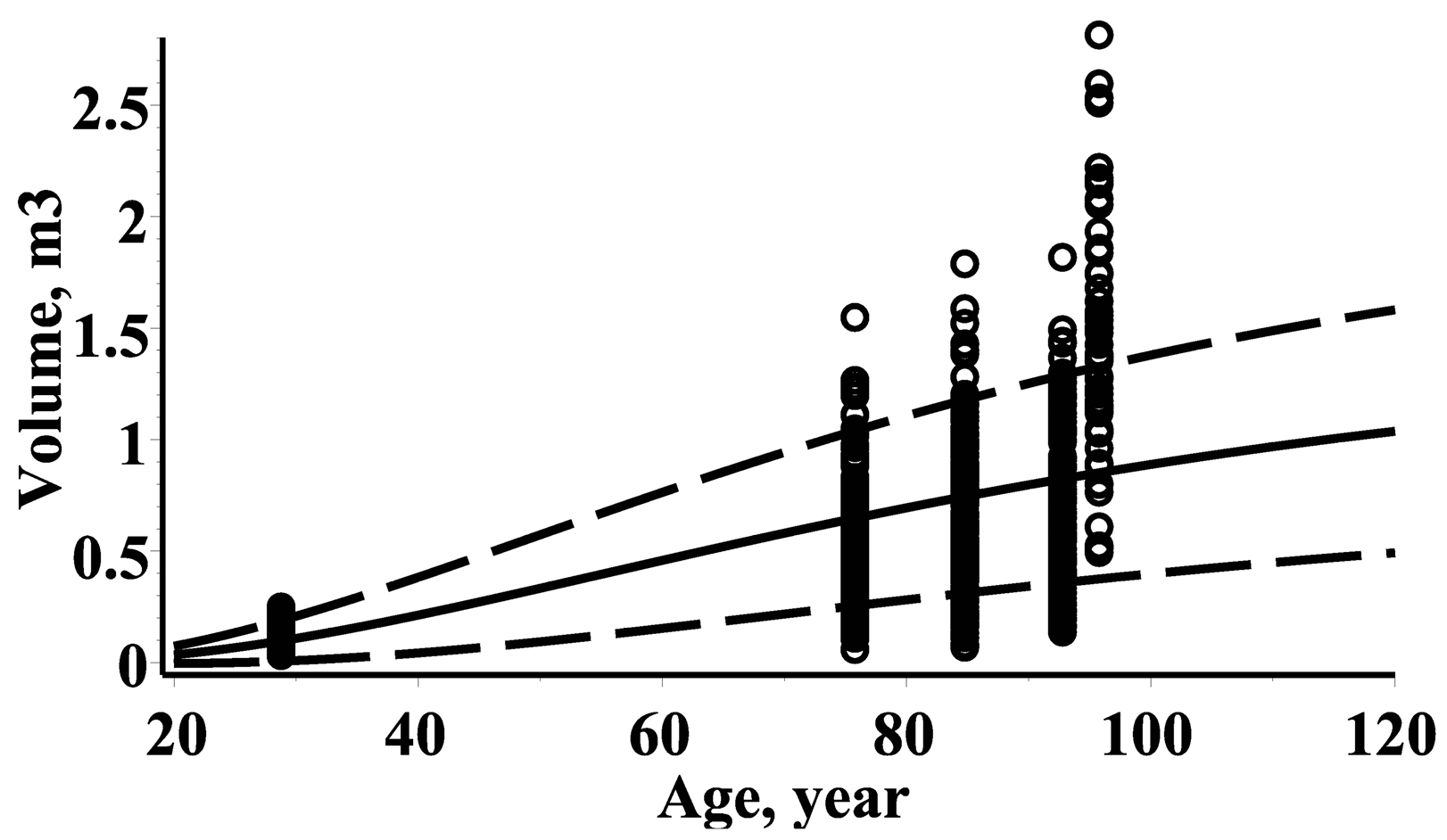
3.6. Mean and Standard Deviation of Stem Volume

The most commonly used mathematical tasks in forestry are quantifying approaches for modeling forest stand dynamics, growth, and yield such as mean tree diameter, height, and stem volume. By using the marginal bivariate probability density functions defined by Equations (15) and (16), the evolution of the mean stem volume and its standard deviation can be defined as, respectively:

$$\overline{V}(t)={\displaystyle \underset{-\infty }{\overset{+\infty }{\int }}{\displaystyle \underset{-\infty }{\overset{+\infty }{\int }}V(x_1,x_2)\cdot f\left(x_1,x_2,t|{\stackrel{\wedge }{\alpha }}_1,{\stackrel{\wedge }{\alpha }}_2,{\stackrel{\wedge }{\beta }}_1,{\stackrel{\wedge }{\beta }}_2,{\stackrel{\wedge }{\sigma }}_{11},{\stackrel{\wedge }{\sigma }}_{22},{\stackrel{\wedge }{\alpha }}_{12}\right)\cdot d{x}_1\cdot d{x}_2}},$$

(32)

$$SD(t)=\sqrt{\overline{V^2}(t)-{\overline{V}}^2(t)},$$

(33)

where

$$\overline{V^2}(t)={\displaystyle \underset{-\infty }{\overset{+\infty }{\int }}{\displaystyle \underset{-\infty }{\overset{+\infty }{\int }}{\left(V(x_1,x_2)\right)}^2\cdot f\left(x_1,x_2,t|{\stackrel{\wedge }{\alpha }}_1,{\stackrel{\wedge }{\alpha }}_2,{\stackrel{\wedge }{\beta }}_1,{\stackrel{\wedge }{\beta }}_2,{\stackrel{\wedge }{\sigma }}_{11},{\stackrel{\wedge }{\sigma }}_{22},{\stackrel{\wedge }{\alpha }}_{12}\right)\cdot d{x}_1\cdot d{x}_2}}.$$

In this study, $V(x_1,x_2)$ is the individual stem volume regression function of a power form, $V(d,h)={\beta }_1{d}^{{\beta }_2}{h}^{{\beta }_3}$, with estimates of the parameters ${\stackrel{\wedge }{\beta }}_1=5.8{*10}^{-5}\hspace{0.17em}(5.8{*10}^{-6})$, ${\stackrel{\wedge }{\beta }}_2=1.8801\hspace{0.17em}(0.028)$, and ${\stackrel{\wedge }{\beta }}_3=0.9723\hspace{0.17em}(0.045)$ [23].

The estimated evolution of the mean stem volume and its standard deviation is shown in Figure 5 with an observed dataset of stem volumes. The observed stem volumes for all trees from the validation dataset were calculated using the power form regression equation $V(x_1,x_2)$.

4. Conclusions

An examination of all newly developed models showed that: in the modeling of the tree diameter, the largest contribution arises from the tree height (one predictor) and from the tree height and crown width (two predictors); in the modeling of the tree height, the largest contribution arises from the tree diameter (one predictor) and from the tree diameter and crown base height (two predictors); in the modeling of the tree crown base height, the largest contribution arises from the tree height (one predictor) and from the tree height and crown width (two predictors); and in the modeling of the tree crown width, the largest contribution arises from the tree diameter (one predictor) and from the tree diameter and crown base height (two predictors).

On the basis of our new developed 4-variate normal distribution, and its marginal trivariate, bivariate, univariate, and conditional univariate distributions, this study provides multiple scientifically reasonable models for the mean and standard deviation dynamics of tree size components and stand attributes, such as the mean stem volume, coefficients of slenderness, and correlation.

In reality, most forest statisticians are focused on the modeling of one single tree size component, and are thus working with one single tree size component trajectory. The models analyzed here in a single response variable scenario could be extended in a number of interesting ways. We considered conditional univariate random variables defined by a tree size component conditioned to give values of other predictor variables that were univariate normally distributed, but these models can be formulated with responses such as those which are bivariate or trivariate. It is obvious that without knowing the underlying covariance structure driving changes in tree size components via age, we cannot appropriately identify predictor variables.

In order to account for stand-to-stand variability in the datasets (see Figure 1, Figure 4 and Figure 5), using a fixed effect modeling technique could be extended to mixed effect models.

References

1. Krainovic, P.; Almeida, D.; Sampaio, P. New allometric equations to support sustainable plantation management of rosewood (Aniba rosaeodora Ducke) in the Central Amazon. Forests 2017, 8, 327. [Google Scholar] [CrossRef]
2. King, D.A. Size-related changes in tree proportions and their potential influence on the course of height growth. In Size- and Age-Related Changes in Tree Structure and Function; Meinzer, F.C., Lachenbruch, B., Dawson, T.E., Eds.; Springer: Dordrecht, The Netherlands, 2011; pp. 165–191. [Google Scholar]
3. Von Gadow, K.; Zhang, C.Y.; Wehenkel, C.; Pommerening, A.; Corral-Rivas, J.; Korol, M.; Myklush, S.; Hui, G.Y.; Kiviste, A.; Zhao, X.H. Forest structure and diversity. In Continuous Cover Forestry; Pukkala, T., Von Gadow, K., Eds.; Springer: Dordrecht, The Netherlands, 2012; pp. 29–83. [Google Scholar]
4. Mirzaei, M.; Aziz, J.; Mahdavi, A.; Rad, A.M. Modeling frequency distributions of tree height, diameter and crown area by six probability functions for open forests of Quercus persica in Iran. J. For. Res. 2015, 27, 901–906. [Google Scholar] [CrossRef]
5. Mohammadalizadeh, A.K.; Namiranian, M.; Zobeiri, M.; Abd-alhosein, H.; Marvie Mohajer, M.R. Modeling of frequency distribution of tree’s height in uneven-aged stands (Case study: Gorazbon district of Khyroud forest). J. For. Wood Prod. 2013, 66, 155–165. [Google Scholar]
6. Gorgoso-Varela, J.J.; García-Villabrille, J.D.; Rojo-Alboreca, A.; von Gadow, K.; Álvarez-González, J.G. Comparing Johnson’s SBB, Weibull and Logit-Logistic bivariate distributions for modeling tree diameters and heights using copulas. For. Syst. 2016, 25, 1–5. [Google Scholar] [CrossRef]
7. Møller, J.K.; Madsen, H.; Carstensen, J. Parameter estimation in a simple stochastic differential equation for phytoplankton modelling. Ecol. Model. 2011, 222, 1793–1799. [Google Scholar] [CrossRef]
8. Rupšys, P. The use of copulas to practical estimation of multivariate stochastic differential equation mixed effects models. AIP Conf. Proc. 2015, 1684, 80011. [Google Scholar] [CrossRef]
9. Cai, W.; Pan, J. Stochastic differential equation models for the price of European CO2 Emissions Allowances. Sustainability 2017, 9, 207. [Google Scholar] [CrossRef]
10. Rupšys, P.; Petrauskas, E. Analysis of height curves by stochastic differential equations. Int. J. Biomath. 2012, 5, 1–15. [Google Scholar] [CrossRef]
11. Rupšys, P. Generalized fixed-effects and mixed-effects parameters height–diameter models with diffusion processes. Int. J. Biomath. 2015, 8, 1–23. [Google Scholar] [CrossRef]
12. Rupšys, P. New insights into tree height distribution based on mixed effects univariate diffusion processes. PLoS ONE 2016, 11, e0168507. [Google Scholar] [CrossRef] [PubMed]
13. Petrauskas, E.; Bartkevičius, E.; Rupšys, P.; Memgaudas, R. The use of stochastic differential equations to describe stem taper and volume. Balt. For. 2013, 19, 43–151. [Google Scholar]
14. Rupšys, P. Stochastic mixed-effects parameters Bertalanffy process, with applications to tree crown width modeling. Math. Probl. Eng. 2015, 2015, 1–10. [Google Scholar] [CrossRef]
15. Itô, K. On stochastic processes. Jpn. J. Math. 1942, 18, 261–301. [Google Scholar] [CrossRef]
16. Arnold, L. Stochastic Differential Equations; John Wiley and Sons: New York, NY, USA, 1973. [Google Scholar]
17. Uhlenbeck, G.E.; Ornstein, L.S. On the theory of Brownian motion. Phys. Rev. 1930, 36, 823–841. [Google Scholar] [CrossRef]
18. Tong, Y.L. The Multivariate Normal Distribution; Springer Series in Statistics; Springer-Verlag: New York, NY, USA, 1990. [Google Scholar]
19. Monagan, M.B.; Geddes, K.O.; Heal, K.M.; Labahn, G.; Vorkoetter, S.M.; Mccarron, J. Maple Advanced Programming Guide; Maplesoft: Waterloo, ON, Canada, 2007. [Google Scholar]
20. Rupšys, P.; Petrauskas, E. A new paradigm in modelling the evolution of a stand via the distribution of tree sizes. Sci. Rep. 2017, 7, 15875. [Google Scholar] [CrossRef] [PubMed]
21. Uria-Diez, J.; Pommerening, A. Crown plasticity in Scots pine (Pinus sylvestris L.) as a strategy ofadaptation to competition and environmental factors. Ecol. Model. 2017, 356, 117–126. [Google Scholar] [CrossRef]
22. Temesgen, H.; LeMay, V.; Mitchell, S.J. Tree crown ratio models for multi-species and multi-layered stands of southeastern British Columbia. For. Chron. 2005, 81, 133–141. [Google Scholar] [CrossRef]
23. Petrauskas, E.; Rupšys, P. The Generalised height-diameter equations of Scots pine (Pinus sylvestris L.) trees in Lithuania. Rural Dev. 2013, 6, 407–411. [Google Scholar]
Figure 1. Observed datasets: (a1) Estimation dataset of diameters; (a2) Validation dataset of diameters; (b1) Estimation dataset of heights; (b2) Validation dataset of heights; (c1) Estimation dataset of crown base heights; (c2) Validation dataset of crown base heights; (d1) Estimation dataset of crown widths; (d2) Validation dataset of crown widths.
Forests 08 00479 g001
Figure 2. Estimated marginal bivariate density functions and their 95% confidence regions with observed datasets from validation datasets: (a1,a2) Diameter and height for the first stand; (b1,b2) Diameter and crown base height for the second stand; (c1,c2) Diameter and crown width for the third stand; (d1,d2) Height and crown base height for the fourth stand; (e1,e2) Height and crown width for the fifth stand; (f1,f2) Crown base height and crown width for the first stand.
Forests 08 00479 g002aForests 08 00479 g002b
Figure 3. Coefficient of correlation among tree size components: between diameter and height–solid line; between diameter and crown base height—dotted line; between diameter and crown width dash line; between height and crown base height—dashdot; between height and crown width—longdash; between crown base height and crown width—spacedash.
Forests 08 00479 g003
Figure 4. Coefficients of slenderness: (a) Slenderness of stem with observed dataset; (b) Slenderness of crown with observed dataset; (c) Competition index with observed dataset.
Forests 08 00479 g004
Figure 5. Mean stem volume and its standard deviation: mean stem volume—solid line; mean stem volume ± standard deviation—dash line; observed stem volumes—circles.
Forests 08 00479 g005