
Carbon Dynamics of Pinus palustris Ecosystems Following Drought

 ,
,  , ,
, ,
Abstract
:1. Introduction
2. Materials and Methods
2.1. Study Sites
2.2. Eddy Covariance Methodology
2.3. Meteorological Instrumentation and Data
2.4. Data Processing
2.5. Data Analyses
3. Results
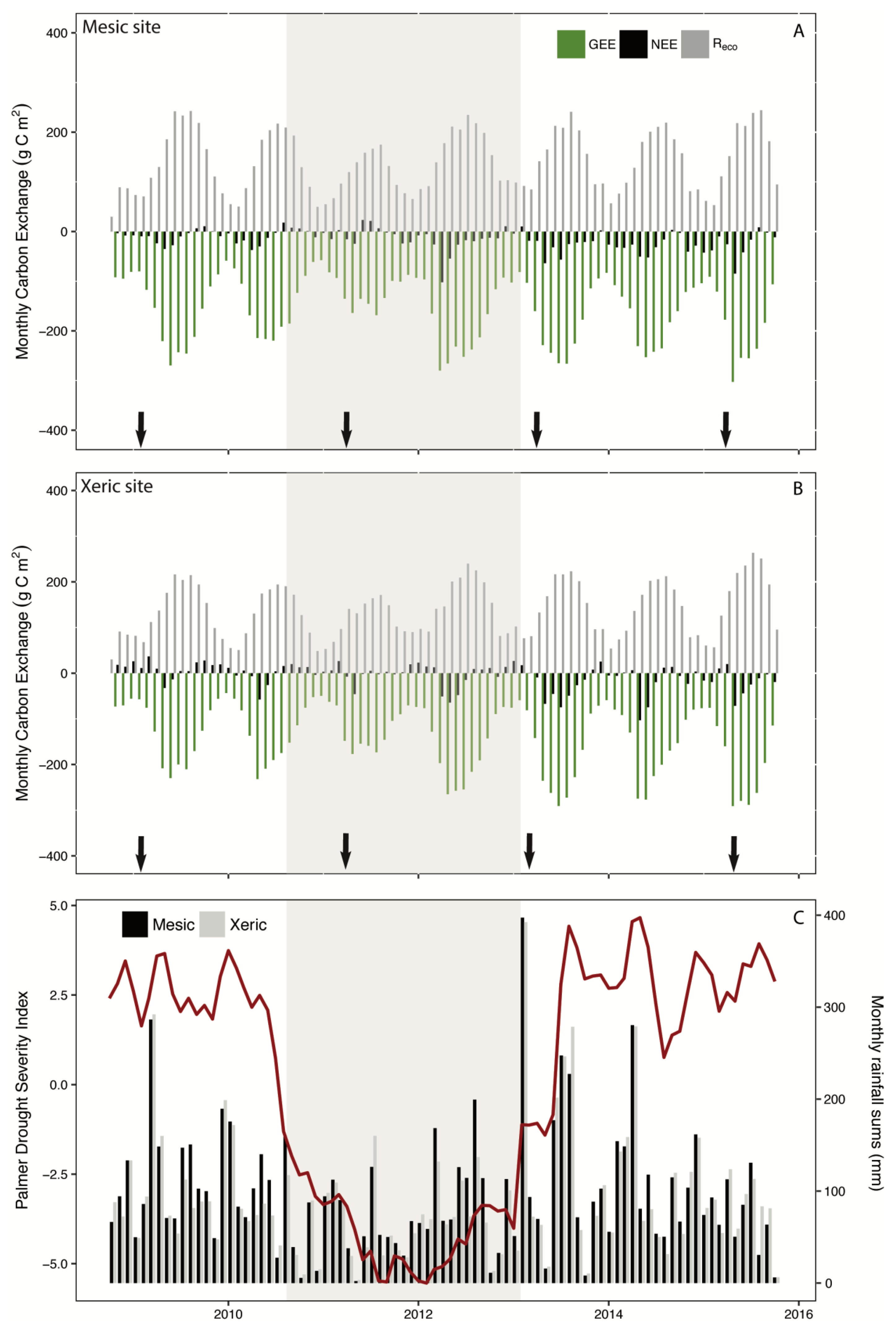
3.1. Micrometerological Conditions
3.2. Annual Carbon
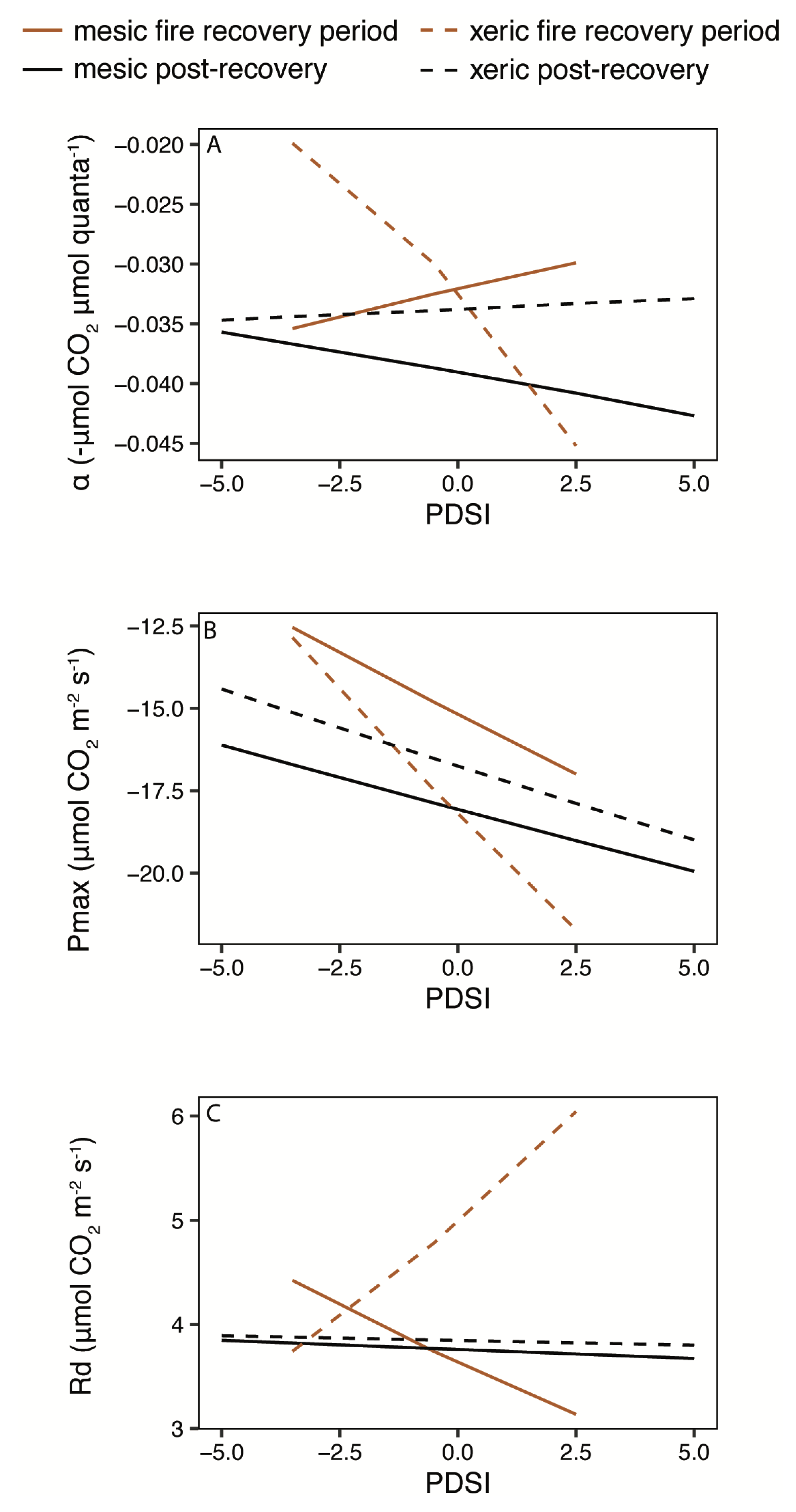
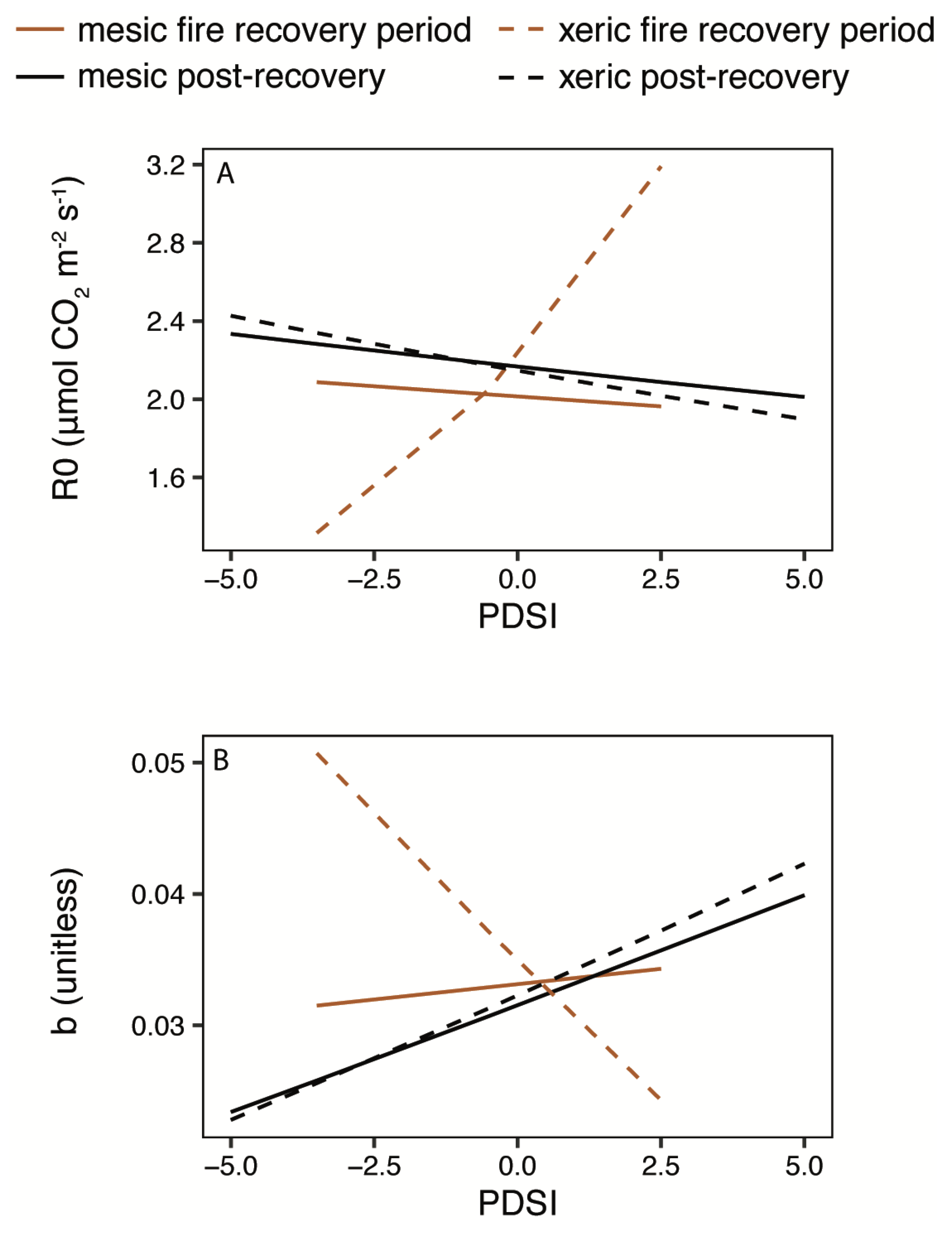
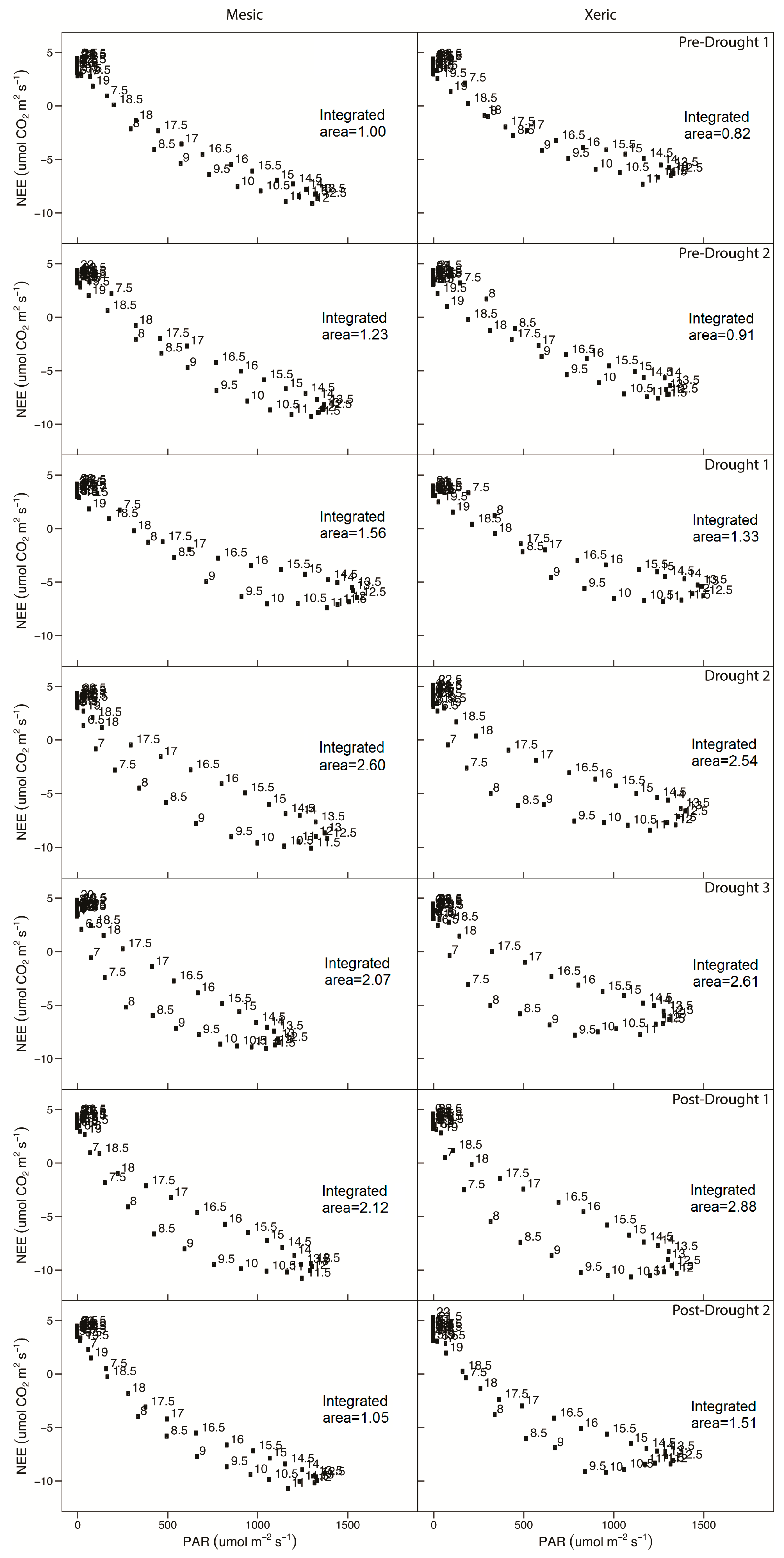
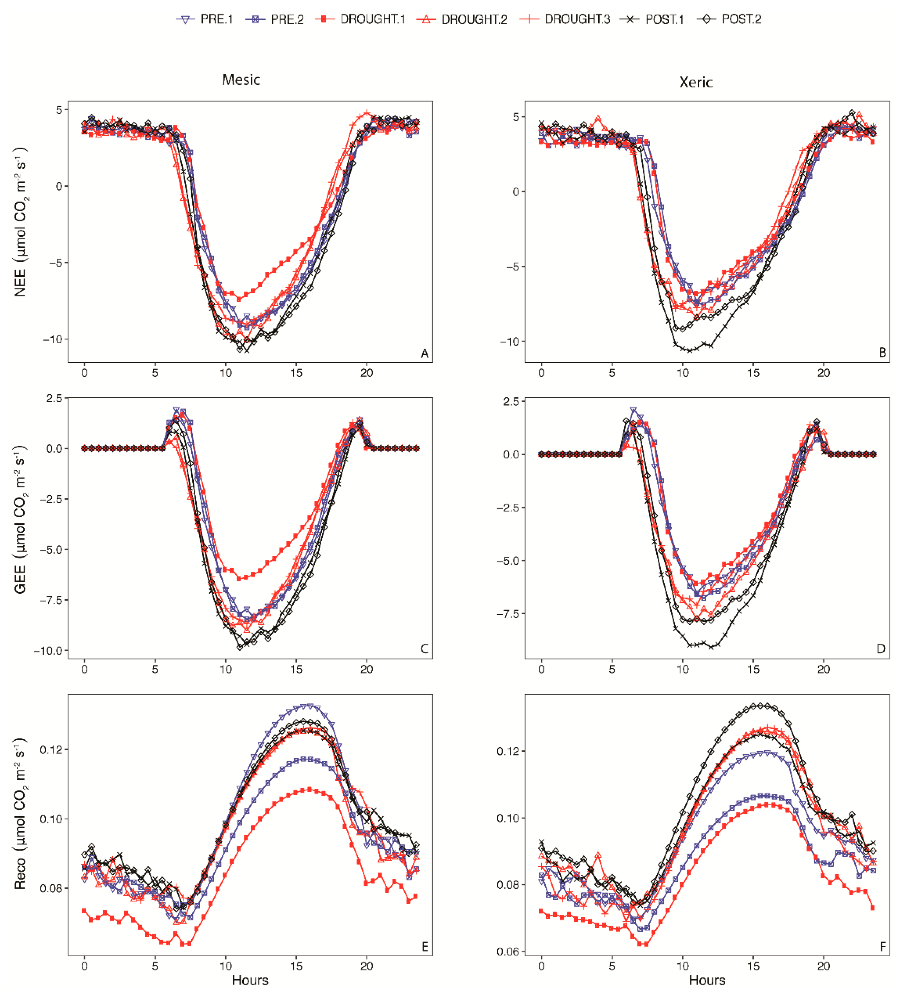
3.3. Light and Temperature Responses Following Drought
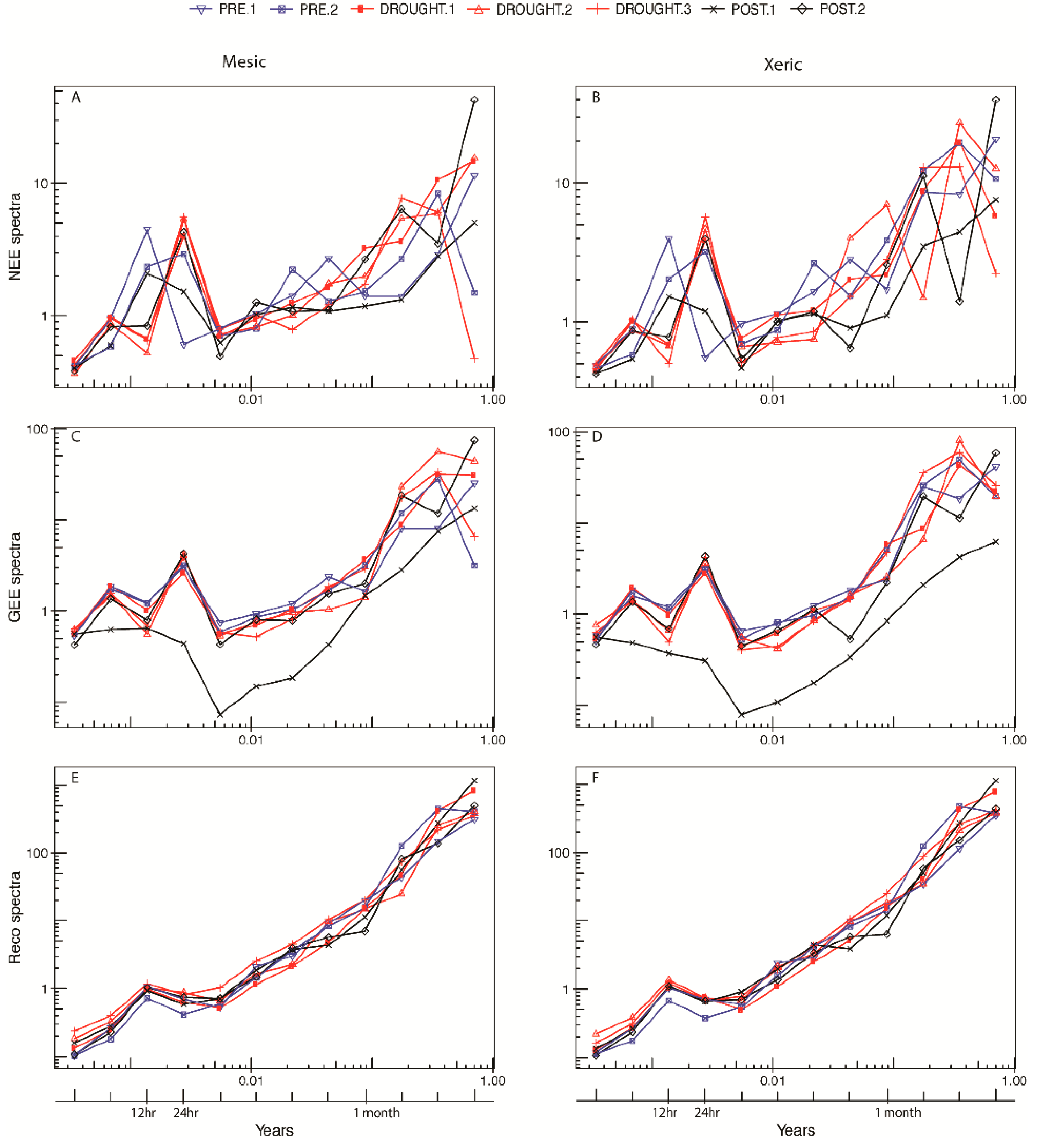
3.4. Orthonormal Wavelet Analyses
3.5. NEE Activity
4. Discussion
4.1. Disturbance and Recovery
4.1.1. Fire
4.1.2. Drought
5. Conclusions
Acknowledgments
Author Contributions
Conflicts of Interest
Abbreviations
| α | Apparent quantum efficiency |
| Ø | Photosynthetically active radiation |
| GEE | Gross ecosystem exchange of carbon |
| GLM | General linear model |
| GPP | Gross primary production |
| IRGA | Infrared Gas Analyzer |
| NEE | Net ecosystem exchange of carbon |
| NEEday | Net ecosystem exchange of carbon during daylight hours |
| NEEnight | Net ecosystem exchange of carbon during night time house |
| NEP | Net ecosystem production |
| NPP | Net primary production |
| OWT | Orthonormal wavelet transformation |
| PAR | Photosynthetically active radiation |
| PDSI | Palmer Drought Severity Index |
| Pmax | Maximum photosynthesis |
| Reco | Ecosystem Respiration |
| Rd | Ecosystem Respiration |
| R0 | Respiration when air temperature is zero |
| SEUS | Southeastern United States |
| Tair | Air temperature |
| U* | Frictional velocity |
| VPD | Vapor pressure deficit |
Appendix A

| α | Pmax | Rd | |||||||||
|---|---|---|---|---|---|---|---|---|---|---|---|
| Site | Year | Month | Estim. Param. | LCL | UCL | Estim. Param. | LCL | UCL | Estim. Param. | LCL | UCL |
| Mesic | 2008 | 10 | −0.033 | −0.058 | −0.013 | −19.14 | −34.95 | −14.99 | 3.350 | 0.786 | 5.452 |
| 11 | −0.031 | −0.041 | −0.024 | −12.26 | −13.45 | −11.43 | 2.831 | 2.378 | 3.424 | ||
| 12 | −0.038 | −0.049 | −0.029 | −12.37 | −13.46 | −11.54 | 2.483 | 1.998 | 3.029 | ||
| 2009 | 1 | −0.029 | −0.042 | −0.021 | −9.00 | −10.01 | −8.22 | 1.946 | 1.443 | 2.503 | |
| 2 | −0.016 | −0.020 | −0.012 | −15.12 | −17.81 | −13.55 | 2.524 | 1.973 | 3.119 | ||
| 3 | −0.014 | −0.019 | −0.010 | −17.70 | −22.49 | −15.34 | 2.074 | 1.485 | 2.837 | ||
| 4 | −0.029 | −0.036 | −0.024 | −16.32 | −17.36 | −15.48 | 4.033 | 3.403 | 4.835 | ||
| 5 | −0.048 | −0.058 | −0.040 | −22.72 | −23.92 | −21.70 | 5.953 | 5.083 | 6.787 | ||
| 6 | −0.053 | −0.071 | −0.041 | −21.89 | −23.67 | −20.54 | 6.749 | 5.389 | 8.440 | ||
| 7 | −0.053 | −0.070 | −0.042 | −26.50 | −28.08 | −25.03 | 9.014 | 7.570 | 10.645 | ||
| 8 | −0.043 | −0.054 | −0.034 | −26.16 | −28.18 | −24.49 | 6.849 | 5.687 | 8.060 | ||
| 9 | −0.051 | −0.062 | −0.043 | −27.21 | −28.84 | −25.81 | 7.835 | 6.762 | 9.084 | ||
| 10 | −0.038 | −0.045 | −0.032 | −23.98 | −25.78 | −22.54 | 5.358 | 4.539 | 6.196 | ||
| 11 | −0.034 | −0.050 | −0.023 | −20.59 | −23.66 | −18.90 | 4.035 | 2.690 | 5.640 | ||
| 12 | −0.030 | −0.038 | −0.025 | −18.03 | −20.32 | −16.47 | 2.520 | 1.867 | 3.332 | ||
| 2010 | 1 | −0.035 | −0.071 | −0.017 | −6.63 | −7.85 | −5.85 | 2.271 | 1.372 | 3.619 | |
| 2 | −0.043 | −0.057 | −0.032 | −9.37 | −10.31 | −8.62 | 2.568 | 1.879 | 3.447 | ||
| 3 | −0.018 | −0.023 | −0.015 | −12.62 | −13.64 | −11.73 | 2.255 | 1.760 | 2.912 | ||
| 4 | −0.022 | −0.027 | −0.017 | −21.07 | −23.65 | −19.52 | 4.192 | 3.530 | 4.913 | ||
| 5 | −0.033 | −0.040 | −0.028 | −27.49 | −29.50 | −25.71 | 6.550 | 5.611 | 7.621 | ||
| 6 | −0.034 | −0.045 | −0.026 | −23.46 | −25.50 | −21.85 | 6.794 | 5.537 | 8.279 | ||
| 7 | −0.036 | −0.047 | −0.028 | −18.08 | −19.62 | −16.86 | 5.791 | 5.030 | 6.666 | ||
| 8 | −0.047 | −0.062 | −0.036 | −19.95 | −21.54 | −18.46 | 7.236 | 6.164 | 8.518 | ||
| 9 | −0.025 | −0.035 | −0.020 | −22.52 | −25.43 | −20.20 | 5.555 | 4.461 | 7.146 | ||
| 10 | −0.015 | −0.023 | −0.011 | −15.34 | −19.28 | −13.55 | 3.176 | 2.275 | 4.199 | ||
| 11 | −0.034 | −0.056 | −0.023 | −14.43 | −16.55 | −12.87 | 4.238 | 2.884 | 6.174 | ||
| 12 | −0.010 | −0.014 | −0.007 | −12.21 | −19.32 | −9.21 | 1.168 | 0.808 | 1.519 | ||
| 2011 | 1 | −0.025 | −0.041 | −0.015 | −9.67 | −11.38 | −8.37 | 2.586 | 1.402 | 4.079 | |
| 2 | −0.021 | −0.028 | −0.016 | −12.99 | −14.80 | −11.93 | 2.359 | 1.901 | 2.910 | ||
| 3 | −0.044 | −0.066 | −0.031 | −12.20 | −14.02 | −10.89 | 4.917 | 3.769 | 6.646 | ||
| 4 | −0.022 | −0.030 | −0.018 | −16.19 | −17.75 | −15.09 | 4.259 | 3.554 | 5.128 | ||
| 5 | −0.025 | −0.032 | −0.020 | −13.42 | −14.55 | −12.56 | 3.715 | 3.263 | 4.237 | ||
| 6 | −0.035 | −0.049 | −0.026 | −9.09 | −9.95 | −8.26 | 4.435 | 3.771 | 5.207 | ||
| 7 | −0.026 | −0.034 | −0.020 | −16.81 | −18.62 | −15.63 | 5.841 | 5.048 | 6.918 | ||
| 8 | −0.030 | −0.049 | −0.021 | −19.53 | −22.24 | −17.75 | 6.467 | 4.997 | 8.967 | ||
| 9 | −0.032 | −0.048 | −0.021 | −11.63 | −13.14 | −10.54 | 3.120 | 2.232 | 4.168 | ||
| 10 | −0.021 | −0.035 | −0.011 | −11.02 | −13.87 | −9.63 | 3.379 | 2.409 | 4.580 | ||
| 11 | −0.015 | −0.019 | −0.013 | −22.73 | −29.40 | −19.05 | 2.159 | 1.783 | 2.583 | ||
| 12 | −0.019 | −0.028 | −0.013 | −16.07 | −21.85 | −13.72 | 1.581 | 0.973 | 2.482 | ||
| 2012 | 1 | −0.025 | −0.042 | −0.017 | −11.59 | −13.40 | −10.48 | 2.458 | 1.460 | 3.921 | |
| 2 | −0.044 | −0.083 | −0.027 | −15.30 | −17.97 | −13.30 | 4.109 | 2.431 | 7.206 | ||
| 3 | −0.062 | −0.090 | −0.045 | −13.94 | −15.10 | −13.01 | 4.302 | 3.414 | 5.459 | ||
| 4 | −0.079 | −0.128 | −0.048 | −27.28 | −29.82 | −25.39 | 5.871 | 3.339 | 8.527 | ||
| 5 | −0.153 | −0.304 | −0.087 | −18.91 | −24.12 | −15.40 | 7.048 | 3.415 | 12.038 | ||
| 6 | −0.096 | −0.171 | −0.061 | −19.25 | −22.10 | −17.26 | 7.553 | 5.483 | 10.503 | ||
| 7 | −0.096 | −0.203 | −0.055 | −17.60 | −21.03 | −15.43 | 6.953 | 4.572 | 10.747 | ||
| 8 | −0.087 | −0.161 | −0.050 | −19.23 | −21.87 | −16.95 | 6.299 | 3.913 | 9.116 | ||
| 9 | −0.105 | −0.210 | −0.058 | −20.80 | −24.75 | −17.20 | 7.981 | 4.331 | 12.321 | ||
| 10 | −0.061 | −0.107 | −0.031 | −14.92 | −16.76 | −13.62 | 3.625 | 1.687 | 5.493 | ||
| 11 | −0.026 | −0.038 | −0.019 | −17.24 | −21.28 | −15.20 | 2.117 | 1.377 | 3.138 | ||
| 12 | −0.054 | −0.129 | −0.030 | −15.71 | −18.59 | −13.87 | 4.531 | 2.535 | 8.494 | ||
| 2013 | 1 | −0.029 | −0.036 | −0.024 | −17.65 | −20.07 | −16.12 | 2.708 | 2.082 | 3.349 | |
| 2 | −0.034 | −0.046 | −0.027 | −13.34 | −14.74 | −12.39 | 2.630 | 2.076 | 3.291 | ||
| 3 | −0.024 | −0.039 | −0.015 | −8.42 | −9.67 | −7.52 | 1.607 | 0.733 | 2.379 | ||
| 4 | −0.043 | −0.080 | −0.025 | −11.38 | −12.91 | −10.20 | 2.135 | 0.914 | 3.643 | ||
| 5 | −0.088 | −0.181 | −0.045 | −15.56 | −18.57 | −13.37 | 4.590 | 1.948 | 7.711 | ||
| 6 | −0.151 | −0.261 | −0.092 | −19.18 | −22.25 | −16.79 | 7.706 | 5.226 | 10.989 | ||
| 7 | −0.152 | −0.299 | −0.085 | −20.91 | −24.52 | −18.15 | 7.193 | 4.006 | 11.078 | ||
| 8 | −0.182 | −0.395 | −0.096 | −20.90 | −26.94 | −17.15 | 8.180 | 4.176 | 14.139 | ||
| 9 | −0.169 | −0.414 | −0.077 | −20.37 | −26.88 | −16.87 | 8.283 | 4.212 | 14.916 | ||
| 10 | −0.202 | −0.495 | −0.100 | −22.16 | −29.25 | −18.06 | 10.463 | 5.778 | 17.891 | ||
| 11 | −0.033 | −0.041 | −0.027 | −17.78 | −19.41 | −16.44 | 2.605 | 2.089 | 3.173 | ||
| 12 | −0.040 | −0.057 | −0.029 | −13.53 | −15.13 | −12.22 | 2.808 | 1.795 | 3.919 | ||
| 2014 | 1 | −0.026 | −0.057 | −0.013 | −7.14 | −8.60 | −6.19 | 0.134 | -0.686 | 1.437 | |
| 2 | −0.023 | −0.046 | −0.011 | −10.64 | −13.75 | −9.32 | -0.062 | -1.214 | 1.507 | ||
| 3 | −0.025 | −0.037 | −0.017 | −15.05 | −17.06 | −13.61 | 1.987 | 0.868 | 3.183 | ||
| 4 | −0.039 | −0.056 | −0.028 | −15.48 | −16.86 | −14.44 | 3.364 | 2.355 | 4.646 | ||
| 5 | −0.046 | −0.060 | −0.036 | −23.31 | −25.03 | −21.91 | 6.465 | 5.260 | 8.042 | ||
| 6 | −0.042 | −0.055 | −0.034 | −23.38 | −25.28 | −21.94 | 5.670 | 4.667 | 7.062 | ||
| 7 | −0.046 | −0.060 | −0.036 | −24.54 | −26.48 | −22.98 | 7.242 | 5.905 | 8.859 | ||
| 8 | −0.047 | −0.065 | −0.035 | −18.38 | −19.88 | −17.16 | 5.169 | 4.084 | 6.460 | ||
| 9 | −0.046 | −0.064 | −0.034 | −19.89 | −21.93 | −18.13 | 5.131 | 3.761 | 6.770 | ||
| 10 | −0.017 | −0.023 | −0.013 | −25.93 | −33.96 | −21.91 | 2.897 | 2.020 | 3.830 | ||
| 11 | −0.023 | −0.045 | −0.012 | −13.24 | −19.04 | −11.45 | 0.019 | -1.255 | 1.426 | ||
| 12 | −0.018 | −0.040 | −0.008 | −15.83 | −44.43 | −12.32 | -0.399 | -1.923 | 1.581 | ||
| 2015 | 1 | −0.021 | −0.035 | −0.013 | −11.40 | −14.17 | −10.06 | -0.333 | -1.156 | 0.602 | |
| 2 | −0.022 | −0.037 | −0.013 | −8.50 | −10.12 | −7.48 | -0.183 | -0.994 | 0.697 | ||
| 3 | −0.032 | −0.043 | −0.024 | −11.61 | −12.72 | −10.62 | 2.724 | 2.031 | 3.409 | ||
| 4 | −0.052 | −0.067 | −0.040 | −22.27 | −24.06 | −20.92 | 5.706 | 4.669 | 6.805 | ||
| 5 | −0.049 | −0.064 | −0.038 | −37.80 | −41.38 | −35.35 | 8.079 | 6.530 | 9.892 | ||
| 6 | −0.043 | −0.058 | −0.033 | −21.70 | −23.54 | −20.17 | 5.588 | 4.404 | 6.881 | ||
| 7 | −0.065 | −0.088 | −0.049 | −20.32 | −22.00 | −18.95 | 7.405 | 6.099 | 9.099 | ||
| 8 | −0.048 | −0.065 | −0.035 | −21.05 | −22.93 | −19.52 | 6.586 | 5.165 | 8.288 | ||
| 9 | −0.059 | −0.079 | −0.045 | −19.55 | −21.10 | −18.29 | 6.043 | 5.010 | 7.345 | ||
| 10 | −0.055 | −0.070 | −0.042 | −15.14 | −16.32 | −13.99 | 4.274 | 3.479 | 5.176 | ||
| Xeric | 2008 | 12 | −0.012 | −0.021 | −0.007 | −9.21 | −17.16 | −7.55 | 1.474 | 0.827 | 2.214 |
| 2009 | 1 | −0.015 | −0.025 | −0.010 | −6.18 | −7.35 | −5.56 | 1.989 | 1.575 | 2.488 | |
| 2 | −0.012 | −0.022 | −0.007 | −6.68 | −8.26 | −5.95 | 2.009 | 1.432 | 2.828 | ||
| 3 | −0.014 | −0.019 | −0.011 | −10.02 | −11.63 | −8.87 | 3.339 | 2.802 | 3.994 | ||
| 4 | −0.031 | −0.043 | −0.023 | −13.02 | −14.36 | −12.02 | 4.338 | 3.525 | 5.413 | ||
| 5 | −0.054 | −0.065 | −0.046 | −22.86 | −24.08 | −21.81 | 6.631 | 5.834 | 7.523 | ||
| 6 | −0.054 | −0.074 | −0.042 | −20.57 | −22.33 | −19.27 | 7.098 | 6.046 | 8.747 | ||
| 7 | −0.047 | −0.059 | −0.038 | −22.20 | −23.86 | −20.88 | 8.322 | 7.136 | 9.710 | ||
| 8 | −0.039 | −0.056 | −0.029 | −27.53 | −30.37 | −25.30 | 7.648 | 5.851 | 10.090 | ||
| 9 | −0.038 | −0.049 | −0.030 | −21.44 | −22.99 | −20.19 | 6.338 | 5.251 | 7.672 | ||
| 10 | −0.036 | −0.044 | −0.029 | −20.10 | −21.86 | −18.79 | 5.611 | 4.731 | 6.608 | ||
| 11 | −0.018 | −0.030 | −0.011 | −15.20 | −21.18 | −13.12 | 2.823 | 1.925 | 3.966 | ||
| 12 | −0.022 | −0.032 | −0.016 | −10.68 | −12.22 | −9.64 | 2.511 | 1.962 | 3.334 | ||
| 2010 | 1 | −0.024 | −0.045 | −0.013 | −4.07 | −4.72 | −3.58 | 1.811 | 1.248 | 2.485 | |
| 2 | −0.024 | −0.032 | −0.019 | −6.27 | −6.74 | −5.86 | 1.827 | 1.494 | 2.205 | ||
| 3 | −0.005 | −0.008 | −0.004 | −15.58 | −36.64 | −10.22 | 1.053 | 0.748 | 1.437 | ||
| 4 | −0.009 | −0.014 | −0.006 | −25.19 | −68.63 | −17.57 | 2.483 | 1.640 | 3.554 | ||
| 5 | −0.032 | −0.043 | −0.024 | −28.86 | −32.57 | −26.43 | 5.123 | 3.916 | 6.699 | ||
| 6 | −0.032 | −0.047 | −0.023 | −18.48 | −20.77 | −16.79 | 4.730 | 3.512 | 6.422 | ||
| 7 | −0.033 | −0.044 | −0.026 | −18.34 | −20.21 | −16.97 | 6.246 | 5.387 | 7.359 | ||
| 8 | −0.042 | −0.055 | −0.034 | −19.00 | −20.63 | −17.68 | 6.748 | 5.905 | 7.781 | ||
| 9 | −0.017 | −0.021 | −0.014 | −16.93 | −19.57 | −14.88 | 3.902 | 3.209 | 4.747 | ||
| 10 | −0.017 | −0.024 | −0.012 | −15.05 | −17.65 | −13.48 | 3.576 | 2.675 | 4.764 | ||
| 11 | −0.025 | −0.049 | −0.015 | −13.03 | −14.96 | −11.84 | 3.816 | 2.566 | 5.900 | ||
| 12 | −0.006 | −0.009 | −0.005 | −15.33 | −48.02 | −9.23 | 0.981 | 0.752 | 1.238 | ||
| 2011 | 1 | −0.016 | −0.025 | −0.010 | −6.13 | −7.02 | −5.57 | 1.431 | 0.943 | 2.054 | |
| 2 | −0.010 | −0.014 | −0.006 | −10.81 | −16.78 | −9.21 | 1.518 | 0.931 | 2.151 | ||
| 3 | −0.021 | −0.032 | −0.014 | −8.39 | −9.43 | −7.73 | 3.456 | 2.833 | 4.247 | ||
| 4 | −0.025 | −0.032 | −0.020 | −20.79 | −23.63 | −18.76 | 5.250 | 4.472 | 6.125 | ||
| 5 | −0.030 | −0.037 | −0.024 | −16.93 | −18.23 | −15.84 | 4.813 | 4.203 | 5.595 | ||
| 6 | −0.023 | −0.031 | −0.017 | −11.50 | −12.64 | −10.78 | 3.766 | 3.335 | 4.391 | ||
| 7 | −0.027 | −0.036 | −0.021 | −20.18 | −22.38 | −18.44 | 6.117 | 5.195 | 7.403 | ||
| 8 | −0.027 | −0.036 | −0.020 | −19.80 | −22.10 | −17.89 | 5.761 | 4.622 | 7.331 | ||
| 9 | −0.033 | −0.043 | −0.025 | −17.58 | −19.38 | −16.37 | 4.555 | 3.730 | 5.506 | ||
| 10 | −0.016 | −0.027 | −0.010 | −10.15 | −12.43 | −9.19 | 2.028 | 1.357 | 2.844 | ||
| 11 | −0.019 | −0.026 | −0.015 | −13.66 | −16.30 | −12.08 | 2.457 | 1.975 | 3.007 | ||
| 12 | −0.018 | −0.027 | −0.012 | −11.13 | −14.42 | −9.72 | 1.974 | 1.347 | 2.694 | ||
| 2012 | 1 | −0.014 | −0.021 | −0.010 | −10.72 | −14.21 | −8.95 | 2.199 | 1.660 | 2.849 | |
| 2 | −0.021 | −0.032 | −0.015 | −12.09 | −15.09 | −10.33 | 2.748 | 1.876 | 3.618 | ||
| 3 | −0.093 | −0.234 | −0.045 | −10.10 | −13.77 | −8.25 | 5.105 | 3.138 | 8.680 | ||
| 4 | −0.180 | −0.408 | −0.092 | −17.50 | −21.99 | −14.61 | 7.998 | 4.828 | 12.568 | ||
| 5 | −0.216 | −0.445 | −0.129 | −22.10 | −27.27 | −19.11 | 10.342 | 7.272 | 15.437 | ||
| 6 | −0.115 | −0.191 | −0.077 | −20.98 | −23.65 | −18.76 | 7.941 | 5.711 | 10.732 | ||
| 7 | −0.504 | −1.870 | −0.242 | −23.12 | −38.05 | −17.43 | 14.909 | 9.178 | 29.549 | ||
| 8 | −0.187 | −0.331 | −0.119 | −20.90 | −25.06 | −17.65 | 10.896 | 7.723 | 15.181 | ||
| 9 | −0.311 | −0.854 | −0.164 | −28.22 | −39.61 | −22.79 | 17.826 | 12.213 | 28.457 | ||
| 10 | −0.084 | −1.572 | −0.033 | −14.66 | −36.50 | −11.83 | 6.092 | 2.690 | 28.430 | ||
| 11 | −0.017 | −0.027 | −0.011 | −9.09 | −10.83 | −7.99 | 1.251 | 0.648 | 2.012 | ||
| 12 | −0.024 | −0.037 | −0.015 | −8.58 | −10.29 | −7.43 | 1.908 | 1.224 | 2.704 | ||
| 2013 | 1 | −0.016 | −0.022 | −0.011 | −11.59 | −13.84 | −10.32 | 2.339 | 1.741 | 3.032 | |
| 2 | −0.026 | −0.043 | −0.016 | −8.34 | −10.30 | −7.05 | 2.573 | 1.634 | 3.834 | ||
| 3 | −0.020 | −0.040 | −0.012 | −5.66 | −6.81 | −4.95 | 1.737 | 1.021 | 2.905 | ||
| 4 | −0.105 | −0.247 | −0.050 | −10.26 | −13.02 | −8.66 | 4.362 | 2.517 | 7.162 | ||
| 5 | −0.223 | −0.489 | −0.120 | −18.05 | −21.93 | −15.55 | 8.218 | 5.566 | 12.231 | ||
| 6 | −0.111 | −0.207 | −0.066 | −22.09 | −26.03 | −19.11 | 7.914 | 4.706 | 11.945 | ||
| 7 | −0.256 | −1.050 | −0.117 | −26.59 | −40.75 | −20.56 | 11.012 | 5.066 | 25.741 | ||
| 8 | −0.180 | −0.340 | −0.103 | −23.21 | −29.54 | −18.67 | 9.679 | 5.281 | 15.674 | ||
| 9 | −0.090 | −0.172 | −0.054 | −22.92 | −27.16 | −20.13 | 7.815 | 4.655 | 12.269 | ||
| 10 | −0.099 | −0.203 | −0.046 | −18.98 | −22.54 | −16.42 | 7.102 | 3.662 | 11.053 | ||
| 11 | −0.019 | −0.025 | −0.014 | −13.98 | −16.53 | −12.42 | 2.128 | 1.593 | 2.758 | ||
| 12 | −0.021 | −0.032 | −0.015 | −12.90 | −15.88 | −11.23 | 2.640 | 1.827 | 3.602 | ||
| 2014 | 1 | −0.011 | −0.020 | −0.007 | −5.53 | −7.22 | −4.63 | 0.268 | -0.196 | 0.849 | |
| 2 | −0.016 | −0.027 | −0.010 | −5.88 | −7.10 | −5.05 | 0.013 | -0.587 | 0.715 | ||
| 3 | −0.019 | −0.031 | −0.012 | −10.12 | −11.65 | −9.19 | 2.401 | 1.596 | 3.340 | ||
| 4 | −0.039 | −0.054 | −0.029 | −15.93 | −17.48 | −14.83 | 4.908 | 4.037 | 6.021 | ||
| 5 | −0.061 | −0.086 | −0.048 | −29.32 | −32.23 | −27.23 | 7.598 | 6.035 | 10.450 | ||
| 6 | −0.081 | −0.134 | −0.054 | −25.32 | −28.89 | −22.68 | 7.912 | 5.084 | 11.855 | ||
| 7 | −0.078 | −0.123 | −0.056 | −22.26 | −25.65 | −20.01 | 9.357 | 7.118 | 12.822 | ||
| 8 | −0.047 | −0.062 | −0.035 | −12.38 | −13.59 | −11.45 | 4.383 | 3.733 | 5.323 | ||
| 9 | −0.053 | −0.069 | −0.039 | −17.61 | −19.36 | −16.40 | 5.558 | 4.551 | 6.569 | ||
| 10 | −0.020 | −0.026 | −0.015 | −21.61 | −26.40 | −18.81 | 3.116 | 2.414 | 3.946 | ||
| 11 | −0.012 | −0.022 | −0.006 | −13.00 | −61.73 | −9.74 | -0.377 | -1.245 | 0.583 | ||
| 12 | −0.010 | −0.026 | −0.005 | −11.33 | −51.46 | −7.59 | 0.116 | -0.931 | 1.527 | ||
| 2015 | 1 | −0.014 | −0.022 | −0.009 | −8.75 | −11.63 | −7.43 | 0.458 | -0.184 | 1.209 | |
| 2 | −0.013 | −0.021 | −0.008 | −7.70 | −10.54 | −6.56 | 0.084 | -0.468 | 0.652 | ||
| 3 | −0.024 | −0.031 | −0.019 | −12.17 | −13.33 | −11.11 | 2.927 | 2.312 | 3.630 | ||
| 4 | −0.075 | −0.101 | −0.059 | −18.63 | −20.18 | −17.43 | 7.234 | 6.228 | 8.620 | ||
| 5 | −0.072 | −0.096 | −0.056 | −30.90 | −32.96 | −29.14 | 9.824 | 8.189 | 11.787 | ||
| 6 | −0.100 | −0.166 | −0.069 | −27.25 | −31.49 | −24.63 | 11.088 | 8.177 | 15.580 | ||
| 7 | −0.056 | −0.077 | −0.042 | −25.87 | −28.15 | −24.10 | 8.297 | 6.585 | 10.374 | ||
| 8 | −0.052 | −0.071 | −0.039 | −24.96 | −27.33 | −23.23 | 7.596 | 6.271 | 9.254 | ||
| 9 | −0.056 | −0.075 | −0.044 | −23.26 | −25.07 | −21.71 | 6.755 | 5.673 | 8.318 | ||
| 10 | −0.042 | −0.053 | −0.032 | −20.47 | −22.73 | −18.87 | 4.542 | 3.701 | 5.518 | ||
| Annual (yr 1) | -0.020 | −0.020 | −0.021 | −0.018 | −18.66 | −19.67 | −17.88 | 3.462 | 4.002 | ||
| R0 | b | |||||||
|---|---|---|---|---|---|---|---|---|
| Site | Year | Month | Estim. Param. | LCL | UCL | Estim. Param. | LCL | UCL |
| Mesic | 2008 | 10 | 1.455 | 0.090 | 4.705 | 0.038 | −0.022 | 0.185 |
| 11 | 1.318 | 1.099 | 1.566 | 0.048 | 0.035 | 0.061 | ||
| 12 | 1.138 | 1.004 | 1.291 | 0.051 | 0.043 | 0.060 | ||
| 2009 | 1 | 1.180 | 1.063 | 1.307 | 0.046 | 0.039 | 0.053 | |
| 2 | 1.148 | 0.839 | 1.464 | 0.050 | 0.032 | 0.073 | ||
| 3 | 1.315 | 0.994 | 1.613 | 0.052 | 0.039 | 0.068 | ||
| 4 | 1.093 | 0.802 | 1.411 | 0.065 | 0.050 | 0.083 | ||
| 5 | 2.804 | 1.701 | 4.098 | 0.029 | 0.010 | 0.052 | ||
| 6 | 3.349 | 1.598 | 6.993 | 0.022 | −0.007 | 0.051 | ||
| 8 | 1.174 | 0.182 | 6.264 | 0.077 | 0.008 | 0.155 | ||
| 9 | 5.713 | 2.698 | 13.152 | 0.007 | −0.030 | 0.039 | ||
| 10 | 1.828 | 1.385 | 2.253 | 0.052 | 0.042 | 0.066 | ||
| 11 | 2.447 | 1.491 | 3.548 | 0.032 | 0.003 | 0.071 | ||
| 12 | 1.587 | 1.269 | 1.995 | 0.037 | 0.017 | 0.056 | ||
| 2010 | 1 | 0.761 | 0.706 | 0.825 | 0.069 | 0.063 | 0.076 | |
| 2 | 0.816 | 0.715 | 0.912 | 0.068 | 0.058 | 0.081 | ||
| 3 | 1.177 | 0.912 | 1.499 | 0.056 | 0.041 | 0.072 | ||
| 4 | 1.605 | 1.016 | 2.593 | 0.045 | 0.020 | 0.069 | ||
| 5 | 3.049 | 1.462 | 5.304 | 0.026 | 0.0011 | 0.061 | ||
| 11 | 1.162 | 0.687 | 1.556 | 0.059 | 0.039 | 0.095 | ||
| 12 | 0.876 | 0.760 | 1.003 | 0.048 | 0.042 | 0.055 | ||
| 2011 | 1 | 0.577 | 0.264 | 0.889 | 0.115 | 0.076 | 0.180 | |
| 2 | 1.158 | 0.991 | 1.391 | 0.044 | 0.032 | 0.053 | ||
| 3 | 1.559 | 1.120 | 2.034 | 0.037 | 0.021 | 0.058 | ||
| 5 | 1.955 | 1.492 | 2.484 | 0.031 | 0.020 | 0.043 | ||
| 8 | 2.247 | 0.357 | 13.357 | 0.038 | −0.031 | 0.109 | ||
| 9 | 3.678 | 2.493 | 5.354 | 0.0013 | −0.016 | 0.018 | ||
| 10 | 2.293 | 1.605 | 3.013 | 0.0010 | −0.017 | 0.022 | ||
| 11 | 1.441 | 1.199 | 1.792 | 0.021 | 0.007 | 0.033 | ||
| 12 | 1.310 | 1.028 | 1.646 | 0.014 | −0.006 | 0.032 | ||
| 2012 | 1 | 0.795 | 0.615 | 0.969 | 0.071 | 0.048 | 0.093 | |
| 2 | 1.545 | 1.121 | 2.107 | 0.038 | 0.025 | 0.053 | ||
| 3 | 0.913 | 0.526 | 1.331 | 0.068 | 0.045 | 0.097 | ||
| 4 | 2.019 | 0.998 | 3.198 | 0.059 | 0.034 | 0.093 | ||
| 5 | 2.408 | 0.925 | 5.432 | 0.043 | 0.006 | 0.083 | ||
| 9 | 4.660 | 1.178 | 22.594 | 0.016 | −0.055 | 0.070 | ||
| 10 | 1.070 | 0.661 | 1.543 | 0.077 | 0.056 | 0.103 | ||
| 11 | 2.351 | 1.425 | 3.950 | 0.006 | −0.029 | 0.036 | ||
| 12 | 1.718 | 1.249 | 2.215 | 0.045 | 0.028 | 0.067 | ||
| 2013 | 1 | 1.608 | 1.378 | 1.874 | 0.038 | 0.028 | 0.048 | |
| 2 | 1.610 | 1.151 | 2.141 | 0.063 | 0.041 | 0.090 | ||
| 3 | 0.831 | 0.672 | 0.994 | 0.075 | 0.060 | 0.091 | ||
| 4 | 3.082 | 1.486 | 6.387 | 0.020 | −0.018 | 0.054 | ||
| 5 | 1.488 | 0.887 | 2.104 | 0.046 | 0.029 | 0.070 | ||
| 6 | 3.136 | 0.599 | 21.713 | 0.031 | −0.050 | 0.094 | ||
| 7 | 1.096 | 0.069 | 8.892 | 0.071 | −0.022 | 0.189 | ||
| 8 | 0.911 | 0.258 | 3.540 | 0.088 | 0.032 | 0.138 | ||
| 9 | 3.814 | 1.376 | 9.067 | 0.027 | −0.013 | 0.072 | ||
| 10 | 3.723 | 1.707 | 5.871 | 0.011 | −0.016 | 0.054 | ||
| 11 | 1.486 | 1.098 | 1.945 | 0.045 | 0.029 | 0.064 | ||
| 12 | 1.364 | 1.065 | 1.675 | 0.055 | 0.043 | 0.069 | ||
| 2014 | 1 | 0.994 | 0.875 | 1.095 | 0.059 | 0.045 | 0.077 | |
| 2 | 1.538 | 1.280 | 1.781 | 0.033 | 0.022 | 0.045 | ||
| 3 | 1.666 | 1.137 | 2.427 | 0.039 | 0.011 | 0.066 | ||
| 4 | 1.632 | 1.241 | 2.122 | 0.046 | 0.033 | 0.060 | ||
| 5 | 1.641 | 0.974 | 2.910 | 0.054 | 0.026 | 0.078 | ||
| 6 | 4.361 | 1.709 | 10.720 | 0.012 | −0.027 | 0.051 | ||
| 9 | 1.297 | 0.629 | 2.305 | 0.065 | 0.037 | 0.098 | ||
| 10 | 1.515 | 0.866 | 2.336 | 0.060 | 0.035 | 0.090 | ||
| 11 | 1.583 | 1.350 | 1.826 | 0.033 | 0.020 | 0.047 | ||
| 12 | 1.304 | 1.002 | 1.664 | 0.047 | 0.029 | 0.066 | ||
| 2015 | 1 | 1.060 | 0.811 | 1.417 | 0.041 | 0.020 | 0.060 | |
| 2 | 0.945 | 0.785 | 1.123 | 0.053 | 0.038 | 0.069 | ||
| 3 | 1.426 | 1.109 | 1.758 | 0.042 | 0.029 | 0.056 | ||
| 4 | 4.295 | 2.528 | 6.713 | 0.007 | −0.015 | 0.032 | ||
| 5 | 2.921 | 1.663 | 5.040 | 0.041 | 0.016 | 0.066 | ||
| 7 | 3.384 | 1.316 | 9.253 | 0.024 | −0.017 | 0.061 | ||
| 8 | 0.503 | 0.068 | 2.684 | 0.107 | 0.039 | 0.182 | ||
| 10 | 2.387 | 1.735 | 3.187 | 0.021 | 0.004 | 0.038 | ||
| Annual (year 1) | 1.009 | 0.925 | 1.103 | 0.075 | 0.070 | 0.070 | ||
| Annual (year 2) | 1.259 | 1.190 | 1.334 | 0.060 | 0.057 | 0.057 | ||
| Annual (year 3) | 1.269 | 1.164 | 1.371 | 0.050 | 0.046 | 0.046 | ||
| Annual (year 4) | 1.415 | 1.240 | 1.603 | 0.061 | 0.055 | 0.055 | ||
| Annual (year 5) | 1.196 | 1.050 | 1.352 | 0.068 | 0.061 | 0.061 | ||
| Annual (year 6) | 1.244 | 1.142 | 1.340 | 0.063 | 0.059 | 0.059 | ||
| Annual (year 7) | 1.066 | 0.921 | 1.185 | 0.071 | 0.065 | 0.065 | ||
| Xeric | 2008 | 10 | 0.895 | 0.586 | 1.199 | 0.083 | 0.041 | 0.132 |
| 11 | 1.294 | 1.008 | 1.565 | 0.052 | 0.038 | 0.069 | ||
| 12 | 1.405 | 1.249 | 1.560 | 0.029 | 0.022 | 0.037 | ||
| 2009 | 1 | 1.069 | 0.950 | 1.203 | 0.069 | 0.060 | 0.076 | |
| 2 | 1.027 | 0.888 | 1.169 | 0.046 | 0.037 | 0.056 | ||
| 3 | 1.588 | 1.226 | 1.997 | 0.045 | 0.034 | 0.058 | ||
| 4 | 1.303 | 0.991 | 1.672 | 0.066 | 0.053 | 0.081 | ||
| 8 | 1.429 | 0.504 | 4.122 | 0.064 | 0.020 | 0.106 | ||
| 9 | 3.933 | 1.808 | 6.378 | 0.018 | −0.003 | 0.052 | ||
| 10 | 1.665 | 1.297 | 2.000 | 0.053 | 0.044 | 0.064 | ||
| 11 | 2.544 | 1.978 | 3.275 | 0.015 | −0.002 | 0.031 | ||
| 12 | 1.030 | 0.907 | 1.169 | 0.073 | 0.060 | 0.085 | ||
| 2010 | 1 | 0.730 | 0.659 | 0.805 | 0.070 | 0.061 | 0.079 | |
| 2 | 0.778 | 0.693 | 0.872 | 0.071 | 0.059 | 0.083 | ||
| 3 | 1.023 | 0.854 | 1.239 | 0.069 | 0.057 | 0.081 | ||
| 4 | 1.711 | 1.192 | 2.434 | 0.046 | 0.027 | 0.064 | ||
| 5 | 4.959 | 2.983 | 8.402 | 0.004 | −0.018 | 0.027 | ||
| 11 | 1.186 | 0.966 | 1.442 | 0.055 | 0.043 | 0.068 | ||
| 12 | 0.828 | 0.752 | 0.906 | 0.047 | 0.041 | 0.054 | ||
| 2011 | 1 | 0.942 | 0.836 | 1.050 | 0.050 | 0.030 | 0.066 | |
| 2 | 1.185 | 1.024 | 1.379 | 0.045 | 0.036 | 0.053 | ||
| 3 | 1.332 | 1.020 | 1.644 | 0.047 | 0.036 | 0.063 | ||
| 4 | 3.060 | 2.218 | 4.122 | 0.026 | 0.012 | 0.040 | ||
| 5 | 1.175 | 0.824 | 1.553 | 0.047 | 0.033 | 0.063 | ||
| 6 | 3.379 | 1.779 | 6.354 | 0.004 | −0.020 | 0.028 | ||
| 9 | 3.246 | 1.796 | 5.457 | 0.019 | −0.006 | 0.047 | ||
| 10 | 2.234 | 1.559 | 2.954 | 0.013 | −0.002 | 0.034 | ||
| 11 | 1.430 | 1.107 | 1.869 | 0.046 | 0.030 | 0.061 | ||
| 12 | 1.443 | 1.157 | 1.815 | 0.055 | 0.037 | 0.072 | ||
| 2012 | 1 | 1.069 | 0.812 | 1.373 | 0.076 | 0.061 | 0.095 | |
| 2 | 1.877 | 1.301 | 2.635 | 0.029 | 0.011 | 0.050 | ||
| 3 | 0.987 | 0.466 | 1.577 | 0.067 | 0.040 | 0.106 | ||
| 4 | 1.377 | 0.668 | 2.206 | 0.056 | 0.029 | 0.091 | ||
| 5 | 0.579 | 0.012 | 7.753 | 0.100 | −0.018 | 0.254 | ||
| 10 | 0.835 | 0.487 | 1.193 | 0.090 | 0.068 | 0.119 | ||
| 11 | 1.006 | 0.661 | 1.606 | 0.046 | 0.009 | 0.074 | ||
| 12 | 1.045 | 0.818 | 1.266 | 0.063 | 0.053 | 0.078 | ||
| 2013 | 1 | 2.068 | 1.342 | 3.779 | 0.026 | −0.012 | 0.051 | |
| 2 | 1.182 | 0.886 | 1.546 | 0.061 | 0.045 | 0.078 | ||
| 3 | 0.700 | 0.566 | 0.835 | 0.081 | 0.065 | 0.098 | ||
| 4 | 1.035 | 0.476 | 1.805 | 0.069 | 0.038 | 0.109 | ||
| 5 | 1.787 | 1.194 | 2.553 | 0.039 | 0.023 | 0.057 | ||
| 6 | 2.230 | 0.417 | 13.707 | 0.044 | −0.032 | 0.108 | ||
| 7 | 0.977 | 0.027 | 12.733 | 0.091 | −0.023 | 0.243 | ||
| 8 | 5.088 | 0.428 | 50.270 | 0.010 | −0.089 | 0.106 | ||
| 9 | 2.930 | 1.161 | 6.232 | 0.036 | 0.0030 | 0.075 | ||
| 10 | 2.770 | 1.382 | 4.926 | 0.025 | −0.007 | 0.064 | ||
| 11 | 1.575 | 1.221 | 2.054 | 0.043 | 0.027 | 0.058 | ||
| 12 | 1.398 | 1.158 | 1.664 | 0.054 | 0.044 | 0.064 | ||
| 2014 | 1 | 0.455 | 0.119 | 0.767 | 0.137 | 0.058 | 0.253 | |
| 2 | 1.146 | 0.889 | 1.460 | 0.054 | 0.040 | 0.068 | ||
| 3 | 1.123 | 0.680 | 1.596 | 0.062 | 0.033 | 0.100 | ||
| 4 | 1.824 | 1.410 | 2.255 | 0.049 | 0.036 | 0.062 | ||
| 5 | 0.626 | 0.020 | 2.375 | 0.100 | 0.033 | 0.235 | ||
| 6 | 2.047 | 0.577 | 5.727 | 0.046 | 0.0011 | 0.099 | ||
| 8 | 1.598 | 0.363 | 6.957 | 0.046 | −0.016 | 0.103 | ||
| 9 | 2.452 | 1.335 | 4.397 | 0.035 | 0.0064 | 0.062 | ||
| 10 | 1.850 | 1.080 | 2.987 | 0.043 | 0.015 | 0.072 | ||
| 11 | 1.148 | 0.889 | 1.453 | 0.057 | 0.035 | 0.080 | ||
| 12 | 0.967 | 0.719 | 1.257 | 0.069 | 0.044 | 0.094 | ||
| 2015 | 1 | 0.620 | 0.495 | 0.766 | 0.080 | 0.063 | 0.096 | |
| 2 | 1.019 | 0.881 | 1.147 | 0.050 | 0.038 | 0.063 | ||
| 3 | 1.827 | 1.464 | 2.229 | 0.037 | 0.025 | 0.050 | ||
| 4 | 2.590 | 1.237 | 4.679 | 0.042 | 0.011 | 0.078 | ||
| 5 | 5.412 | 2.090 | 11.324 | 0.016 | −0.018 | 0.057 | ||
| 6 | 3.330 | 0.512 | 14.198 | 0.025 | −0.039 | 0.098 | ||
| 7 | 2.120 | 0.428 | 7.858 | 0.045 | −0.009 | 0.108 | ||
| 8 | 0.729 | 0.279 | 1.843 | 0.091 | 0.053 | 0.130 | ||
| 9 | 2.078 | 0.906 | 4.115 | 0.045 | 0.010 | 0.084 | ||
| 10 | 1.598 | 1.114 | 2.162 | 0.049 | 0.031 | 0.070 | ||
| Annual (year 1) | 1.319 | 1.223 | 1.411 | 0.060 | 0.057 | 0.057 | ||
| Annual (year 2) | 1.393 | 1.316 | 1.462 | 0.052 | 0.049 | 0.049 | ||
| Annual (year 3) | 1.275 | 1.196 | 1.352 | 0.050 | 0.047 | 0.047 | ||
| Annual (year 4) | 1.109 | 0.959 | 1.272 | 1.109 | 0.064 | 0.064 | ||
| Annual (year 5) | 1.080 | 0.930 | 1.229 | 1.080 | 0.065 | 0.065 | ||
| Annual (year 6) | 1.150 | 1.049 | 1.247 | 1.150 | 0.061 | 0.061 | ||
| Annual (year 7) | 1.100 | 0.968 | 1.237 | 1.100 | 0.068 | 0.068 | ||
References
- Hamanishi, E.T.; Campbell, M.M. Genome-wide responses to drought in forest trees. Forestry 2011, 84, 273–283. [Google Scholar] [CrossRef]
- Baldocchi, D. Measuring and modelling carbon dioxide and water vapour exchange over a temperate broad-leaved forest during the 1995 summer drought. Plant Cell Environ. 1997, 20, 1108–1122. [Google Scholar] [CrossRef]
- Lieberman, M.; Lieberman, D. Patterns of density and dispersion of forest trees. In La Selva: Ecology and Natural History of a Netotropical Rain Forest; University of Chicago Press: Chicago, IL USA, 1994. [Google Scholar]
- Bracho, R.; Starr, G.; Gholz, H.L.; Martin, T.A.; Cropper, W.P.; Loescher, H.W. Controls on carbon dynamics by ecosystem structure and climate for southeastern U.S. slash pine plantations. Ecol. Monogr. 2012, 82, 101–128. [Google Scholar] [CrossRef]
- Duursma, R.A.; Gimeno, T.E.; Boer, M.M.; Crous, K.Y.; Tjoelker, M.G.; Ellsworth, D.S. Canopy leaf area of a mature evergreen Eucalyptus woodland does not respond to elevated atmospheric (CO2) but tracks water availability. Glob. Chang. Biol. 2015. [Google Scholar] [CrossRef]
- Manzoni, S.; Vico, G.; Thompson, S.; Beyer, F.; Weih, M. Contrasting leaf phenological strategies optimize carbon gain under droughts of different duration. Adv. Water Resour. 2015, 84, 37–51. [Google Scholar] [CrossRef]
- Blaschke, T. The role of the spatial dimension within the framework of sustainable landscapes and natural capital. Landsc. Urb. Plan. 2006, 75, 198–226. [Google Scholar] [CrossRef]
- Vitousek, P.; Asner, G.P.; Chadwick, O.A.; Hotchkiss, S. Landscape-level variation in forest structure and biogeochemistry across a substrate age gradient in Hawaii. Ecology 2009, 90, 3074–3086. [Google Scholar] [CrossRef] [PubMed]
- Seidl, R.; Rammer, W.; Scheller, R.M.; Spies, T.A. An individual-based process model to simulate landscape-scale forest ecosystem dynamics. Ecol. Model. 2012, 231, 87–100. [Google Scholar] [CrossRef]
- Cumming, G.S. Spatial resilience: Integrating landscape ecology, resilience, and sustainability. Landsc. Ecol. 2011, 26, 899–909. [Google Scholar] [CrossRef]
- Becknell, J.M.; Desai, A.R.; Dietze, M.C.; Schultz, C.A.; Starr, G.; Duffy, P.A.; Franklin, J.F.; Pourmokhtarian, A.; Hall, J.; Stoy, P.C.; et al. Assessing interactions among changing climate, management, and disturbance in forests: A macrosystems approach. BioScience 2015, 65, 263–274. [Google Scholar] [CrossRef]
- McKenney, D.W.; Pedlar, J.H.; Lawrence, K.; Campbell, K.; Hutchinson, M.F. Potential impacts of climate change on the distribution of north american trees. BioScience 2007, 57, 939–948. [Google Scholar] [CrossRef]
- IPCC. Climate Change 2014. Impacts, Adaptation and Vulnerability. Part A: Global and Sectoral Aspects; Cambridge University Press: New York, NY, USA, 2014. [Google Scholar]
- Mitchell, R.J.; Liu, Y.; O’Brien, J.J.; Elliott, K.J.; Starr, G.; Miniat, C.F.; Hiers, J.K. Future climate and fire interactions in the southeastern region of the United States. For. Ecol. Manag. 2014, 327, 316–326. [Google Scholar] [CrossRef]
- Li, Z.-L.; Tang, B.-H.; Wu, H.; Ren, H.; Yan, G.; Wan, Z.; Trigo, I.F.; Sobrino, J.A. Satellite-derived land surface temperature: Current status and perspectives. Remote Sens. Environ. 2013, 131, 14–37. [Google Scholar] [CrossRef]
- Grimm, N.B.; Chapin, F.S.; Bierwagen, B.; Gonzalez, P.; Groffman, P.M.; Luo, Y.; Melton, F.; Nadelhoffer, K.; Pairis, A.; Raymond, P.A.; et al. The impacts of climate change on ecosystem structure and function. Front. Eco. Environ. 2013, 11, 474–482. [Google Scholar] [CrossRef]
- Stein, B.A.; Staudt, A.; Cross, M.S.; Dubois, N.S.; Enquist, C.; Griffis, R.; Hansen, L.J.; Hellmann, J.J.; Lawler, J.J.; Nelson, E.J.; et al. Preparing for and managing change: Climate adaptation for biodiversity and ecosystems. Front. Ecol. Environ. 2013, 11, 502–510. [Google Scholar] [CrossRef]
- Whelan, A.; Mitchell, R.; Staudhammer, C.; Starr, G. Cyclic occurrence of fire and its role in carbon dynamics along an edaphic moisture gradient in longleaf pine ecosystems. PLoS ONE 2013, 8, e54045. [Google Scholar] [CrossRef] [PubMed]
- Whelan, A.; Starr, G.; Staudhammer, C.L.; Loescher, H.W.; Mitchell, R.J. Effects of drought and prescribed fire on energy exchange in longleaf pine ecosystems. Ecosphere 2015, 6, 128. [Google Scholar] [CrossRef]
- Starr, G.; Staudhammer, C.L.; Loescher, H.W.; Mitchell, R.; Whelan, A.; Hiers, J.K.; O’Brien, J.J. Time series analysis of forest carbon dynamics: Recovery of Pinus palustris physiology following a prescribed fire. New For. 2015, 46, 63–90. [Google Scholar] [CrossRef]
- Mitchell, R.J.; Kirkman, L.K.; Pecot, S.D.; Wilson, C.A.; Palik, B.J.; Boring, L.R. Patterns and controls of ecosystem function in longleaf pine-wiregrass savannas. I. Aboveground net primary productivity. Can. J. For. Res. 1999, 29, 743–751. [Google Scholar] [CrossRef]
- Hiers, J.K.; O’Brien, J.J.; Will, R.E.; Mitchell, R.J. Forest floor depth mediates understory vigor in xeric pinus palustris ecosystems. Ecol. Appl. 2007, 17, 806–814. [Google Scholar] [CrossRef] [PubMed]
- Ford, C.R.; Mitchell, R.J.; Teskey, R.O. Water table depth affects productivity, water use, and the response to nitrogen addition in a savanna system. Can. J. For. Res. 2008, 38, 2118–2127. [Google Scholar] [CrossRef]
- Samuelson, L.J.; Stokes, T.A.; Butnor, J.R.; Johnsen, K.H.; Gonzalez-Benecke, C.A.; Anderson, P.; Jackson, J.; Ferrari, L.; Martin, T.A.; Cropper, W.P. Ecosystem carbon stocks in Pinus palustris forests. Can. J. For. Res. 2014, 44, 476–486. [Google Scholar] [CrossRef]
- Foster, T.E.; Brooks, J.R. Long-term trends in growth of Pinus palustris and Pinus elliottii along a hydrological gradient in central Florida. Can. J. For. Res. 2001, 31, 1661–1670. [Google Scholar] [CrossRef]
- Fox, T.R.; Jokela, E.J.; Allen, H.L. The development of pine plantation silviculture in the southern United States. J. For. 2007, 105, 337–347. [Google Scholar]
- Mitchell, R.J.; Hiers, J.K.; O’Brien, J.; Starr, G. Ecological forestry in the Southeast: understanding the ecology of fuels. J. For. 2009, 107, 391–397. [Google Scholar]
- Smith, M.D.; Knapp, A.K.; Collins, S.L. A framework for assessing ecosystem dynamics in response to chronic resource alterations induced by global change. Ecology 2009, 90, 3279–3289. [Google Scholar] [CrossRef] [PubMed]
- Pecot, S.D.; Mitchell, R.J.; Palik, B.J.; Moser, E.B.; Hiers, J.K. Competitive responses of seedlings and understory plants in longleaf pine woodlands: Separating canopy influences above and below ground. Can. J. For. Res. 2007, 37, 634–648. [Google Scholar] [CrossRef]
- Addington, R.N.; Donovan, L.A.; Mitchell, R.J.; Vose, J.M.; Pecot, S.D.; Jack, S.B.; Hacke, U.G.; Sperry, J.S.; Oren, R. Adjustments in hydraulic architecture of Pinus palustris maintain similar stomatal conductance in xeric and mesic habitats. Plant Cell Environ. 2006, 29, 535–545. [Google Scholar] [CrossRef] [PubMed]
- Goebel, P.C.; Palik, B.J.; Kirkman, L.K.; Drew, M.B. Forest ecosystems of a Lower Gulf Coastal Plain landscape: Multifactor classification and analysis. J. Torrey Bot. Soc. 2001, 128, 47–75. [Google Scholar] [CrossRef]
- Kirkman, L.K.; Mitchell, R.J.; Helton, R.C.; Drew, M.B. Productivity and species richness across an environmental gradient in a fire-dependent ecosystem. Am. J. Bot. 2001, 88, 2119–2128. [Google Scholar] [CrossRef] [PubMed]
- Hiers, J.K.; O’Brien, J.J.; Mitchell, R.J.; Grego, J.M.; Loudermilk, E.L. The wildland fuel cell concept: An approach to characterize fine-scale variation in fuels and fire in frequently burned longleaf pine forests. Int. J. Wildland Fire 2009, 18, 315–325. [Google Scholar] [CrossRef]
- Moncrieff, J.B.; Malhi, Y.; Leuning, R. The propagation of errors in long-term measurements of land-atmosphere fluxes of carbon and water. Glob. Chang. Biol. 1996, 2, 231–240. [Google Scholar] [CrossRef]
- Ocheltree, T.W.; Loescher, H.W. Design of the ameriflux portable eddy covariance system and uncertainty analysis of carbon measurements. J. Atmos. Ocean. Technol. 2007, 24, 1389–1406. [Google Scholar] [CrossRef]
- Loescher, H.W.; Munger, J.W. Preface to special section on new approaches to quantifying exchanges of carbon and energy across a range of scales. J. Geophys. Res. 2006, 111, D14S91. [Google Scholar] [CrossRef]
- NOAA. Historical Palmer Drought Indices. Available online: http://www.ncdc.noaa.gov (accessed on 1 December 2015).
- Clement, R. EdiRe Data Software; The University of Edinburgh: Edinburgh, Scotland, 1999. [Google Scholar]
- Massman, W.J. Toward an ozone standard to protect vegetation based on effective dose: A review of deposition resistances and a possible metric. Atmos. Environ. 2004, 38, 2323–2337. [Google Scholar] [CrossRef]
- Webb, E.K.; Pearman, G.I.; Leuning, R. Correction of flux measurements for density effects due to heat and water vapour transfer. Quart. J. R. Meteorol. Soc. 1980, 106, 85–100. [Google Scholar] [CrossRef]
- Clark, K.L.; Gholz, H.L.; Moncrieff, J.B.; Cropley, F.; Loescher, H.W. Environmental controls over net exchanges of carbon dioxide from contrasting florida ecosystems. Ecol. Appl. 1999, 9, 936–948. [Google Scholar] [CrossRef]
- Goulden, M.L.; Munger, J.W.; Fan, S.-M.; Daube, B.C.; Wofsy, S.C. Measurements of carbon sequestration by long-term eddy covariance: methods and a critical evaluation of accuracy. Glob. Chang. Biol. 1996, 2, 169–182. [Google Scholar] [CrossRef]
- Foken, T.; Leclerc, M.Y. Methods and limitations in validation of footprint models. Agric. For. Meteorol. 2004, 127, 223–234. [Google Scholar] [CrossRef]
- Foken, T.; Wichura, B. Tools for quality assessment of surface-based flux measurements. Agric. For. Meteorol. 1996, 78, 83–105. [Google Scholar] [CrossRef]
- Baldocchi, D.D. Assessing the eddy covariance technique for evaluating carbon dioxide exchange rates of ecosystems: Past, present and future. Glob. Chang. Biol. 2003, 9, 479–492. [Google Scholar] [CrossRef]
- Loescher, H.W.; Law, B.E.; Mahrt, L.; Hollinger, D.Y.; Campbell, J.; Wofsy, S.C. Uncertainties in, and interpretation of, carbon flux estimates using the eddy covariance technique. J. Geophys. Res. Atmos. 2006, 111, D21S90. [Google Scholar] [CrossRef]
- Randerson, J.T.; Iii, F.C.; Harden, J.W. Net ecosystem production: A comprehensive measure of net carbon accumulation by ecosystems. Ecol. Appl. 2002, 12, 937–947. [Google Scholar] [CrossRef]
- Campbell, J.L.; Sun, O.J.; Law, B.E. Disturbance and net ecosystem production across three climatically distinct forest landscapes. Glob. Biogeochem. Cycles 2004, 18. [Google Scholar] [CrossRef]
- Thorney, J.; Johnson, I.R. A Mathematical Approach to Plant and Crop Physiology; The Blackburn Press: Caldwell, NJ, USA, 2000. [Google Scholar]
- Lloyd, J.; Taylor, J.A. On the Temperature dependence of soil respiration. Funct. Ecol. 1994, 8, 315–323. [Google Scholar] [CrossRef]
- Sierra, C.A.; Harmon, M.E.; Thomann, E.; Perakis, S.S.; Loescher, H.W. Amplification and dampening of soil respiration by changes in temperature variability. Biogeosciences 2011, 8, 951–961. [Google Scholar] [CrossRef]
- Schneider, C.A.; Rasband, W.S.; Eliceiri, K.W. NIH Image to Imagej: 25 years of image analysis. Nat. Methods 2012, 9, 671–675. [Google Scholar] [CrossRef] [PubMed]
- Stoy, P.C.; Katul, G.G.; Siqueira, M.B.S.; Juang, J.-Y.; McCarthy, H.R.; Kim, H.-S.; Oishi, A.C.; Oren, R. Variability in net ecosystem exchange from hourly to inter-annual time scales at adjacent pine and hardwood forests: A wavelet analysis. Tree Physiol. 2005, 25, 887–902. [Google Scholar] [CrossRef] [PubMed]
- Stoy, P.C.; Richardson, A.D.; Baldocchi, D.D.; Katul, G.G.; Stanovick, J.; Mahecha, M.D.; Reichstein, M.; Detto, M.; Law, B.E.; Wohlfahrt, G.; et al. Biosphere-atmosphere exchange of CO2 in relation to climate: A cross-biome analysis across multiple time scales. Biogeosciences Discuss. 2009, 6, 4095–4141. [Google Scholar] [CrossRef]
- Katul, G.G.; Parlange, M.B. Analysis of land surface heat fluxes using the orthonormal wavelet approach. Water Resour. Res. 1995, 31, 2743–2749. [Google Scholar] [CrossRef]
- Katul, G.; Lai, C.T.; Schäfer, K.; Vidakovic, B. Multiscale analysis of vegetation surface fluxes: from seconds to years. Adv. Water Resour. 2001, 24, 1119–1132. [Google Scholar] [CrossRef]
- Torrence, C.; Compo, G.P. A practical guide to wavelet analysis. Bull. Am. Meteorol. Soc. 1998, 79, 61–78. [Google Scholar] [CrossRef]
- RStudio Team. RStudio: Integrated Development for R. Available online: https://www.rstudio.com (accessed on 1 March 2014).
- R Core Team. R: A Language and Environment for Statistical Computing. Available online: https://www.r-project.org (accessed on 14 April 2016).
- National Oceanic and Atmospheric Administration. Monthly Station normals of Temperature, Precipitation and Heating and Cooling Degree Days 1971-2000; NOAA National Climatic Data Center: Asheville, NC, USA, 2002. [Google Scholar]
- Palmer, W.C. Keeping track of crop moisture conditions, nationwide: The new crop moisture index. Weatherwise 1968, 21, 156–161. [Google Scholar] [CrossRef]
- Bagal, U.R.; Leebens-Mack, J.H.; Lorenz, W.W.; Dean, J.F. The phenylalanine ammonia lyase (PAL) gene family shows a gymnosperm-specific lineage. BMC Genomics 2012, 13, 1. [Google Scholar] [CrossRef]
- Hamrick, J.L.; Nason, J.D.; Young, A.; Boshier, D.; Boyle, T. Gene Flow in Forest Trees; CABI Publishing: New York, NY, USA, 2000; pp. 81–90. [Google Scholar]
- Loreau, M. Linking biodiversity and ecosystems: Towards a unifying ecological theory. Philos. Trans. R. Soc. B Biol. Sci. 2010, 365, 49–60. [Google Scholar] [CrossRef] [PubMed]
- Isbell, F.; Craven, D.; Connolly, J.; Loreau, M.; Schmid, B.; Beierkuhnlein, C.; Bezemer, T.M.; Bonin, C.; Bruelheide, H.; de Luca, E.; et al. Biodiversity increases the resistance of ecosystem productivity to climate extremes. Nature 2015, 526, 574–577. [Google Scholar] [CrossRef] [PubMed]
- Aubrey, D.P.; Mortazavi, B.; O’Brien, J.J.; McGee, J.D.; Hendricks, J.J.; Kuehn, K.A.; Teskey, R.O.; Mitchell, R.J. Influence of repeated canopy scorching on soil CO2 efflux. For. Ecol. Manag. 2012, 282, 142–148. [Google Scholar] [CrossRef]
- Chapin, F.S., III; Folke, C.; Kofinas, G.P. A framework for understanding change. Princ. Ecosyst. Steward. 2009. [Google Scholar] [CrossRef]
- Addington, R.N.; Mitchell, R.J.; Oren, R.; Donovan, L.A. Stomatal sensitivity to vapor pressure deficit and its relationship to hydraulic conductance in Pinus palustris. Tree Physiol. 2004, 24, 561–569. [Google Scholar] [CrossRef] [PubMed]
- Holling, C.S. Resilience and stability of ecological systems. Annu. Rev. Ecol. Syst. 1973, 4, 1–23. [Google Scholar] [CrossRef]
- Berkes, F.; Colding, J.; Folke, C. Navigating Social-Ecological Systems: Building Resilience for Complexity and Change; Cambridge University Press: Cambridge, UK, 2003. [Google Scholar]
- Schimel, D.; Stephens, B.B.; Fisher, J.B. Effect of increasing CO2 on the terrestrial carbon cycle. Proc. Natl. Acad. Sci. USA 2015, 112, 436–441. [Google Scholar] [CrossRef] [PubMed]


| Site | Year | Total Precipitation (mm) | NEE | GEE | Reco | GEE/Reco |
|---|---|---|---|---|---|---|
| Mesic | 2008–2009 | 1474.5 | −133.4 | −1970.9 | 1837.3 | 1.07 |
| 2009–2010 | 1181.1 | −106.6 | −1764.2 | 1657.6 | 1.06 | |
| 2010–2011 | 765.8 | −8.3 | −1359.3 | 1351.0 | 1.01 | |
| 2011–2012 | 1091.0 | −331.4 | −2177.5 | 1846.1 | 1.18 | |
| 2012–2013 | 1504.2 | −251.3 | −2060.3 | 1809.0 | 1.14 | |
| 2013–2014 | 1313.9 | −287.4 | −1990.1 | 1702.7 | 1.17 | |
| 2014–2015 | 974.3 | −339.1 | −2115.8 | 1776.6 | 1.19 | |
| Average | 1186.4 | −208.2 | −1919.7 | 1711.5 | 1.12 | |
| Xeric | 2008–2009 | 1360.9 | 124.7 | −1601.0 | 1725.8 | 0.93 |
| 2009–2010 | 1017.8 | 15.0 | −1528.6 | 1543.6 | 0.99 | |
| 2010–2011 | 755.1 | 6.5 | −1366.6 | 1373.1 | 1.00 | |
| 2011–2012 | 893.3 | −81.4 | −1956.1 | 1874.7 | 1.04 | |
| 2012–2013 | 1507.8 | −229.4 | −1971.5 | 1742.1 | 1.13 | |
| 2013–2014 | 1217.9 | −148.4 | −1817.2 | 1668.8 | 1.09 | |
| 2014–2015 | 1069.3 | −202.9 | −2087.7 | 1884.8 | 1.11 | |
| Average | 1117.4 | −73.7 | −1761.2 | 1687.6 | 1.04 |
© 2016 by the authors; licensee MDPI, Basel, Switzerland. This article is an open access article distributed under the terms and conditions of the Creative Commons Attribution (CC-BY) license (http://creativecommons.org/licenses/by/4.0/).
Share and Cite
Starr, G.; Staudhammer, C.L.; Wiesner, S.; Kunwor, S.; Loescher, H.W.; Baron, A.F.; Whelan, A.; Mitchell, R.J.; Boring, L. Carbon Dynamics of Pinus palustris Ecosystems Following Drought. Forests 2016, 7, 98. https://doi.org/10.3390/f7050098
Starr G, Staudhammer CL, Wiesner S, Kunwor S, Loescher HW, Baron AF, Whelan A, Mitchell RJ, Boring L. Carbon Dynamics of Pinus palustris Ecosystems Following Drought. Forests. 2016; 7(5):98. https://doi.org/10.3390/f7050098
Chicago/Turabian StyleStarr, Gregory, Christina L. Staudhammer, Susanne Wiesner, Sujit Kunwor, Henry W. Loescher, Andres F. Baron, Andrew Whelan, Robert J. Mitchell, and Lindsay Boring. 2016. "Carbon Dynamics of Pinus palustris Ecosystems Following Drought" Forests 7, no. 5: 98. https://doi.org/10.3390/f7050098
APA StyleStarr, G., Staudhammer, C. L., Wiesner, S., Kunwor, S., Loescher, H. W., Baron, A. F., Whelan, A., Mitchell, R. J., & Boring, L. (2016). Carbon Dynamics of Pinus palustris Ecosystems Following Drought. Forests, 7(5), 98. https://doi.org/10.3390/f7050098